Bootstrapping Classical Shadows for Neural Quantum State Tomography
Abstract
We investigate the advantages of using autoregressive neural quantum states as ansatze for classical shadow tomography to improve its predictive power. We introduce a novel estimator for optimizing the cross-entropy loss function using classical shadows, and a new importance sampling strategy for estimating the loss gradient during training using stabilizer samples collected from classical shadows. We show that this loss function can be used to achieve stable reconstruction of GHZ states using a transformer-based neural network trained on classical shadow measurements. This loss function also enables the training of neural quantum states representing purifications of mixed states. Our results show that the intrinsic capability of autoregressive models in representing physically well-defined density matrices allows us to overcome the weakness of Pauli-based classical shadow tomography in predicting both high-weight observables and nonlinear observables such as the purity of pure and mixed states.
I Introduction
The accessing of experimentally prepared quantum states is obstructed by the limited rate at which classical information can be extracted from a quantum state through repetitive quantum measurements, which is costly. Moreover, in near-term quantum devices, various sources of physical noise introduce additional systematic errors, corrupting the measurements. Even when preparing quantum states fault tolerantly, accessing the logical state’s observables of interest will be susceptible to statistical errors resulting from the finite number of executions of the fault-tolerant algorithm. For these reasons, it is imperative to treat the quantum data collected from quantum experiments as scarce, highly valuable information and to maximize the utility of the available data.
The quantum data must be stored in a classical data structure as a proxy for our access to information about a given quantum state. In the simplest case, this data structure is the list of all the measurements performed (e.g., a tomographically complete set of measurements such as those used in the classical shadow technique [1]). In principle, such a raw dataset already includes all the information we have collected from the quantum state. This raises the question as to what the role of a neural quantum state is when it cannot learn more about the physics of the state than what it is provided in the training data. However:
-
(a)
the amount of memory required to store a tomographically complete set of measurements grows exponentially with the size of a quantum system;
-
(b)
using this raw data to estimate various observables of the system may result in highly erroneous and often unphysical estimations; and
-
(c)
every such estimation requires sweeping over the exponentially large list at least once.
While traditional quantum state tomography techniques that rely on solving inverse problems for various (partial or complete) approximations of the density matrix can overcome the last issue by providing a proxy to the raw data, they do not resolve the other issues.
Maximum likelihood estimation offers a path to alleviating all these challenges using memory-efficient parameterized models (i.e., ansatze) and randomized subsets of tomographically complete datasets. Model parameters are variationally optimized in update directions that make the training data the most likely to be generated by the learned ansatze. Such variational ansatze can flexibly be used to impose physicality on the reconstructed states. Among various approaches, tensor networks and neural networks provide flexible architectures capable of capturing relevant regions within the Hilbert space. Moreover, when these networks possess an autoregressive property, they can efficiently provide independent samples for subsequent tasks downstream as generative models for the learned quantum states.
Recently, Ref. [2] proposed an approach for training a neural quantum state using classical shadows to combine the advantages of variational ansatze and classical shadow measurements. The authors introduce the infidelity between the classical shadow state (introduced in Ref. [1]) and the ansatz as their loss function, since it is provably efficient to estimate this quantity using Clifford shadow measurements. However, in the case of an unphysical state like the classical shadow state, the infidelity estimator is not constrained within the physically valid range. Additionally, infidelity cannot guarantee bounded errors in approximating many quantities of interest from the trained model. Finally, the loss does not generalize to ansatze for mixed states.
Moreover, the method in Ref. [2] faces important practical challenges in its training protocol. The trainability of the authors’ ansatz relies on an ad hoc initialization step. That is, they pretrain their model using the cross-entropy loss function on the classical dataset with measurements only in the computational basis, which works well for quantum states that are sparse in the computational basis, such as the GHZ state. This pretraining requires an additional set of measurements beyond the one used in the classical shadow technique. Furthermore, its success depends on the informational content of the underlying quantum state in the computational basis, rendering it non-universal.
In this paper, we introduce a novel estimator for optimizing the cross-entropy loss function. Our approach capitalizes on the classical shadow state in order to bootstrap the dataset for construction of a novel unbiased estimators. Moreover, during training, we advocate for the utilization of stabilizer samples instead of relying on samples generated from our generative ansatz. This not only eliminates the necessity for pretraining but also provides a smoother training gradient. To summarize, the main contributions of our paper are as follows.
-
1.
New loss function. We provide a novel estimator for the cross-entropy loss function using classical shadows. This loss function is viable for training mixed states.
-
2.
New importance sampling strategy. We introduce stabilizer-based sampling for estimating the overlap between classical shadows and a neural quantum state. This overcomes the need for pretraining and significantly reduces the variance of gradient estimations during training.
-
3.
Supervision of a physically valid mixed-state autoregressive model on measurement data. We show that our new loss function can be used to train a neural network representing a purification of the mixed quantum state from classical shadow training data.
-
4.
Superior prediction of high-weight observables compared to raw classical shadow estimations. We show that the physicality constraints natively imposed by the explicit access of autoregressive models to conditional probability densities (in the autoregressive expansion) improves the accuracy of predictions extracted from classical shadow data.
Results on pure states. To showcase the strengths of our ideas, we focus on the Greenberger–Horne–Zeilinger (GHZ) state that is typically used as a challenging benchmark for quantum state tomography due to its multi-partite entanglement. In Section III.2, we employ Clifford measurements of pure GHZ states to conduct a comparative study. Our new loss function and importance sampling strategy show superior performance in learning six- and eight-qubit GHZ states compared to existing methods [2, 3].
Results on mixed states. Since in any relevant experimental setup the states to be studied and characterized are mixed, we use a six-qubit GHZ state depolarized according to various channel strengths to highlight the significance of our techniques for experimentalists. We note that Clifford measurements require deep circuits to implement Clifford twirling, which is not feasible on noisy quantum computers. To overcome this challenge, shallow shadow protocols have been devised [4, 5, 6, 7]. The depth of the Clifford decomposition prescribes an upper bound on the weights of the observables that can be estimated well using the collected measurements. The generalization power of our natively physical ansatz allows us to use the “shallowest” possible Clifford tails(i.e., Pauli measurements) to achieve satisfactory predictions of high-weight Pauli observables as well as nonlinear observables such as purity.
II Methods
In this section, we review existing methods used for efficiently reconstructing quantum states. In particular, we consider the recent development of neural networks and the classical shadow technique for reconstructing valid quantum states [2, 8, 9].
II.1 Neural Quantum States
A promising way to efficiently parameterize a pure quantum state of multiple qubits is with a neural network parameterized by a weight vector as
| (1) |
where is a binary vector in the computational basis. Similarly, the larger state space of density matrices can be parameterized with a neural network. Among competing approaches, the one based on the idea of purification [10],
| (2) |
is particularly appealing, as the resulting density matrix is physical. Here, are auxiliary input variables representing the extended dimensions of the Hilbert space of the purified state. Therefore, their number constrains the entropy of , with being a theoretically proven sufficient upper bound for capturing any density matrix over the physical input variables . We treat as a hyperparameter on the same footing as other parameters affecting the neural network’s architecture and hence its expressive power.
When the neural network parameters in the ansatz Eqs. 1 and 2 are embedded within a generative model based on an autoregressive architecture, the resulting model can be very expressive and amenable to an efficient extraction of information about the underlying wave function as long as the quantity of interest can be cast as an unbiased estimator over samples from the model. For example, the purity of can be estimated by evaluating the Swap operator between the physical and auxiliary qubits [11, 12, 13].
II.2 Classical Shadows
The classical shadow formalism provides an efficient method for predicting various properties using relatively few measurements. A classical shadow is created by repeatedly performing a simple procedure: at every iteration a random unitary transformation is applied, after which all the qubits in the computational basis are measured. We can efficiently make a record of the pairs in classical memory. Let be the associated density matrix. The mapping : is invertible if the measurement protocol is tomographically complete. The set is called a classical shadow of of size and can be used to construct an unbiased estimator of .
The classical shadow suffices to predict arbitrary linear and nonlinear functions of the state up to an additive error if it is of size . The shadow norm depends on the ensemble from which the unitaries are drawn for creating the classical shadow [1] and has efficient bounds, particularly if the ensemble satisfies a unitary 3-design property. For example, this is the case if the unitaries are drawn from the Clifford set as in Ref. [1] or using analog evolutions of different lengths of time as in Ref. [14].
Two particularly interesting ensembles are the Pauli and Clifford groups. These ensembles are computationally favourable because of their efficient classical simulations, according to the Gottesman–Knill theorem. The inverse twirling maps for the -qubit Clifford and Pauli groups take the forms and , respectively. The shadow norm scales well for the Clifford ensemble, while the Pauli ensemble is more experimentally friendly. For the Pauli ensemble, the shadow norm scales exponentially poorly with respect to the locality of an observable, rendering the procedure inefficient in estimating high-weight observables. A middle-ground solution suggested in the literature [4, 5, 6] is to use shallow subsets of the Clifford group.
In this paper, we show that an alternative approach to improving the predictive power of Pauli ensembles (i.e., the shallowest possible shadows) is using a neural network (or other parameterized ansatze). Whereas the raw classical shadow is powerful at predicting many observables efficiently, it is not always sample efficient due to the unphysical nature of the state it provides. This is because, while shadow tomography yields a trace-one quantum state, not all eigenvalues are guaranteed to be positive. However, neural quantum states allow for natively imposing physicality constraints on a reconstructed state.
Another advantage of the unitary design property of the Clifford ensemble is that it allows for the efficient prediction of nonlinear functions of a quantum state. This is particularly useful in estimating entropy-based quantities such as the Rényi entropies, since they involve two copies of the state, and thus quadratic functions of it. We show that neural networks also improve the predictive power of such nonlinear quantities when combined with the purification technique explained in Section II.1.
II.3 Neural Quantum State Tomography
II.3.1 Shadow-Based Loss Functions
Ref. [2] introduces the idea of using a classical shadow as a training objective for a neural quantum state. In the paper, the infidelity between the neural and shadow states from Clifford ensembles,
is used to derive the loss function
| (3) |
Here, “C” stands for Clifford ensembles, “inf” refers to the infidelity, and is the probability of measuring the snapshot .
The same loss function can also be modified for the case of Pauli ensembles as follows. For each Pauli and any bitstring , let be the number of ones in . Let be the operator that has an identity factor for each zero index in . In this case,
Here, , where the computational basis state repeats the bit in for locations that are hot in the bitstring and uses the bit in bitstring in every other location. The resulting training loss function is
| (4) |
where “P” stands for Pauli ensembles.
We suppress the superscripts “” and “” in the rest of this section, as the discussion that follows applies to both training datasets. Unfortunately, these loss functions are not generalizable to mixed states. To circumvent this drawback, we reconsider the Kullback–Leibler (KL) divergence. Our Pauli or Clifford datasets can be viewed as samples drawn from a target probability measure : on the space of stabilizer states. For Pauli measurements this is the product of single-qubit stabilizer states , and for Clifford measurements it is , the full set of all -qubit stabilizer states. The neural network (or, more generally, the autoregressive model) representing the quantum state is a priori a generative model with explicit access to a probability distribution : on the computational basis states. However, the efficiency of stabilizer state tableau representation allows us to extend it to a measure : on the stabilizer states. The KL divergence between and can be written as
We note that the entropy of the underlying data distribution is constant with respect to the variational parameters . Consequently, the loss function reduces to the cross-entropy term .
Let be an independent, identically distributed family of samples (allowing repetitions) drawn from , and be the set of elements in the dataset (removing repetitions). The cross-entropy loss function can be approximated by the log-likelihood of ,
| (5) |
which we call the empirical cross-entropy (ECE) loss function.
This is consistent with the intuition that the optimal model should treat the observed samples as the most probable ones. Equation 5 can be viewed in light of the empirical distribution
| (6) |
where is an indicator function. Since is an unbiased estimator for , the loss function Eq. 5 can be rewritten as
We note that the new summation runs over distinct elements of the training data without repetition. This reformulation helps us to consider alternative unbiased estimators for the data distribution. Here, we consider an approach based on the classical shadow state . For a stabilizer state , we define its shadow weight as
where the absolute values are taken because can take negative values, which prevents its being interpreted as a probability distribution. The normalized shadow weights
| (7) |
can now replace the empirical averaging in the cross-entropy approximation, justifying the new loss function
| (8) |
which we call the shadow-based cross-entropy (SCE) loss function. In contrast to the empirical cross-entropy loss function Eq. (5), which asserts equal weights on the contributions of each stabilizer state , the new loss function Eq. (8) leverages the classical shadow state to inject further signals useful for the training dynamics.
II.3.2 Monte Carlo Estimation and Gradients
Central to the computational tractability of the considered loss functions Eqs. 3, 5, and 8 is the evaluation of the overlap between a stabilizer state and the neural state :
| (9) |
This exponentially large expansion in the computational basis is intractable. However, it can be estimated using Monte Carlo sampling in at least two ways. We can sample according to to obtain the estimator
| (10) |
Alternatively, we can sample with a probability proportionate to its overlap with the stabilizer state , , to obtain the reformulated estimator
| (11) |
Both estimators are efficient to compute, as we can obtain the amplitudes and samples in polynomial time for both a stabilizer state and an autoregressive generative model representing . The question remains as to which estimator has a better (i.e., lower) variance when used in training the neural network. The estimator Eq. (10) is employed in Ref. [2]. This sampling strategy is akin to on-policy reinforcement learning, wherein the agent attempts to optimize its actions in order to optimize a reward. Hence, just like ordinary policy-gradient methods based on the REINFORCE technique, training is prone to suffering from a lack of diversity and therefore highly erroneous gradients.
In this paper, we propose using the estimator Eq. (II.3.2) instead, which keeps the training process more analogous to supervised learning. In this case, the stable statistics collected from provide a steady target during training. Moreover, unlike the gradient for Eq.(10) (see Ref. [2]), the gradient for Eq. (II.3.2) takes the simpler form
III Results
III.1 Scaling and Variance Study
Prior to studying the training of neural quantum states with our new methods, we explore the benefits of using shadow weights and stabilizer-based importance sampling. To this end, we focus on the key training metrics: the informational content and the statistical properties of the gradient estimator.
To facilitate our analysis, we consider an empirical proxy for the data distribution , where is the indicator function that excludes unobserved stabilizers. This distribution represents the most-accurate reconstruction of the probability measure given a dataset , assuming no prior knowledge about . To assess the informational content in the shadow weights, we consider the KL divergence between this typically unknown distribution and , which denotes either of the two empirically accessible distributions used for training: based on Eq. 6 or specified by Eq. 7. Specifically, we study the dependence of on the size of the dataset relative to the size of the system by scaling the number of qubits given a fixed dataset, as shown in Fig. 1(a), and scaling the number of measurements in the dataset for a fixed number of qubits, as depicted in Fig. 1(b).

The advantage of shadow weights in terms of estimating is evident for smaller systems, as shown in Fig. 1 (a), though it gradually diminishes as the systems grow larger. In contrast, Fig. 1(b) indicates that this benefit can be reclaimed by increasing the number of measurements performed. A crucial factor in interpreting the plots in Fig. 1 is considering the difference in the configuration space dimensions of associated with Pauli and Clifford measurements. Notably, Pauli measurements can reconstruct distinct stabilizers, whereas Clifford measurements can reconstruct distinct stabilizers [15]. For qubits, the dataset sizes considered in Fig. 1(b) must be compared to the dimension of the stabilizer space. For the Pauli distribution, the dataset ranges from 5% to 500% of the total set size of distinct stabilizers. However, for the Clifford distribution, the maximum number of measurements is less than of the corresponding stabilizer set size. This significant difference explains the slight scaling advantage of the Pauli measurements over the Clifford measurements, as the former have a higher likelihood of obtaining repeated stabilizers, while the latter degenerate to a uniform distribution. For shadow weights, we observe a scaling advantage over empirical distributions in both regimes. However, unlike in the case of the empirical distributions, the Clifford distribution shows a slight improvement over the Pauli distribution. Such an advantage of Clifford shadow weights over Pauli ones, despite being in a regime with less data, is consistent with the theoretical expectation of an exponential benefit in predicting high-weight, low-rank observables (i.e., other stabilizers) [1]. Therefore, given a sufficiently large measurement dataset, training with shadow weights-based cross-entropy is expected to produce neural quantum states that better capture the underlying quantum state.
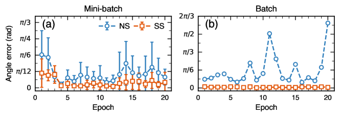
We now evaluate the advantages of the proposed stabilizer-based method of Section II.3.2, over the neural state-based method of Eq. 10, for Monte Carlo estimation of the overlap, which is used to compute the training gradient. For benchmarking purposes, we analyze the errors in the gradient estimates relative to the true gradient, obtained through an exhaustive evaluation of the inner product of Eq. 9. Specifically, we focus on the error in the gradient direction and distinguish between errors calculated over a mini-batch and a full batch of measurements. Figure 2 illustrates the evolution of these errors as the neural quantum state is trained using the true gradient. Figure 2(a) shows that both estimators struggle most with capturing the correct gradient direction during the early stages of training, where the neural quantum state is likely the most different from the target state. However, after several epochs, as the neural state becomes more similar to the target, the stabilizer-based estimation significantly improves, while the neural state estimation remains relatively high and inconsistent. Throughout the entire training process, the stabilizer-based estimator consistently provides estimates with much lower variance, which is essential for training stability. Additionally, our proposed estimator is consistently more accurate than the neural-based estimator. Being an unbiased estimator, the stochastic error due to mini-batching is expected to be cancelled out when averaged over the mini-batches and thus can be lowered using smaller learning rates, albeit at the cost of slower training dynamics. Figure 2(b) shows whether this expected behaviour holds for the given estimators. There is a clear difference between them: the stabilizer-based estimator functions as an unbiased estimator, reducing gradient errors by averaging over mini-batches. In contrast, the neural state-based estimator exhibits a systematic bias throughout the entire training duration, resulting in an extreme accumulation of errors from the true gradient. To eliminate this finite-sample bias, a significant increase in the samples generated by the neural state would be necessary. Therefore, given a fixed computational resource budget, our benchmarking results demonstrate that the stabilizer-based gradient estimation has a significant advantage over the neural state-based gradient estimation, highlighting its potential for optimization.
III.2 Training Performance on Pure GHZ States
In this section, we focus on the reconstruction of pure GHZ states from Pauli and Clifford measurements as a benchmark for the training enhancements we have proposed. In particular, we use the shadow-based cross-entropy (), the empirical cross-entropy (), and the infidelity () as the loss functions. In addition, we employ the estimators Eqs. (10) and (II.3.2) in evaluating the overlap between the neural network and stabilizer states. The superscripts “NS” (for neural state-based samples) and “SS” (for stabilizer-based samples) appear with the corresponding loss function to distinguish between the two estimators.

We illustrate the trainability and the generalization power of these training methods in Fig. 3 via the optimization progress curves of loss functions evaluated on the training set (upper row) and infidelity with respect to the true states (lower row), over 50 epochs. For Pauli measurements, plotted in Fig. 3(a) and (b), the superiority of cross-entropy-based training over the infidelity-based approach is apparent. The latter struggles to achieve significant progress in approximating the underlying quantum state. Moreover, the benefits of the cross-entropy-based loss function become even more pronounced when considering computational costs. Both loss functions rely on computing the overlap between the neural quantum state and stabilizers (see Eq. 9). For the infidelity loss function, each Pauli measurement leads to a proliferation of stabilizers that grows super-exponentially with the number of qubits (see Eq. 4). In contrast, this prohibitive scaling is entirely absent for both cross-entropy-based loss functions, as each Pauli measurement contributes a single stabilizer. In a previous work [2], we attempted to address the prohibitive scaling of the infidelity-based approach through Monte Carlo sampling of stabilizers from a classical shadow state. However, this strategy led to unstable training. Additionally, we note that stabilizer-based training improves in-training performance across all loss functions (the results for neural-state-based cross-entropy loss functions have been omitted for visual clarity). Moreover, these improvements during training translate to enhanced generalization only for cross-entropy loss functions. In fact, for the cross-entropy loss function, stabilizer-based training proves to be crucial.
We now discuss the Clifford measurements, beginning with the benchmarking performed on the six-qubit GHZ state shown in Fig. 3(c) and (d). Our previous observations regarding the advantages of stabilizer-based sampling generalize to this scenario and, in fact, are applicable to the infidelity loss function as well. Indeed, the loss function leads to an improved generalization with the final infidelity of roughly an order of magnitude compared to the loss function , as shown in Fig. 3(d). Interestingly, this improvement in generalization is achieved despite their corresponding loss functions yielding similar values at the end of training. Further examination of Fig. 3(c) and (d) reveals that our loss function greatly outperforms the previously proposed shadow-based loss function [2] in both the convergence rate and generalization. In addition, a comparison between the loss functions and reveals that our cross-entropy estimator leads to a superior convergence rate and lower infidelity, illustrating the benefits of shadow weights extracted from the classical shadow state (see Eq. (7)). Overall, both loss functions and demonstrate the best convergence rates. The loss functions and exhibit the greatest generalization, approaching an infidelity of , while our estimator shows the greatest stability in reaching states in proximity to the true states. An even more drastic difference in performance is observed for the eight-qubit GHZ state, shown in Fig. 3(e) and (f). In this case, the loss functions , , and struggle to escape local minima. While all of the loss functions result in infidelities that remain stuck at , only the loss function stands out, achieving an infidelity as low as . To summarize, our results indicate that our proposed method provides the best training objective for neural networks trained to approximate an underlying quantum state from limited measurements.
III.3 Applications on Mixed GHZ States
In this section, we describe our application of the methods introduced earlier, namely, the shadow-based cross-entropy loss function with stabilizer-based sampling, to mixed quantum states generated by noisy circuits. Specifically, we consider a circuit that prepares a six-qubit GHZ state beginning from the all-zeroes state . The circuit is composed of a Hadamard gate applied to the first qubit, followed by a series of CNOT gates applied to the consecutive pairs of qubits. For the noise model, we assume two-qubit depolarization noise on the CNOT gates. The depolarizing noise channel is parameterized via a noise strength parameter . Motivated by the experimental relevance of our technique, we consider Pauli measurement datasets, as those are less noisy than Clifford measurements. As the ansatz for the density matrix, we employ the purification ansatz Eq. (2) with a transformer neural network used to parameterize . This approach allows us to impose physical constraints on the ansatz.
III.3.1 Pauli Observables
Although classical shadows based on Pauli measurements have been demonstrated to predict local observables with high accuracy, their predictive accuracy worsens in the case of many-body observables. In this section, we demonstrate the benefits of the neural network approach over classical shadows in predicting Pauli observables. To do so, a set of 5000 random Pauli strings is generated by sampling each single-qubit Pauli operator from a uniform distribution.
The absolute error in predicting Pauli observables from neural networks and classical shadows is shown in Fig. 4(a). As expected, the precision and accuracy of estimates extracted from the classical shadow technique become larger as the Pauli weight increases. This poor performance in predicting high weight observables is alleviated by projecting a classical shadow state to a physical state on the probability simplex (see Appendix B). Despite this adjustment, the neural state ansatz consistently demonstrates superior performance across all noise levels. This observation is further supported when focusing solely on prediction accuracy, as highlighted in Fig. 4(b), where we present the same dataset, now normalized by variance and averaged across all noise levels.

III.3.2 Purity and Trace Distance
Continuing our analysis, we broaden our scope to include assessments of purity and trace distance, shown in Fig. 5(a) and (b), respectively. In contrast to the behaviour observed in the case of Pauli observables, projecting the classical shadow state onto the probability simplex leads to a degradation in purity estimation, as shown in Fig. 5(a). However, both neural quantum states and classical shadow states are able to accurately track theoretically predicted results. The distinguishing feature of the physically constrained neural quantum state lies in its ability to consistently provide physical estimates, whereas the classical shadow state’s estimate falls below zero for the least pure target state we consider. As expected, the observed trends of the trace distance shown in Fig. 5(b) align with the results of the Pauli observables: the simplex projection demonstrates successful improvement over the classical shadow state, while the neural quantum state exhibits the lowest error for all noise levels.

Interestingly, we observe relatively weaker performance of the neural quantum states in the low noise regime, specifically and . We investigate this behaviour further by producing visualizations of density matrices, as exemplified in Fig. 5(c), (d), and (e) for . For such high noise levels, all non-zero components in the theoretical density matrix are substantial. In this case, the neural quantum state can successfully capture the full structure of the theoretical density matrix, whereas the classical shadow state is extremely noisy. However, at lower noise regimes, most of the diagonal elements of the density matrix decrease, and only the corner components remain large. The neural quantum state seems to struggle with capturing signals from very small components, possibly due to the Monte Carlo sampling noise present during training, leading to the relative weakening of its performance. We defer a detailed investigation of this phenomenon and the potential enhancements it could bring to neural quantum state tomography in this regime to future studies.
IV Conclusion
In this paper, we have introduced two new concepts for neural quantum state tomography: (a) the shadow-based cross-entropy loss function; and (b) stabilizer-based importance sampling for the estimation of quantum state overlaps. Our benchmarking using Pauli and Clifford measurements collected from pure GHZ states demonstrates a clear improvement in the trainability and the generalization power of the resulting neural quantum states. In particular, we demonstrate the superiority of these neural quantum states in comparison to the conventional neural quantum states trained using log-likelihood optimization and the recently introduced neural quantum states trained using infidelity loss, both of which rely on neural-state-based importance sampling. These advancements enable a significant reduction in both the classical and quantum resources necessary for neural quantum state tomography.
To highlight the significance of our techniques in experimental applications, we employ a physically constrained neural quantum state to reconstruct mixed quantum states from Pauli measurements. In comparison to the classical shadow state constructed from the same dataset, our neural quantum state is much more successful at predicting high-weight and nonlinear observables of both pure and mixed states.
With these promising results, we expect shadow-based neural quantum state tomography to be an invaluable tool for future experiments on near-term quantum devices. Its potential applications span a wide spectrum, from device characterization to quantum simulations in materials science, chemistry, and strong interactions physics. Moving forward, the next steps in the development and exploration of our method will involve scaling it up to accommodate larger systems and validating its utility to a more diverse set of quantum states, specially those prepared experimentally in the near term. One interesting avenue for future research is the characterization of quantum states prepared using analog quantum simulations, wherein the constraints imposed by limited-control electronics present a challenge for quantum state tomography [7].
Appendix A The Transformer Neural Quantum State and Details of Numerical Experiments
We base our neural quantum states on the transformer architecture from Ref. [bennewitz2021] (for details on its implementation, refer to Section I of the supplementary material of that work). More specifically, a quantum state is represented using the transformer model parameterized by the neural network weights as specified in Eq. 1 or Eq. 2, depending on whether the target quantum state is a pure state or a mixed state, respectively. The details of the transformer’s architecture, hyperparameters, and datasets are presented in Table 1. PyTorch [16] is used for the implementation and training of the transformer. The Stim stabilizer-circuit simulator [17] is used for dataset generation and classical shadow state reconstruction. For training, we use the Adam optimizer [18] for stochastic-gradient descent. A cosine annealing schedule is applied to systematically adjust the learning rate throughout training epochs [19]. Finally, early stopping is used to prevent over-fitting.
| Fig. 3 | Figs. 4 and 5 | ||
| Layers | 2 | 2 | |
| Internal dimensions | 8 | 8 | |
| Neural quantum state | Heads | 4 | 4 |
| Trainable parameters | 858 | 954 | |
| Ansatz | Eq. 1 | Eq. 2 with 6 ancilla qubits | |
| Epochs | 50 | 100 | |
| Hyperparameters | Initial learning rate | 0.01 | 0.01 |
| Mini-batch size | 100 | 20 | |
| Monte Carlo samples | 500 | 500 | |
| Dataset | Training | 1000 classical shadows | 3750 classical shadows |
| Validation | – | 1250 classical shadows |
Appendix B Probability Simplex Projection
Unlike the density matrix of a physical quantum state, the classical shadow state is not necessarily positive semidefinite. One approach for obtaining a physical quantum state from a classical shadow state is through a projection onto the probability simplex. Formally, the eigenvalues of the classical shadow state are projected onto the probability simplex , while the eigenvectors are left unchanged. The projected eigenvalues, , are obtained via a minimization of the Euclidean distance:
where denotes the Euclidean norm. We use the algorithm presented in Ref. [20] to perform this minimization.
Acknowledgements
We thank our editor, Marko Bucyk, for his careful review and editing of the manuscript. The authors acknowledge Bill Coish and Christine Muschik for useful discussions. W. K. acknowledges the support of Mitacs and a scholarship through the Perimeter Scholars International program. P. R. acknowledges the financial support of Mike and Ophelia Lazaridis, Innovation, Science and Economic Development Canada (ISED), and the Perimeter Institute for Theoretical Physics. Research at the Perimeter Institute is supported in part by the Government of Canada through ISED and by the Province of Ontario through the Ministry of Colleges and Universities.
References
- Huang et al. [2020] H.-Y. Huang, R. Kueng, and J. Preskill, Predicting many properties of a quantum system from very few measurements, Nat. Phys. 16, 1050–1057 (2020).
- Wei et al. [2023] V. Wei, W. A. Coish, P. Ronagh, and C. A. Muschik, Neural-Shadow Quantum State Tomography, arXiv preprint arXiv:2305.01078 (2023).
- Bennewitz et al. [2021] E. R. Bennewitz, F. Hopfmueller, B. Kulchytskyy, J. Carrasquilla, and P. Ronagh, Neural Error Mitigation of Near-Term Quantum Simulations, Nat. Mach. Intell. 4, 618–624 (2021).
- Ippoliti et al. [2023] M. Ippoliti, Y. Li, T. Rakovszky, and V. Khemani, Operator Relaxation and the Optimal Depth of Classical Shadows, Phys. Rev. Lett. 130, 230403 (2023).
- Rozon et al. [2023] P.-G. Rozon, N. Bao, and K. Agarwal, Optimal twirling depths for shadow tomography in the presence of noise, arXiv preprint arXiv:2311.10137 (2023).
- Hu et al. [2024] H.-Y. Hu, A. Gu, S. Majumder, H. Ren, Y. Zhang, D. S. Wang, Y.-Z. You, Z. Minev, S. F. Yelin, and A. Seif, Demonstration of Robust and Efficient Quantum Property Learning with Shallow Shadows, arXiv preprint arXiv:2402.17911 (2024).
- Hu and You [2022] H.-Y. Hu and Y.-Z. You, Hamiltonian-driven shadow tomography of quantum states, Phys. Rev. Research 4, 013054 (2022).
- Cha et al. [2022] P. Cha, P. Ginsparg, F. Wu, J. Carrasquilla, P. L. McMahon, and E.-A. Kim, Attention-based quantum tomography, Mach. Learn.: Sci. Technol. 3, 01LT01 (2022).
- Hu et al. [2023] H.-Y. Hu, S. Choi, and Y.-Z. You, Classical shadow tomography with locally scrambled quantum dynamics, Phys. Rev. Research 5, 023027 (2023).
- Torlai and Melko [2018] G. Torlai and R. G. Melko, Latent Space Purification via Neural Density Operators, Phys. Rev. Lett. 120, 240503 (2018).
- Hastings et al. [2010] M. B. Hastings, I. González, A. B. Kallin, and R. G. Melko, Measuring Renyi Entanglement Entropy in Quantum Monte Carlo Simulations, Phys. Rev. Lett. 104, 157201 (2010).
- Kulchytskyy [2019] B. Kulchytskyy, Probing universality with entanglement entropy via quantum Monte Carlo, Ph.D. thesis, University of Waterloo (2019).
- Beach et al. [2019] M. J. S. Beach, I. D. Vlugt, A. Golubeva, P. Huembeli, B. Kulchytskyy, X. Luo, R. G. Melko, E. Merali, and G. Torlai, QuCumber: wavefunction reconstruction with neural networks, SciPost Phys. 7, 009 (2019).
- Liu et al. [2023] Z. Liu, Z. Hao, and H.-Y. Hu, Predicting Arbitrary State Properties from Single Hamiltonian Quench Dynamics, arXiv preprint arXiv:2311.00695 (2023).
- Aaronson and Gottesman [2004] S. Aaronson and D. Gottesman, Improved simulation of stabilizer circuits, Physical Review A—Atomic, Molecular, and Optical Physics 70, 052328 (2004).
- Paszke et al. [2019] A. Paszke, S. Gross, F. Massa, A. Lerer, J. Bradbury, G. Chanan, T. Killeen, Z. Lin, N. Gimelshein, L. Antiga, A. Desmaison, A. Köpf, E. Yang, Z. DeVito, M. Raison, A. Tejani, S. Chilamkurthy, B. Steiner, L. Fang, J. Bai, and S. Chintala, PyTorch: An Imperative Style, High-Performance Deep Learning Library, arXiv preprint arXiv:1912.01703 (2019).
- Gidney [2021] C. Gidney, Stim: a fast stabilizer circuit simulator, Quantum 5, 497 (2021).
- Kingma and Ba [2014] D. P. Kingma and J. Ba, Adam: A Method for Stochastic Optimization, arXiv preprint arXiv:1412.6980 (2014).
- Loshchilov and Hutter [2016] I. Loshchilov and F. Hutter, SGDR: Stochastic Gradient Descent with Warm Restarts, arXiv preprint arXiv:1608.03983 (2016).
- Chen and Ye [2011] Y. Chen and X. Ye, Projection Onto A Simplex, arXiv preprint arXiv:1101.6081 (2011).