Boosting of Implicit Neural Representation-based Image Denoiser
Abstract
Implicit Neural Representation (INR) has emerged as an effective method for unsupervised image denoising. However, INR models are typically overparameterized; consequently, these models are prone to overfitting during learning, resulting in suboptimal results, even noisy ones. To tackle this problem, we propose a general recipe for regularizing INR models in image denoising. In detail, we propose to iteratively substitute the supervision signal with the mean value derived from both the prediction and supervision signal during the learning process. We theoretically prove that such a simple iterative substitute can gradually enhance the signal-to-noise ratio of the supervision signal, thereby benefiting INR models during the learning process. Our experimental results demonstrate that INR models can be effectively regularized by the proposed approach, relieving overfitting and boosting image denoising performance.
Index Terms— Image denoising, implicit neural representation, regularization, boosting algorithm
1 Introduction
Image denoising is a fundamental inverse problem in low-level computer vision. In this setting, we are given a vectorized noisy observation combined by the underlying clean signal and noise, which is generally formulated as follows:
| (1) |
where is an additive noise and typically assumed to be i.i.d. zero-mean Gaussian noise, i.e., , where denotes the standard deviation. Extensive algorithms and models have been developed for image denoising. Before the era of deep learning, filter-based methods [1, 2, 3], thresholding methods [4, 5, 6] and block-matching-based methods [7, 8] are representative works. Nowadays, deep neural networks, such as DnCNN [9], SwinIR [10] and Restormer [11], etc., achieve remarkable results. In addition to these supervised learning models, self-supervised methods, such as Noise2Self [12], Noise2Void [13] and Self2Self [14], etc., provide another alternative to improve the signal-to-noise ratio (SNR), which only utilizes a single noisy image during training.
Recent advancements in image denoising have underscored the potential of Implicit Neural Representations (INR). Noteworthy methods include DIP [15], SIREN [16] and WIRE [17], among others. INR offers a novel approach to representing implicitly defined, continuous, and differentiable signals parameterized by neural networks [16]. Through INR, networks are trained to map specific coordinates or even random noise directly to the target denoised representation, efficiently adapting to fit the noisy observation.
However, INR models are typically overparameterized [18]. Consequently, these models are prone to overfitting during training, resulting in suboptimal results, even fitting noisy ones. Existing solutions to this problem primarily pursue the following directions. The first attempts to stop the training once the model begins to fit noise. Early Stopping [18] exemplifies this approach, which utilizes the running variance of past denoised results as a metric to determine the optimal training stopping point. Nevertheless, its performance can be inconsistent, and the hyper-parameter optimization becomes particularly intense. The second one integrates regularization to relieve the overfitting problem, such as Total-Variation (TV) [19], Regularization by Denoising (RED) [20], etc. For example, DIP can be effectively regularized by TV [21, 22], as well as RED [23], namely DeepRED. Although effective, these methods require additional computation and involve further hyperparameter tuning. Furthermore, the boosting algorithm [24, 25, 26, 27] presents a holistic strategy for enhancing the denoised outputs. Yet, despite its generality and efficacy, such methods are typically employed as post-processing measures. This divides the process into two distinct phases: primary denoising followed by the boosting stage. This bifurcation naturally demands additional computations and introduces more hyper-parameters to the process.
In this work, we propose a simple yet effective method to relieve the overfitting tendencies of INR models, thereby boosting their performance. Specifically, our method revolves around iteratively updating the supervision signal with the mean value derived from both the prediction and the original supervision signal throughout the training phase. This iterative substitution approach termed ITS, is shown to enhance the supervision signal’s SNR incrementally. As a result, the learning trajectory of INR models becomes more robust. Unlike conventional techniques, our approach introduces nearly zero extra computational overhead and seamlessly integrates into the learning process of INR models. Our experimental results confirm that the proposed method is an effective regularization tool for INR models, addressing overfitting challenges and boosting overall performance. Our contributions are summarized as follows:
-
•
We propose a general paradigm for regularizing INR models in image denoising to boost their performance.
-
•
We theoretically prove the proposed ITS approach can progressively improve the supervision signal’s SNR.
-
•
We evaluate the proposed method when integrated with typical INR models for image denoising, and experimental results demonstrate the effectiveness of our method.
2 Preliminary
The INR is trained to map from a given coordinate or random noise to the desired denoised representation during the learning process. This can be mathematically formulated as follows:
| (2) |
where denotes the INR model with representing its parameters. The term is the given coordinate [16, 17] or random noise [15].
The overall objective function for optimizing is formulated as follows:
| (3) |
where denotes the norm, and is the regularization term for introducing explicit priors, such as TV [19, 21], RED [20, 23], and others.
For simplicity, let’s consider when , i.e., without any explicit priors, the objective function simplifies to . Within this context, the INR models align with the dominant semantic context (represented by low-frequency signals) before they start overfitting to the noise, symbolized by high-frequency signals [28].
Additionally, when the noise levels increase, the learning becomes more challenging, and INR models are more vulnerable to noise disturbances [18, 29]. In contrast, if the noise level is small, the learning is much easier; more aggressively, in an extreme case that if , the objective function leads to fitting the clean ground truth.
These observations raise a simple question: Can we clean up the noisy supervision signal during the INR training process? If so, the INR model can learn much better because the noise level is reduced to provide a better supervision signal; even more extreme, if we clean up the original noisy supervision signal to the clean ground truth, then the issue of overfitting to noise will be eliminated.
| Baseline | INR | INR w/ ITS (Ours) | ||||||||
|---|---|---|---|---|---|---|---|---|---|---|
| Dataset | BM3D | DnCNN | Restormer | DIP | SIREN | WIRE | DIP | SIREN | WIRE | |
| Set9 | 25 | 30.15 / 0.80 | 30.82 / 0.84 | 32.28 / 0.86 | 28.66 / 0.75 | 28.00 / 0.72 | 27.34 / 0.68 | 28.92(+0.26) / 0.76(+0.01) | 28.24(+0.24) / 0.73(+0.01) | 27.69(+0.35) / 0.70(+0.02) |
| 50 | 26.60 / 0.70 | 27.41 / 0.76 | 28.07 / 0.77 | 22.63 / 0.46 | 23.23 / 0.51 | 23.66 / 0.54 | / | 25.15(+1.92) / 0.62(+0.11) | 24.82(+1.16) / 0.60(+0.06) | |
| 75 | 23.69 / 0.63 | 24.22 / 0.67 | 24.78 / 0.70 | 18.43 / 0.27 | 18.52 / 0.28 | 21.33 / 0.46 | / | / | 22.57(+1.24) / 0.55(+0.09) | |
| 100 | 21.35 / 0.58 | 20.82 / 0.48 | 22.32 / 0.65 | 15.66 / 0.17 | 15.31 / 0.16 | 19.62 / 0.42 | / | / | 20.68(+1.06) / 0.52(+0.10) | |
| Set11 | 25 | 29.94 / 0.84 | 29.98 / 0.85 | 27.88 / 0.72 | 25.93 / 0.67 | 25.65 / 0.65 | 26.09 / 0.67 | 27.10(+1.17) / 0.75(+0.08) | 27.11(+1.46) / 0.72(+0.07) | 26.38(+0.29) / 0.70(+0.03) |
| 50 | 26.16 / 0.74 | 25.93 / 0.73 | 20.97 / 0.44 | 19.68 / 0.38 | 18.34 / 0.35 | 22.11 / 0.50 | / | / | 23.39(+1.28) / 0.56(+0.06) | |
| 75 | 23.49 / 0.65 | 20.51 / 0.42 | 17.44 / 0.30 | 15.71 / 0.23 | 14.02 / 0.19 | 18.96 / 0.37 | / | / | 20.80(+1.84) / 0.46(+0.09) | |
| 100 | 21.43 / 0.58 | 15.16 / 0.20 | 15.69 / 0.23 | 13.16 / 0.15 | 11.49 / 0.12 | 16.81 / 0.29 | / | / | 18.79(+1.98) / 0.38(+0.09) | |


3 Proposed Algorithm
Considering that the INR model is generally optimized using stochastic gradient descent (SGD) within iterations, then for a given -th iteration, the denoised result can be expressed as follows [24, 25, 26, 30]:
| (4) | ||||
where denotes reconstruction error. This error can be further decomposed into two parts: denotes the residual noise from and stands for the lost components of .
Assuming that at iteration, the model begins to overfit the noise, then there exists a relationship between at different iterations, that satisfies:
| (5) |
where , and the above relationship’s shape mimics a bell curve. In a practical setting, it is infeasible to determine since only the noisy observation is available without the information of ground truth .
However, given that the noisy observation is described by Eq.(1), we suggest merging the internal denoised result with noisy observation to generate a renewed supervision signal for -th iteration:
| (6) | ||||
where is a new reconstruction error. If holds true, the above substitution can yield a supervision signal with an enhanced SNR. An illustrative proof is provided in Theorem 1.
Theorem 1.
Proof.
For any iteration (), that model already (imperfectly/partially) fits visual contents yet does not fully fit the noise, we have:
| (7) | ||||
| (8) |
Let , Eq.(8) implies . Considering the SNR of substitution from Eq.(6), we have:
| (9) | ||||
where Eq.(9) follows the Cauchy-Shwartz inequality. Therefore, we have:
| (10) | ||||
| (11) |
Recall that , then we have: . Therefore, the substitution can improve the SNR of the supervision signal. ∎
Remark.
The worse-case of substitution from Eq.(6) is when , i.e., model perfect fits noisy observation, then . And the best case is when , i.e., , which is almost impossible, and no longer need for the substitution.
Based on this observation, we propose an iterative substitution (ITS) strategy that performs the updating from Eq.(6) with given increasing iterations. For simplicity, we introduce a hyperparameter to generate a set of iterations , then for each iteration in , we perform the substitution from Eq.(6), that is:
| (12) |
Corollary 1.1.
For a given set of iterations , assuming , we have , i.e., the SNR of renewed supervision signal in the given set of iterations increases one by one.
The ITS approach capitalizes on the iterative refinement principle during the training process. By progressively substituting the denoised results into the supervision signal, the model constantly refines its understanding of the image and prevents overfitting, thereby enhancing the denoising performance. The increasing iterations ensure that the model doesn’t hastily converge but instead gradually refines its output, potentially achieving a balance between noise suppression and preservation of crucial image details.
4 Experiments
4.1 Experimental Setup
Datasets. We choose two benchmark datasets: Set9 and Set11 [7] for experiments. In detail, Set9 consists of nine RGB colorful images, while Set11 comprises eleven grayscale images.
Noises. We select for simulating different noise levels.
Baselines. We choose three baseline methods: BM3D [7], DnCNN [9], Restormer [11] as baselines for comparison.
INR models. We choose three INR models: DIP [15], SIREN [16], WIRE [17] for experiments. Then, we apply our proposed ITS to them to evaluate the effectiveness of our method.
Evaluation method. For quantitative evaluation, we mainly refer to two metrics: Peak signal-to-noise ratio (PSNR) and structural similarity (SSIM). For qualitative evaluation, we visualize some denoised results.
Implementation details. We utilize the official pre-trained models for baselines: DnCNN and Restormer. Meanwhile, we follow the official implementations for BM3D and INR models: DIP, SIREN, and WIRE.
4.2 Experimental Results
Quantitative results. Table 1 reports experimental results of average PSNR and SSIM for Set9 and Set11 datasets. Restormer consistently presents the best baseline results of all noise levels in Set9, as the underlined values indicate. DnCNN achieves the best performance when in Set11, while BM3D achieves the best results when in Set11. It is worth mentioning that Restormer and DnCNN are pre-trained with large-scale datasets in a supervised manner. Notably, INR models with ITS demonstrate substantial improvement over the standard INR models across various noise levels, as highlighted by boldface. Specifically, with a high noise level, applying ITS in DIP and SIREN results in a great performance enhancement; for example, when on Set9, the PSNR of SIREN increases by 4.06. The enhancements are further validated by paired t-test statistical significance annotations, offering a more generalized perspective on the efficacy of the proposed ITS.
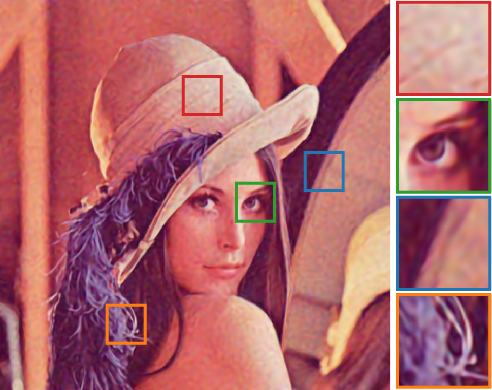
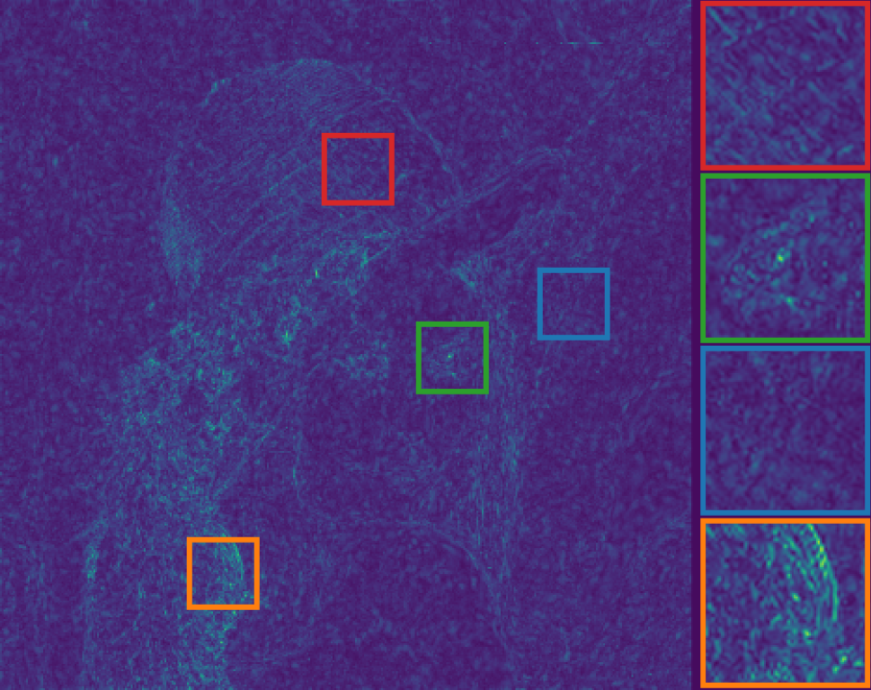
Qualitative results. Fig. 2 visualizes the denoised results from different baselines, as well as INR models and INR models with ITS. To supplement this visual comparison, we further calculate the reconstruction error map from Eq.(4) for each denoised result. According to Eq.(4), such an error map consists of residual noise and lost components; therefore, we utilize robust wavelet-based estimator [31] to estimate the (Gaussian) noise standard deviation on it, to reveal the noise level of residual noise. In detail, we observe that Restormer achieves the best denoised result among baselines. Among the INR models, SIREN delivers a better denoising capability. After introducing ITS, all INR models can be effectively regularized, thereby producing better results with increased PSNR and SSIM. In addition, comparing the reconstruction error map from INR models and those from them applied with ITS, we observe that the error maps for INR models incorporating ITS show a notable reduction in residual noise, as highlighted by the visual content difference and reduced .
4.3 Ablation Study
In this section, we conduct a series of ablation studies to evaluate the effectiveness of our proposed approach.
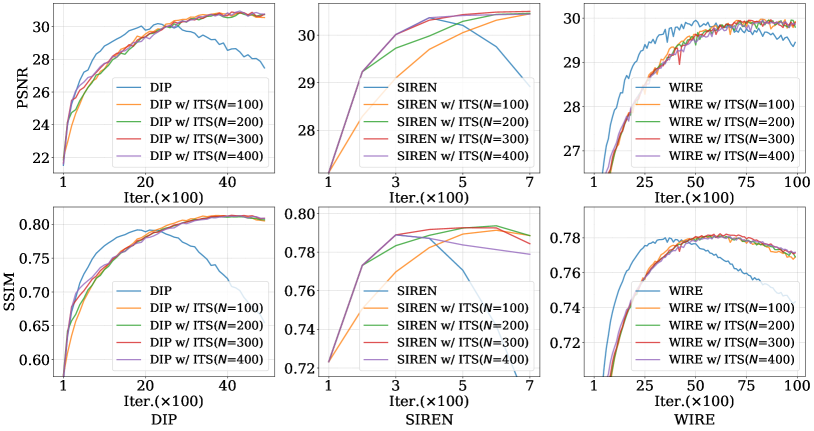
Impact of hyper-parameter: . We study the impact of hyper-parameter on three INR models with Lena. Specifically, we fix and select . The results are presented in Fig. 3. In general, we observe that ITS can boost the performance of three INR models. Besides, we observe that almost all INR models w/ ITS are not sensitive to the hyper-parameter, except the SIREN. In detail, for SIREN w/ ITS, the PSNRs from different hyper-parameters are close in final iterations, while the SSIMs have a gap of around 0.01.
Relieve the overfitting. As illustrated in Table 1 and Fig. 3, the experimental results demonstrate that our method can relieve the overfitting problem of the INR models. The key reason has already been illustrated in Sec. 3, where the proposed ITS can iteratively improve the SNR of the supervision signal.
| Method | Last | Best | Num of Extra | Time (min) |
| PSNR / SSIM | PSNR / SSIM | Hparam. | ||
| Comparison to regularization methods | ||||
| DIP | 26.74 / 0.60 | 30.18 / 0.79 | 0 | 3.33 |
| DIP + WTV | 27.55 / 0.74 | 30.29 / 0.80 | 3 | 135.43 |
| DeepRED | 27.84 / 0.75 | 30.40 / 0.80 | 5 | 26.29 |
| DIP + ITS | 30.31 / 0.79 | 30.95 / 0.81 | 1 | 3.41 |
| Integration to regularization methods | ||||
| DIP + WTV + ITS | 29.98 / 0.78 | 30.40 / 0.80 | 3+1 | 137.45 |
| DeepRED + ITS | 30.13 / 0.79 | 30.87 / 0.81 | 5+1 | 27.50 |
Comparison to regularization methods. We also compare our proposed ITS to regularization methods, including TV and RED. For a fair comparison, we choose the DIP as the baseline model and follow the training configurations from DeepRED [23]. In detail, we follow DeepRED [23] for combining DIP with RED. As for DIP with TV, we utilize a weighted version of TV (WTV) [22], which has been proven to be better compared to ordinary TV [21]. We conduct all experiments on the Lena with . The experimental results are reported in Table 2. It is worth reminding that the best performance is impossible to obtain for real-world denoising, because we do not have the ground truth. We report these best performances only to compare the improvement from different methods and to illustrate the overfitting problem. As shown in Table 2, the proposed ITS outperforms two regularizations according to PSNR and SSIM from the last. In addition, from the performance gap between the last and best, we observe that the proposed ITS can consistently benefit the INR model and lead to less overfitting results, which follows our theoretical justification in Sec. 3.
Integration to regularization methods. We also study integrating ITS into existing regularization methods. For simplicity, we fix the hyper-parameters of the regularization method and integrate ITS into it. As shown in the last two rows of Table 2, we show that integrating ITS into existing regularization methods also brings better results.
Time consumption. As shown in the last column of Table 2, we demonstrate that ITS only brings limited extra time consumption because ITS seamlessly integrates into the learning process of INR by only substituting the supervision signals with improved SNR ones.
5 Conclusion
This work proposes a general iterative substitution (ITS) paradigm for regularizing INR models in image denoising. Our theoretical justification proves that ITS can improve the SNR of the supervision signal, thereby benefiting the learning process of INR models. Our experimental results demonstrate the effectiveness and efficiency of the proposed ITS. The major limitation of our method is that we assume the denoised result contains additive reconstruction error as illustrated in Eq.(4). Although such an assumption is widely adopted in prior works [24, 25, 26, 30], the general assumption for the inverse problem, i.e., , would be more appropriate, which additionally considers transformation formalized by , such as blurring. One future direction is to address the above limitation. In addition, extending our method to video denoising is one future direction. Besides, generalizing our problem and method to the general image inverse problem is another future direction.
6 REFERENCES
References
- [1] Ming Zhang and Bahadir K Gunturk, “Multiresolution bilateral filtering for image denoising,” IEEE Transactions on Image Processing, vol. 17, no. 12, pp. 2324–2333, 2008.
- [2] Antoni Buades, Bartomeu Coll, and Jean-Michel Morel, “A review of image denoising algorithms, with a new one,” Multiscale Modeling & Simulation, vol. 4, no. 2, pp. 490–530, 2005.
- [3] Claude Knaus and Matthias Zwicker, “Dual-domain filtering,” SIAM Journal on Imaging Sciences, vol. 8, no. 3, pp. 1396–1420, 2015.
- [4] S Grace Chang, Bin Yu, and Martin Vetterli, “Adaptive wavelet thresholding for image denoising and compression,” IEEE Transactions on Image Processing, vol. 9, no. 9, pp. 1532–1546, 2000.
- [5] Thierry Blu and Florian Luisier, “The SURE-LET approach to image denoising,” IEEE Transactions on Image Processing, vol. 16, no. 11, pp. 2778–2786, 2007.
- [6] Emmanuel J Candes, Carlos A Sing-Long, and Joshua D Trzasko, “Unbiased risk estimates for singular value thresholding and spectral estimators,” IEEE Transactions on Signal Processing, vol. 61, no. 19, pp. 4643–4657, 2013.
- [7] Kostadin Dabov, Alessandro Foi, Vladimir Katkovnik, and Karen Egiazarian, “Image denoising by sparse 3-d transform-domain collaborative filtering,” IEEE Transactions on Image Processing, vol. 16, no. 8, pp. 2080–2095, 2007.
- [8] Matteo Maggioni, Vladimir Katkovnik, Karen Egiazarian, and Alessandro Foi, “Nonlocal transform-domain filter for volumetric data denoising and reconstruction,” IEEE Transactions on Image Processing, vol. 22, no. 1, pp. 119–133, 2013.
- [9] Kai Zhang, Wangmeng Zuo, Yunjin Chen, Deyu Meng, and Lei Zhang, “Beyond a Gaussian denoiser: Residual learning of deep CNN for image denoising,” IEEE Transactions on Image Processing, vol. 26, no. 7, pp. 3142–3155, 2017.
- [10] Jingyun Liang, Jiezhang Cao, Guolei Sun, Kai Zhang, Luc Van Gool, and Radu Timofte, “SwinIR: Image restoration using swin transformer,” in ICCV Workshops, 2021, pp. 1833–1844.
- [11] Syed Waqas Zamir, Aditya Arora, Salman Khan, Munawar Hayat, Fahad Shahbaz Khan, and Ming-Hsuan Yang, “Restormer: Efficient transformer for high-resolution image restoration,” in CVPR, 2022, pp. 5718–5729.
- [12] Joshua Batson and Loïc Royer, “Noise2Self: Blind denoising by self-supervision,” in ICML, 2019, vol. 97, pp. 524–533.
- [13] Alexander Krull, Tim-Oliver Buchholz, and Florian Jug, “Noise2Void - learning denoising from single noisy images,” in CVPR, 2019, pp. 2129–2137.
- [14] Yuhui Quan, Mingqin Chen, Tongyao Pang, and Hui Ji, “Self2Self with dropout: Learning self-supervised denoising from single image,” in CVPR, 2020, pp. 1887–1895.
- [15] Dmitry Ulyanov, Andrea Vedaldi, and Victor S. Lempitsky, “Deep image prior,” in CVPR, 2018, pp. 9446–9454.
- [16] Vincent Sitzmann, Julien N. P. Martel, Alexander W. Bergman, David B. Lindell, and Gordon Wetzstein, “Implicit neural representations with periodic activation functions,” in NeurIPS, 2020, pp. 7462–7473.
- [17] Vishwanath Saragadam, Daniel LeJeune, Jasper Tan, Guha Balakrishnan, Ashok Veeraraghavan, and Richard G Baraniuk, “WIRE: Wavelet implicit neural representations,” in CVPR, 2023, pp. 18507–18516.
- [18] Hengkang Wang, Taihui Li, Zhong Zhuang, Tiancong Chen, Hengyue Liang, and Ju Sun, “Early stopping for deep image prior,” Transactions on Machine Learning Research, 2023.
- [19] “Nonlinear total variation based noise removal algorithms,” Physica D: Nonlinear Phenomena, vol. 60, no. 1, pp. 259–268, 1992.
- [20] Yaniv Romano, Michael Elad, and Peyman Milanfar, “The little engine that could: Regularization by denoising (RED),” SIAM Journal on Imaging Sciences, vol. 10, no. 4, pp. 1804–1844, 2017.
- [21] Jiaming Liu, Yu Sun, Xiaojian Xu, and Ulugbek S. Kamilov, “Image restoration using total variation regularized deep image prior,” in ICASSP, 2019, pp. 7715–7719.
- [22] Pasquale Cascarano, Andrea Sebastiani, Maria Colomba Comes, Giorgia Franchini, and Federica Porta, “Combining weighted total variation and deep image prior for natural and medical image restoration via ADMM,” in ICCSA, 2021.
- [23] Gary Mataev, Peyman Milanfar, and Michael Elad, “DeepRED: Deep image prior powered by red,” in ICCV Workshops, 2019.
- [24] Yaniv Romano and Michael Elad, “Boosting of image denoising algorithms,” SIAM Journal on Imaging Sciences, vol. 8, no. 2, pp. 1187–1219, 2015.
- [25] Chang Chen, Zhiwei Xiong, Xinmei Tian, and Feng Wu, “Deep boosting for image denoising,” in ECCV, 2018, pp. 3–19.
- [26] Chang Chen, Zhiwei Xiong, Xinmei Tian, Zheng-Jun Zha, and Feng Wu, “Real-world image denoising with deep boosting,” IEEE Transactions on Pattern Analysis and Machine, vol. 42, no. 12, pp. 3071–3087, 2020.
- [27] Jiayi Ma, Chengli Peng, Xin Tian, and Junjun Jiang, “DBDnet: A deep boosting strategy for image denoising,” IEEE Transactions on Multimedia, vol. 24, pp. 3157–3168, 2022.
- [28] Zhi-Qin John Xu, Yaoyu Zhang, Tao Luo, Yanyang Xiao, and Zheng Ma, “Frequency principle: Fourier analysis sheds light on deep neural networks,” Communications in Computational Physics, vol. 28, no. 5, pp. 1746–1767, 2020.
- [29] Wentian Xu and Jianbo Jiao, “Revisiting implicit neural representations in low-level vision,” in ICLR Workshops, 2023.
- [30] Geonwoon Jang, Wooseok Lee, Sanghyun Son, and Kyoung Mu Lee, “C2N: Practical generative noise modeling for real-world denoising,” in ICCV, 2021, pp. 2330–2339.
- [31] David L Donoho and Iain M Johnstone, “Ideal spatial adaptation by wavelet shrinkage,” Biometrika, vol. 81, no. 3, pp. 425–455, 1994.