form factors from lattice QCD
Abstract
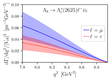
We present the first lattice-QCD determination of the form factors describing the semileptonic decays and , where the and are the lightest charm baryons with and , respectively. These decay modes provide new opportunities to test lepton flavor universality and also play an important role in global analyses of the strong interactions in semileptonic decays. We determine the full set of vector, axial vector, and tensor form factors for both decays, but only in a small kinematic region near the zero-recoil point. The lattice calculation uses three different ensembles of gauge-field configurations with flavors of domain-wall fermions, and we perform extrapolations of the form factors to the continuum limit and physical pion mass. We present Standard-Model predictions for the differential decay rates and angular observables. In the kinematic region considered, the differential decay rate for the final state is found to be approximately 2.5 times larger than the rate for the final state. We also test the compatibility of our form-factor results with zero-recoil sum rules.
I Introduction
Semileptonic decays are used to determine the CKM matrix element and to search for deviations from lepton flavor universality Gambino:2020jvv ; Bifani:2018zmi ; Bernlochner:2021vlv . They also provide an important testing ground for heavy-quark effective theory Neubert:1993mb . In recent years, the operation of the Large Hadron Collider has provided new opportunities for measurements involving baryons. The simplest baryonic process is , in which both the initial and final hadrons are the ground states with . This mode has been used in combination with to determine Detmold:2015aaa ; Aaij:2015bfa and offers the prospect of measuring the -versus- ratio and related observables Bifani:2018zmi ; Bernlochner:2021vlv . The baryonic decays can provide complementary information on physics beyond the Standard Model when compared with mesonic decays Dutta:2015ueb ; Li:2016pdv ; Albrecht:2017odf ; Datta:2017aue ; Alioli:2017ces ; Ray:2018hrx ; Boer:2019zmp ; Penalva:2019rgt ; Ferrillo:2019owd ; Mu:2019bin ; Hu:2020axt . The form factors have been computed using lattice QCD Bowler:1997ej ; Gottlieb:2003yb ; Detmold:2015aaa ; Datta:2017aue , and the lattice results predict a shape for the differential decay rate in the Standard Model that is consistent with the LHCb measurement Aaij:2017svr . Heavy-quark symmetry provides strong constraints on , in which the light hadronic degrees of freedom have total angular momentum zero. In the heavy-quark-effective-theory (HQET) description of this decay, no subleading order- Isgur-Wise functions occur and only two sub-subleading Isgur-Wise functions enter at order ; the available lattice and LHCb results are well described by a fit of this order Bernlochner:2018kxh ; Bernlochner:2018bfn .
In addition to , the LHCb detector has also collected (and will continue to collect) large numbers of and samples Aaij:2017svr ; the relative branching fractions of these modes have been measured by the CDF Collaboration to be and Aaltonen:2008eu . The and are the lightest charm baryons with and , respectively, and are very narrow resonances decaying to Zyla:2020zbs . It has been projected that can be measured using LHCb data with approximately 17 percent uncertainty at the end of LHC Run 3, and as low as 5 percent uncertainty at the end of Run 6 Bernlochner:2021vlv . To predict in the Standard Model and beyond, the form factors are needed. A calculation of these form factors may also improve the control of the backgrounds in a measurement of . Another potential impact will be on zero-recoil sum rules Mannel:2015osa ; Boer:2018vpx and on global analyses of form factors using dispersion relations Cohen:2019zev . The authors of Ref. Cohen:2019zev wrote “Given the large fractional saturation of the unitarity bounds by , the inclusion of could be particularly fruitful once such data is available.” Finally, we note that there is significant interest in the structure and strong decays of the and , in part due to the closeness of the thresholds Blechman:2003mq ; Guo:2016wpy ; Arifi:2018yhr ; Nieves:2019kdh ; Nieves:2019nol .
In the limit of heavy charm quarks, the light degrees of freedom in and have total angular momentum 1 and these two baryons become degenerate. Note that there is no heavy-quark spin-symmetry relation between the and the due to the different quantum numbers of the light degrees of freedom. This difference also means that the normalization of the leading Isgur-Wise function for remains unconstrained in the heavy-quark limit, and the matrix elements vanish at zero recoil Roberts:1992xm ; Leibovich:1997az . The HQET relations for the and vector and axial vector form factors including the subleading order- contributions were derived in Refs. Roberts:1992xm , Leibovich:1997az , and Boer:2018vpx ; the authors of the latter reference specifically studied the possibility of using HQET fits to LHCb data for the muonic decay to make Standard-Model predictions for . It is still an open question how well HQET at this order can describe these transitions.
Quark-model studies of the and form factors can be found in Refs. Pervin:2005ve ; Gutsche:2017wag ; Gutsche:2018nks ; Becirevic:2020nmb . In the following, we present the first lattice-QCD determination of these form factors. Our calculation follows that of the form factors in Ref. Meinel:2020owd and uses the same ensembles of gauge-field configurations. We observe that the and energy levels for our simulation parameters are below all potential strong-decay thresholds, although they come quite close at the lowest pion mass. As in Ref. Meinel:2020owd , we work in the rest frame of the final-state baryon to avoid mixing between and and between negative and positive parity. This again limits the kinematic coverage to the region near .
Our definitions of the form factors are given in Sec. II. Following a brief summary of the lattice parameters in Sec. III, we discuss the baryon interpolating fields, two-point functions, and the results for the masses in Sec. IV. The extraction of the form factors from three-point functions is described in Sec. V, and their extrapolation to the physical pion mass and continuum limit is discussed in Sec. VI. We test the compatibility with zero-recoil sum rules in Sec. VII and present the Standard-Model predictions for and in Sec. VIII. Our conclusions are given in Sec. IX, and Appendix A contains relations to other form factor definitions used in the literature.
II Definitions of the form factors
In the following, we denote the and as and , respectively. The masses and total decay widths determined by experiments are , , , () Zyla:2020zbs . We neglect the decay widths throughout this work. In our lattice calculations at heavier-than-physical pion masses, the strong decays are in fact kinematically forbidden, except perhaps at the lightest pion mass; the hadron masses we find on the lattice are given in Sec. IV.
We normalize the baryon states as
| (1) | |||||
| (2) | |||||
| (3) |
and work with Dirac and Rarita-Schwinger spinors satisfying
| (4) | |||||
| (5) | |||||
In the equations throughout this paper, Minkowski-space gamma matrices and the metric are used, except where indicated otherwise. We introduce the notation
| (7) | |||||
| (8) |
and
| (9) |
where . We use a helicity basis for all form factors. For the final state, our definition follows the one introduced previously for final states Feldmann:2011xf except for the changes resulting from the opposite parity [note the in Eq. (7)]:
| (10) | |||||
| (11) | |||||
| (12) | |||||
| (13) | |||||
For the final state, we use the definition introduced by us in Ref. Meinel:2020owd , which reads
| (14) | |||||
| (15) | |||||
Only the vector and axial-vector form factors are needed to describe decays in the Standard Model, but we also compute the tensor form factors. Above, . Note that the overall sign of the form factors for each decay mode depends on the phase conventions of the states. This means that also the relative overall sign between the two different final states is left undetermined. Relations between our form-factor definitions and alternative definitions used in the literature are given in Appendix A.
III Lattice actions and parameters
The lattice actions and parameters used in this work are the same as in our calculation of form factors Meinel:2020owd , except that here the valence strange quark is replaced by a valence charm quark. For the latter, we employ the same form of action and analogous tuning conditions as for the bottom quark Aoki:2012xaa , i.e., an anisotropic clover action with bare parameters , , tuned to obtain the correct meson kinetic mass, rest mass, and hyperfine splitting (our notation for the bare parameters follows Ref. Brown:2014ena , while Ref. Aoki:2012xaa uses , , ). The values of these parameters are given in Table 1. The gauge-field ensembles with flavors of domain-wall fermions were generated by the RBC and UKQCD Collaborations Aoki:2010dy ; Blum:2014tka . For the up and down valence quarks, we reuse the domain-wall propagators computed for Ref. Meinel:2020owd . Our computation utilizes all-mode averaging Blum:2012uh ; Shintani:2014vja , in which unbiased estimates with small statistical uncertainties are obtained at reduced cost by combining “exact” and “sloppy” samples.
| Label | [fm] | ||||||||||||
|---|---|---|---|---|---|---|---|---|---|---|---|---|---|
| C01 | 283 | 9056 | |||||||||||
| C005 | 311 | 9952 | |||||||||||
| F004 | 251 | 8032 |
IV Two-point functions and hadron masses
| Up and down quarks | Bottom quarks | Charm quarks | ||||||||||||
|---|---|---|---|---|---|---|---|---|---|---|---|---|---|---|
| Coarse | ||||||||||||||
| Fine | ||||||||||||||
We now move to the discussion of the baryon interpolating fields, two-point functions, and results for the masses. For the , everything is identical to Ref. Meinel:2020owd . The has the same isospin and spin-parity quantum numbers as the (, ), but with a charm quark instead of a strange quark. We therefore use the interpolating field
| (18) |
which differs from Eq. (18) of Ref. Meinel:2020owd only by the replacement . As before, this form will work only at zero momentum. The tilde indicates gauge-covariant Gaussian smearing of the quark fields with the parameters given in Table 2. The field (18) actually has nonzero overlap with both the and the ,
| (19) | |||||
| (20) |
and we can isolate the and components111At zero momentum, the continuum and irreducible representations subduce identically to the and irreducible representations of the double-cover of the cubic group Johnson:1982yq ; the next-higher values of that subduce to the same cubic irreps are and , respectively, and such states will have higher energies. It is therefore safe to refer to only the continuum quantum numbers in this case. using the projectors
| (21) | |||||
| (22) |
The zero-momentum two-point functions are defined like those for the in Ref. Meinel:2020owd , and after applying the above projectors their spectral decomposition reads
| (23) | |||||
| (24) | |||||
At this point the reader may wonder why we did not analyze the with in Ref. Meinel:2020owd , despite being able to project to with the available data. The reason is that we do not trust the single-hadron/narrow-width approximation for the , which has a larger decay width than the and likely a two-pole structure Oller:2000fj .
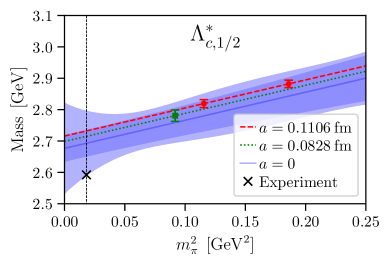
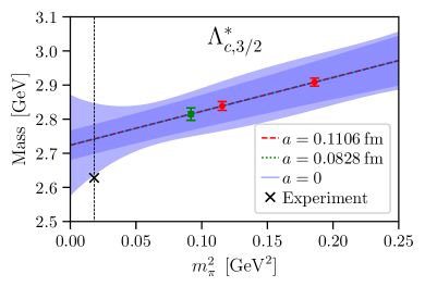
The masses extracted from single-exponential fits to our results for and in the plateau regions are given in Table 3, along with the masses of potential decay products. The latter are not used in our determination of the form factors but are included to assess whether the baryons are stable under the strong interactions for our quark masses. We find that both and are lower than all of the following: , , , although the difference becomes consistent with zero for the F004 ensemble within the statistical uncertainties. The results are of course affected by the finite volume to some degree, but it appears likely that both the and the are stable hadrons at least on the C01 and C005 ensembles, where the energies are well below all thresholds.
We also performed simple chiral-continuum extrapolations of and of the form
| (25) |
with fit parameters , , , and constants , . These fits yield MeV, MeV. To estimate systematic uncertainties associated with the choice of fit model, we additionally performed higher-order fits of the form
| (26) |
with Gaussian priors and , and computed the systematic uncertainties using
| (27) |
where , denote the central value and uncertainty obtained using the parameter values and covariance matrix of the nominal fit and , denote the central value and uncertainty obtained using the parameter values and covariance matrix of the higher-order fit. In this way we finally obtain
| (28) | |||||
| (29) |
which are consistent with the experimental values of , Zyla:2020zbs . Plots of the extrapolations are shown in Fig. 1. Note that we do not use the chiral-continuum extrapolations of the baryon masses in our determination of the form factors; we use the lattice baryon masses when computing the form factors on each ensemble, and then extrapolate only the form factors themselves. The mass extrapolations merely provide a test of our methodology. Finally, in Table 3 we also list the hyperfine splittings computed on each ensemble. Their relative uncertainties are too large to obtain a useful chiral-continuum extrapolation, but the results are consistent within with the experimental value of MeV on each ensemble.
| Label | |||||||||
|---|---|---|---|---|---|---|---|---|---|
| C01 | |||||||||
| C005 | |||||||||
| F004 |
V Three-point functions and form factors
As in Ref. Meinel:2020owd , we compute forward and backward three-point functions
| (30) | |||||
| (31) |
where is the momentum, is the Dirac matrix in the weak current, is the source-sink separation, and is the current-insertion time. With both the and quarks implemented using anisotropic clover actions, the current now includes -improvement terms for both quarks:
| (32) |
Here, are the Euclidean spatial gamma matrices, and are the gauge-covariant symmetric lattice derivatives. The overall matching factors in the current are written as Hashimoto:1999yp ; ElKhadra:2001rv , where are the matching factors for the flavor-conserving temporal vector currents . We determined the values of nonperturbatively using the charge-conservation condition for three-point functions with and meson interpolating fields; the results are given in Table 4. With this choice, the residual matching factors are equal to 1 at tree level and can be computed in perturbation theory without introducing large uncertainties. For the vector and axial-vector currents, we use the one-loop results given in Table III of Ref. Detmold:2015aaa . Here we use more accurately tuned parameters in the - and -quark actions, but we expect the resulting change in the matching factors to be negligible. For the tensor currents, one-loop results are not presently available so we set and estimate the resulting systematic uncertainty at to be 4.04% as in Ref. Datta:2017aue . The values of the -improvement coefficients for all currents are also computed at tree level and are given in Table 4.
| Coarse lattice (C01, C005) | |||||
|---|---|---|---|---|---|
| Fine lattice (F004) |
We generated data for the same two choices of momenta as in Ref. Meinel:2020owd , and , and for slightly larger source-sink separations: at the coarse lattice spacing and at the fine lattice spacing. Here we project the field in the three-point functions to both and , and the spectral decompositions read
| (33) | |||||
| (34) | |||||
where , and , contain the form factors as explained in Sec. II.
In the following, we introduce a label denoting the type of weak current, such that the matrix in Eq. (32) is equal to
| (35) |
We also introduce a label for the different helicities. As in Ref. Meinel:2020owd , we compute the quantities
| (36) |
where are the quantum numbers of the . Here, denotes a constant fit at large to a ratio of three-point and two-point functions that is constructed such that at large it becomes equal to the square of the form factor associated with current and helicity . The quantities are linear projections of the three-point functions proportional to the form factor with current and helicity . In this way, the relative signs of the form factors are preserved, and becomes equal to the form factor of interest at large , which is then extracted from a constant fit. The choice of reference form factor is arbitrary in principle, and we select it based on the signal-to-noise ratio and quality of the ground-state plateau.
The equations for were given in Ref. Meinel:2020owd and we do not repeat them here. For , the construction of is similar to that used previously for in Refs. Detmold:2015aaa ; Detmold:2016pkz . We define
| (37) | |||||
| (38) | |||||
| (39) | |||||
where
| (40) |
for any four-vector , and denotes the three-dimensional unit vector in direction . Above, repeated Greek indices are summed over from 0 to 3, while Latin indices are summed only over the spatial directions. The ratios are equal to kinematic factors depending on the baryon energies times the squares of individual helicity form factors, up to excited-state contamination that decays exponentially for and both large. We then set [or average over and in the case of odd ] and divide out the kinematic factors to obtain
| (41) | |||||
| (42) | |||||
| (43) | |||||
| (44) | |||||
| (45) | |||||
| (46) | |||||
| (47) | |||||
| (48) | |||||
| (49) | |||||
| (50) | |||||
The linear projections of the three-point functions are constructed using
| (51) | ||||
| (52) |
where
| (53) | ||||
| (54) | ||||
| (55) |
with the polarization vectors
| (56) |
To improve the signals, we use the average of the forward three-point function and the Dirac adjoint of the backward three-point function instead of just . We then divide out appropriate kinematic factors to obtain
| (57) | ||||
| (58) | ||||
| (59) | ||||
| (60) | ||||
| (61) | ||||
| (62) | ||||
| (63) | ||||
| (64) | ||||
| (65) |
| (66) | ||||
| (67) | ||||
| (68) | ||||
| (69) | ||||
| (70) | ||||
| (71) | ||||
| (72) | ||||
| (73) | ||||
| (74) |
| (75) | ||||
| (76) | ||||
| (77) | ||||
| (78) | ||||
| (79) | ||||
| (80) |
| (81) | ||||
| (82) | ||||
| (83) | ||||
| (84) | ||||
| (85) | ||||
| (86) |
such that the unwanted factors of cancel in Eq. (36) at large .
For , we use , . Sample results for and our constant fits thereof are shown in Fig. LABEL:fig:ratios12. For , we use , as in Ref. Meinel:2020owd . Sample results for and our constant fits thereof are shown in Fig. LABEL:fig:ratios32. The values of the form factors obtained from the constant fits are listed in Tables 5 and 6. The fits were done individually for each form factor and take into account the correlations between the data at different . The values of range between approximately 0.5 and 1.0, where typically . The correlations between the results for different form factors and different momenta on a given ensemble were evaluated using bootstrap resampling.
| Form factor | C01 | C005 | F004 | |||||
|---|---|---|---|---|---|---|---|---|
| 2 | ||||||||
| 3 | ||||||||
| 2 | ||||||||
| 3 | ||||||||
| 2 | ||||||||
| 3 | ||||||||
| 2 | ||||||||
| 3 | ||||||||
| 2 | ||||||||
| 3 | ||||||||
| 2 | ||||||||
| 3 | ||||||||
| 2 | ||||||||
| 3 | ||||||||
| 2 | ||||||||
| 3 | ||||||||
| 2 | ||||||||
| 3 | ||||||||
| 2 | ||||||||
| 3 |
| Form factor | C01 | C005 | F004 | |||||
|---|---|---|---|---|---|---|---|---|
| 2 | ||||||||
| 3 | ||||||||
| 2 | ||||||||
| 3 | ||||||||
| 2 | ||||||||
| 3 | ||||||||
| 2 | ||||||||
| 3 | ||||||||
| 2 | ||||||||
| 3 | ||||||||
| 2 | ||||||||
| 3 | ||||||||
| 2 | ||||||||
| 3 | ||||||||
| 2 | ||||||||
| 3 | ||||||||
| 2 | ||||||||
| 3 | ||||||||
| 2 | ||||||||
| 3 | ||||||||
| 2 | ||||||||
| 3 | ||||||||
| 2 | ||||||||
| 3 | ||||||||
| 2 | ||||||||
| 3 | ||||||||
| 2 | ||||||||
| 3 |
VI Chiral and continuum extrapolations of the form factors
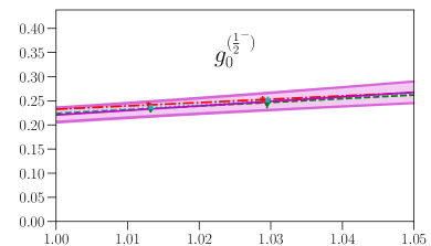
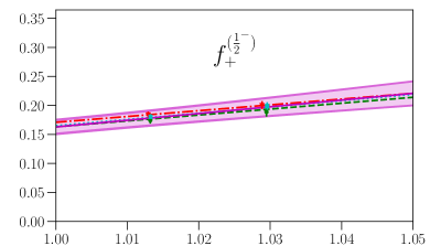
As in Ref. Meinel:2020owd , we extrapolate the lattice results for the form factors to the continuum limit and the physical pion mass using the model
| (87) |
with fit parameters , , , , , for each form factor , and using the kinematic variable
| (88) |
where or depending on the final state considered. In the physical limit , , the functions reduce to
| (89) |
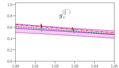
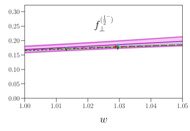
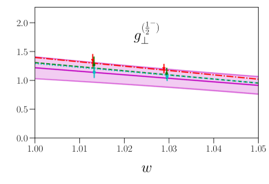
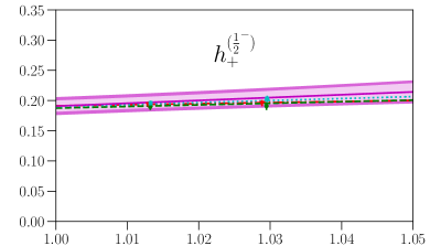
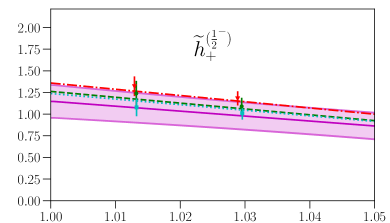
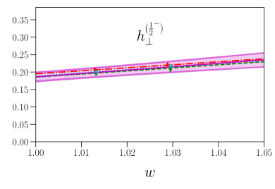
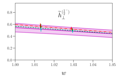
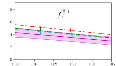
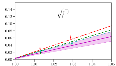
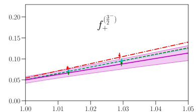
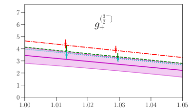
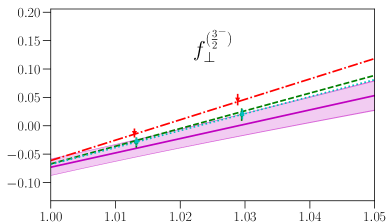
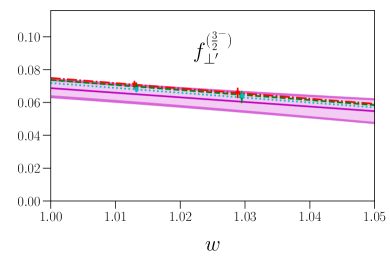
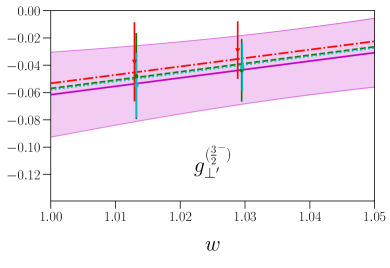
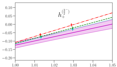
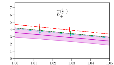
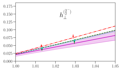
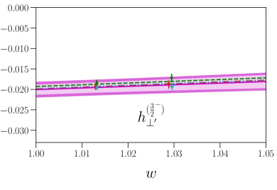
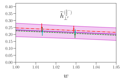
This parametrization corresponds to a Taylor expansion of the shape of the form factors around the endpoint , i.e. an expansion in powers of ; because we have lattice results for only two different kinematic points near and , we work only to first order, and we expect the parametrization to become unreliable for large . Our results for and from fits using Eq. (87) are given in the first two columns of Table 7, and the values and full covariance matrices (evaluated using bootstrap) are also provided as supplemental files. As can be seen in Figs. 4, 5, 6, and 7, the lattice data are well described by the model. The fits of the individual form factors have in the range from approximately 0.5 to 1.5, where we count , , , and as parameters that are primarily constrained by the data, such that .
Again following Ref. Meinel:2020owd , to estimate systematic uncertainties associated with the chiral and continuum extrapolations, we also performed “higher-order” fits including additional terms describing the dependence on the lattice spacing and pion mass,
| (90) | |||||
No priors were used for the parameters , , , . The Gaussian priors for the parameters describing the lattice-spacing and pion-mass dependence were chosen as in Ref. Meinel:2020owd except for and . These coefficients describe the effects of the incomplete improvement of the weak currents in Eq. (32), and here we take the prior widths for and to be two times larger than in Ref. Meinel:2020owd , based on the observation in Ref. Detmold:2015aaa that these effects may be larger for a heavy-to-heavy current than for a heavy-to-light current. These widths allow for missing corrections as large as 10% at the coarse lattice spacing, motivated by the large -quark momenta used here. In the higher-order fits, we also multiplied the data for each form factor with Gaussian random distributions of central value 1 and appropriate widths to incorporate estimates of systematic uncertainties associated with the residual matching factors (2% for the vector and axial vector currents, 4.04% for the tensor currents Datta:2017aue ) and systematic uncertainties associated with neglecting the down-up quark-mass difference and QED corrections [ and ]. Furthermore, to include the scale-setting uncertainty, we also promoted the lattice spacings to fit parameters with Gaussian priors according to the values and uncertainties shown in Table 1. All of our lattice calculations were performed with , and we therefore expect finite-volume effects to be negligible at least for the heavier pion masses where the and are well below strong-decay thresholds. However, we are unable to provide a quantitative estimate of finite-volume effects in the extrapolated form factors.
In the physical limit, the higher-order fits reduce to the same form as in Eq. (89) but with parameters and . Our results for these parameters are given in the last two columns in Table 7 and also in supplemental files. For any observable , we evaluate the form-factor systematic uncertainty using
| (91) |
where , denote the central value and uncertainty calculated using and their covariance matrix, and , denote the central value and uncertainty calculated using and their covariance matrix. We find that the (vector and axial-vector) form-factor systematic uncertainties result in an approximately 12 to 13 percent systematic uncertainty in the differential decay rate in the kinematic range shown in Sec. VIII, and 14 to 18 percent for . Because the decay rates depend quadratically on the form factors, this corresponds to “average” systematic uncertainties of around 6% in the vector and axial-vector form factors and around 8% for .


VII Comparison with zero-recoil sum rules
At zero recoil (), approximate sum-rule bounds on the size of heavy-to-heavy form factors can be derived using the operator product expansion and heavy-quark effective theory Shifman:1994jh ; Bigi:1994ga ; Gambino:2010bp ; Gambino:2012rd ; Mannel:2015osa ; Boer:2018vpx . In Ref. Mannel:2015osa , it was found that the lattice results for the form factors with the final state (which constitute the “elastic” contribution to the sum rule) almost completely saturate the bounds derived through order , apparently leaving very little room for “inelastic” contributions from other final states such as the ’s considered here. However, in the case of -meson decays, the size of and corrections has been found to be approximately 33% of the size of the and terms Gambino:2012rd ; Boer:2018vpx . Allowing for effects of this size also for decays, the authors of Ref. Boer:2018vpx then obtained estimates of the size of the inelastic contributions, which are expected to be dominated by and .
When expressed in terms of our form-factor definitions using the relations given in Appendix A.3, Eqs. (46), (48), (50), and (52) of Ref. Boer:2018vpx become
| (92) | |||||
| (93) | |||||
| (94) | |||||
| (95) |
The zero-recoil sum-rule estimate obtained in Ref. Boer:2018vpx is
| (96) | |||||
| (97) |
Using our lattice-QCD results for the form factors, we find
| (98) | |||||
| (99) |
Thus, our result for the axial current falls within the range given in Ref. Boer:2018vpx , while our result for the vector current is slightly above the upper limit.
VIII observables
The two-fold differential decay rates of and in the Standard Model can be written as
| (100) |
where is the helicity angle of the charged lepton and , , are functions of only Boer:2018vpx . The superscript is used to distinguish the and final states. The equations for , , and in terms of the form factors are given in Ref. Boer:2018vpx (where etc.) and can be converted to our conventions using the relations in Appendix A.3. The integral over yields the -differential decay rate
| (101) |
and we also consider two angular observables Boer:2018vpx : the forward-backward asymmetry
| (102) |
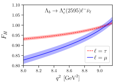
and the “flat term”
| (103) |
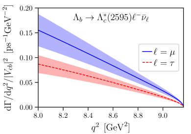
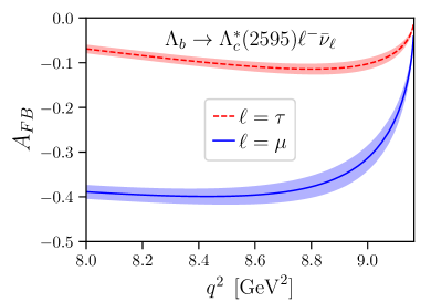
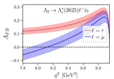
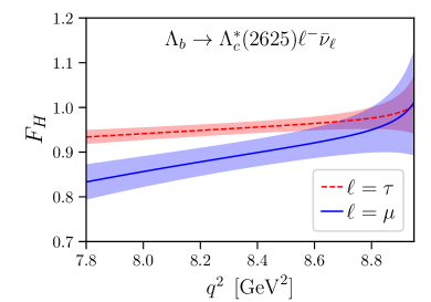
The Standard-Model predictions for and for the angular observables using our form-factor results are shown in Fig. 8. Note that at leading order in heavy-quark effective theory, the differential decay rate for the final state would be a factor 2 smaller than the differential rate for , and the lepton-side angular observables considered here would be equal for both final states Leibovich:1997az ; Boer:2018vpx . In contrast, we find the rate to be approximately 2.5 times larger than the rate, and we find the forward-backward asymmetries to have opposite signs at high . Leading-order HQET is of course expected to be inadequate for these decays, in which the light degrees of freedom in the final state have a different angular momentum than in the initial state. The forms of the subleading corrections are known Leibovich:1997az ; Boer:2018vpx , but we have not been able to obtain an acceptable HQET fit to the full set of form factors even when including these corrections, suggesting that sub-subleading terms may also be significant.
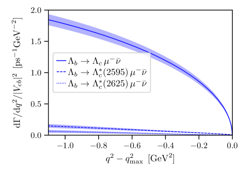
In Fig. 9 we additionally compare the , and differential decay rates with that of , using the form factors from Ref. Detmold:2015aaa for the latter. For example, at , the differential decay rate is approximately 13 times smaller than the differential decay rate. Finally, recall that the CDF Collaboration has measured the total (i.e., integrated over all ) decay rates, and found the total rate to be approximately 1.7 times larger than the total rate Aaltonen:2008eu . Since our results for the differential decay rates at high show the opposite behavior, the differential rates must cross at some value of lower than considered here.
IX Conclusions
The decays and are interesting processes that deserve to be studied in detail, both experimentally and theoretically, to obtain a more complete picture of semileptonic decays. This work contributes to this goal by providing the first lattice-QCD determination of the complete set of form factors, albeit only in the vicinity of . The calculation was made possible by the technology developed initially for Meinel:2020owd : working in the rest frame of the to avoid mixing with unwanted quantum numbers, and using an interpolating field with gauge-covariant spatial derivatives to obtain a good overlap with the .
In nature, the and are narrow resonances decaying through the strong interaction to , with widths of and , respectively Zyla:2020zbs . These values justify the use of the narrow-width approximation. In our lattice calculation with three different pion masses in the range from approximately 300 to 430 MeV, we find that the masses are below all possible strong-decay thresholds, including , except perhaps at the lowest pion mass. Simple chiral-continuum extrapolations of our lattice results for and yield values in agreement with experiment once systematic uncertainties are taken into account. The hyperfine splittings are also found to be consistent with experiment.
We use helicity-based definitions of the and form factors. On each ensemble we performed calculations for two different momenta corresponding to and , where . The final results for the form factors, obtained from extrapolations to the continuum limit and physical pion mass, are parametrized as linear functions of . These parametrizations are expected to be accurate only near the kinematic region where we have lattice data. Our results for the form factors at are compatible (albeit only marginally in the case of the vector form factors) with the zero-recoil sum-rules given in Ref. Boer:2018vpx . It will also be interesting to see the impact on unitarity bounds in global analyses of form factors Cohen:2019zev .
Using our form-factor results, we evaluated the and differential decay rates, forward-backward asymmetry, and flat term in the Standard Model. We find the differential rates to be approximately 2.5 times higher than the differential rates (in the kinematic region considered; the CDF measurement of the total rates Aaltonen:2008eu suggests that the ordering of the differential rates will switch at lower ), which is opposite to the behavior predicted by leading-order HQET but consistent with the expectation that subleading contributions in HQET are important for these types of decays. While not discussed in detail in this paper, we also attempted HQET fits at order Leibovich:1997az ; Boer:2018vpx to our form factor results, but we did not obtain an acceptable description. We expect that corrections, which have not yet been studied for these processes, are also large. This will make it more challenging to combine experimental data for the shapes of the muonic decay rates in the entire kinematic range with the lattice results for the form factors near to obtain Standard-Model predictions for . Lattice calculations at lower , while still working in the rest frame, could be performed using finer lattices or using a moving-NRQCD action Horgan:2009ti for the quark. Alternatively, one could use nonzero momenta and explicitly deal with the mixing of quantum numbers by extracting multiple states using larger operator bases; see for example Refs. Menadue:2013kfi ; Silvi:2021uya .
Acknowledgments
We thank Marzia Bordone and Danny van Dyk for discussions, and the RBC and UKQCD Collaborations for making their gauge field ensembles available. SM is supported by the U.S. Department of Energy, Office of Science, Office of High Energy Physics under Award Number DE-SC0009913. GR is supported by the U.S. Department of Energy, Office of Science, Office of Nuclear Physics, under Contract No. DE-SC0012704 (BNL). The computations for this work were carried out on facilities at the National Energy Research Scientific Computing Center, a DOE Office of Science User Facility supported by the Office of Science of the U.S. Department of Energy under Contract No. DE-AC02-05CH1123, and on facilities of the Extreme Science and Engineering Discovery Environment (XSEDE) XSEDE , which is supported by National Science Foundation grant number ACI-1548562. We acknowledge the use of Chroma Edwards:2004sx ; Chroma , QPhiX JOO2015139 ; QPhiX , QLUA QLUA , MDWF MDWF , and related USQCD software USQCD .
Appendix A Relations between different form factor definitions
In this appendix, we provide expressions for the and form factors in other definitions used in the literature (for the vector and axial-vector currents only) in terms of our form factors. Note that the overall sign of the form factors for each decay mode depends on the phase conventions of the states. Thus, in the following relations, only the relative signs among the form factors for a specific final state are well-determined. To make this explicit, we introduce factors of below, which can take on the values .
A.1 Definition used by Leibovich and Stewart as well as Pervin, Roberts, and Capstick
We find that the form factor definitions in Ref. Leibovich:1997az are related to ours as
| (104) | |||||
| (105) | |||||
| (106) |
| (107) | |||||
| (108) | |||||
| (109) |
For , we find
| (110) | |||||
| (111) | |||||
| (112) | |||||
| (113) |
| (114) | |||||
| (115) | |||||
| (116) | |||||
| (117) |
Pervin, Roberts, and Capstick Pervin:2005ve use the same definitions as Leibovich and Stewart, with the name replacements , for the final state and , for the final state.
A.2 Definition used by Gutsche et al.
We find that the form factor definitions used in Refs. Gutsche:2017wag ; Gutsche:2018nks are related to ours as follows:
| (118) | |||||
| (119) | |||||
| (120) | |||||
| (121) | |||||
| (122) | |||||
| (123) |
| (124) | |||||
| (125) | |||||
| (127) | |||||
| (128) | |||||
| (129) | |||||
| (130) | |||||
| (131) | |||||
A.3 Definition used by Böer et al.
Reference Boer:2018vpx also uses a helicity-based definition, which we find to be related to ours as
| (132) | |||||
| (133) | |||||
| (134) | |||||
| (135) | |||||
| (136) | |||||
| (137) |
| (138) | |||||
| (139) | |||||
| (140) | |||||
| (141) | |||||
| (142) | |||||
| (143) | |||||
| (144) | |||||
| (145) |
We also independently derived the Eqs. (B6) of Ref. Boer:2018vpx (arXiv version 2) which give the relations of the form factors as defined in Ref. Boer:2018vpx to the definition used by Leibovich and Stewart Leibovich:1997az . We agree with seven of the eight equations but find the opposite relative sign for .
References
- (1) P. Gambino et al., “Challenges in semileptonic decays,” Eur. Phys. J. C 80 no. 10, (2020) 966, arXiv:2006.07287 [hep-ph].
- (2) S. Bifani, S. Descotes-Genon, A. Romero Vidal, and M.-H. Schune, “Review of Lepton Universality tests in decays,” J. Phys. G 46 no. 2, (2019) 023001, arXiv:1809.06229 [hep-ex].
- (3) F. U. Bernlochner, M. F. Sevilla, D. J. Robinson, and G. Wormser, “Semitauonic -hadron decays: A lepton flavor universality laboratory,” arXiv:2101.08326 [hep-ex].
- (4) M. Neubert, “Heavy quark symmetry,” Phys. Rept. 245 (1994) 259–396, arXiv:hep-ph/9306320.
- (5) W. Detmold, C. Lehner, and S. Meinel, “ and form factors from lattice QCD with relativistic heavy quarks,” Phys. Rev. D92 no. 3, (2015) 034503, arXiv:1503.01421 [hep-lat].
- (6) LHCb Collaboration, R. Aaij et al., “Determination of the quark coupling strength using baryonic decays,” Nature Phys. 11 (2015) 743–747, arXiv:1504.01568 [hep-ex].
- (7) R. Dutta, “ decays within standard model and beyond,” Phys. Rev. D 93 no. 5, (2016) 054003, arXiv:1512.04034 [hep-ph].
- (8) X.-Q. Li, Y.-D. Yang, and X. Zhang, “ decay in scalar and vector leptoquark scenarios,” JHEP 02 (2017) 068, arXiv:1611.01635 [hep-ph].
- (9) J. Albrecht, F. Bernlochner, M. Kenzie, S. Reichert, D. Straub, and A. Tully, “Future prospects for exploring present day anomalies in flavour physics measurements with Belle II and LHCb,” arXiv:1709.10308 [hep-ph].
- (10) A. Datta, S. Kamali, S. Meinel, and A. Rashed, “Phenomenology of using lattice QCD calculations,” JHEP 08 (2017) 131, arXiv:1702.02243 [hep-ph].
- (11) S. Alioli, V. Cirigliano, W. Dekens, J. de Vries, and E. Mereghetti, “Right-handed charged currents in the era of the Large Hadron Collider,” JHEP 05 (2017) 086, arXiv:1703.04751 [hep-ph].
- (12) A. Ray, S. Sahoo, and R. Mohanta, “Probing new physics in semileptonic decays,” Phys. Rev. D 99 no. 1, (2019) 015015, arXiv:1812.08314 [hep-ph].
- (13) Böer, Philipp and Kokulu, Ahmet and Toelstede, Jan-Niklas and van Dyk, Danny, “Angular Analysis of ,” JHEP 12 (2019) 082, arXiv:1907.12554 [hep-ph].
- (14) N. Penalva, E. Hernández, and J. Nieves, “Further tests of lepton flavour universality from the charged lepton energy distribution in semileptonic decays: The case of ,” Phys. Rev. D 100 no. 11, (2019) 113007, arXiv:1908.02328 [hep-ph].
- (15) M. Ferrillo, A. Mathad, P. Owen, and N. Serra, “Probing effects of new physics in decays,” JHEP 12 (2019) 148, arXiv:1909.04608 [hep-ph].
- (16) X.-L. Mu, Y. Li, Z.-T. Zou, and B. Zhu, “Investigation of effects of new physics in decay,” Phys. Rev. D 100 no. 11, (2019) 113004, arXiv:1909.10769 [hep-ph].
- (17) Q.-Y. Hu, X.-Q. Li, Y.-D. Yang, and D.-H. Zheng, “The measurable angular distribution of decay,” JHEP 02 (2021) 183, arXiv:2011.05912 [hep-ph].
- (18) UKQCD Collaboration, K. C. Bowler, R. D. Kenway, L. Lellouch, J. Nieves, O. Oliveira, D. G. Richards, C. T. Sachrajda, N. Stella, and P. Ueberholz, “First lattice study of semileptonic decays of and baryons,” Phys. Rev. D 57 (1998) 6948–6974, arXiv:hep-lat/9709028.
- (19) S. A. Gottlieb and S. Tamhankar, “A Lattice study of semileptonic decay,” Nucl. Phys. B Proc. Suppl. 119 (2003) 644–646, arXiv:hep-lat/0301022.
- (20) LHCb Collaboration, R. Aaij et al., “Measurement of the shape of the differential decay rate,” Phys. Rev. D 96 no. 11, (2017) 112005, arXiv:1709.01920 [hep-ex].
- (21) F. U. Bernlochner, Z. Ligeti, D. J. Robinson, and W. L. Sutcliffe, “New predictions for semileptonic decays and tests of heavy quark symmetry,” Phys. Rev. Lett. 121 no. 20, (2018) 202001, arXiv:1808.09464 [hep-ph].
- (22) F. U. Bernlochner, Z. Ligeti, D. J. Robinson, and W. L. Sutcliffe, “Precise predictions for semileptonic decays,” Phys. Rev. D 99 no. 5, (2019) 055008, arXiv:1812.07593 [hep-ph].
- (23) CDF Collaboration, T. Aaltonen et al., “First Measurement of the Ratio of Branching Fractions ,” Phys. Rev. D 79 (2009) 032001, arXiv:0810.3213 [hep-ex].
- (24) Particle Data Group Collaboration, P. A. Zyla et al., “Review of Particle Physics,” PTEP 2020 no. 8, (2020) 083C01.
- (25) T. Mannel and D. van Dyk, “Zero-recoil sum rules for form factors,” Phys. Lett. B 751 (2015) 48–53, arXiv:1506.08780 [hep-ph].
- (26) P. Böer, M. Bordone, E. Graverini, P. Owen, M. Rotondo, and D. Van Dyk, “Testing lepton flavour universality in semileptonic decays,” JHEP 06 (2018) 155, arXiv:1801.08367 [hep-ph].
- (27) T. D. Cohen, H. Lamm, and R. F. Lebed, “Precision Model-Independent Bounds from Global Analysis of Form Factors,” Phys. Rev. D 100 no. 9, (2019) 094503, arXiv:1909.10691 [hep-ph].
- (28) A. E. Blechman, A. F. Falk, D. Pirjol, and J. M. Yelton, “Threshold effects in excited charmed baryon decays,” Phys. Rev. D 67 (2003) 074033, arXiv:hep-ph/0302040.
- (29) Z.-H. Guo and J. A. Oller, “Resonance on top of thresholds: the as an extremely fine-tuned state,” Phys. Rev. D 93 no. 5, (2016) 054014, arXiv:1601.00862 [hep-ph].
- (30) A. J. Arifi, H. Nagahiro, and A. Hosaka, “Three-body decay of and with the inclusion of a direct two-pion coupling,” Phys. Rev. D 98 no. 11, (2018) 114007, arXiv:1809.10290 [hep-ph].
- (31) J. Nieves, R. Pavao, and S. Sakai, “ decays into and and and heavy quark spin symmetry,” Eur. Phys. J. C 79 no. 5, (2019) 417, arXiv:1903.11911 [hep-ph].
- (32) J. Nieves and R. Pavao, “Nature of the lowest-lying odd parity charmed baryon and resonances,” Phys. Rev. D 101 no. 1, (2020) 014018, arXiv:1907.05747 [hep-ph].
- (33) W. Roberts, “Semileptonic decays of heavy Lambda’s into excited baryons,” Nucl. Phys. B 389 (1993) 549–562.
- (34) A. K. Leibovich and I. W. Stewart, “Semileptonic decay to excited baryons at order ,” Phys. Rev. D57 (1998) 5620–5631, arXiv:hep-ph/9711257 [hep-ph].
- (35) M. Pervin, W. Roberts, and S. Capstick, “Semileptonic decays of heavy baryons in a quark model,” Phys. Rev. C72 (2005) 035201, arXiv:nucl-th/0503030 [nucl-th].
- (36) T. Gutsche, M. A. Ivanov, J. G. Körner, V. E. Lyubovitskij, V. V. Lyubushkin, and P. Santorelli, “Theoretical description of the decays ,” Phys. Rev. D 96 no. 1, (2017) 013003, arXiv:1705.07299 [hep-ph].
- (37) T. Gutsche, M. A. Ivanov, J. G. Körner, V. E. Lyubovitskij, P. Santorelli, and C.-T. Tran, “Analyzing lepton flavor universality in the decays ,” Phys. Rev. D 98 no. 5, (2018) 053003, arXiv:1807.11300 [hep-ph].
- (38) D. Bečirević, A. Le Yaouanc, V. Morénas, and L. Oliver, “Heavy baryon wave functions, Bakamjian-Thomas approach to form factors, and observables in transitions,” Phys. Rev. D 102 no. 9, (2020) 094023, arXiv:2006.07130 [hep-ph].
- (39) S. Meinel and G. Rendon, “ form factors from lattice QCD,” Phys. Rev. D 103 no. 7, (2021) 074505, arXiv:2009.09313 [hep-lat].
- (40) T. Feldmann and M. W. Y. Yip, “Form factors for transitions in the soft-collinear effective theory,” Phys. Rev. D 85 (2012) 014035, arXiv:1111.1844 [hep-ph]. [Erratum: Phys.Rev.D 86, 079901 (2012)].
- (41) RBC, UKQCD Collaboration, Y. Aoki, N. H. Christ, J. M. Flynn, T. Izubuchi, C. Lehner, M. Li, H. Peng, A. Soni, R. S. Van de Water, and O. Witzel, “Nonperturbative tuning of an improved relativistic heavy-quark action with application to bottom spectroscopy,” Phys. Rev. D86 (2012) 116003, arXiv:1206.2554 [hep-lat].
- (42) Z. S. Brown, W. Detmold, S. Meinel, and K. Orginos, “Charmed bottom baryon spectroscopy from lattice QCD,” Phys. Rev. D 90 no. 9, (2014) 094507, arXiv:1409.0497 [hep-lat].
- (43) RBC, UKQCD Collaboration, Y. Aoki et al., “Continuum Limit Physics from 2+1 Flavor Domain Wall QCD,” Phys. Rev. D83 (2011) 074508, arXiv:1011.0892 [hep-lat].
- (44) RBC, UKQCD Collaboration, T. Blum et al., “Domain wall QCD with physical quark masses,” Phys. Rev. D93 no. 7, (2016) 074505, arXiv:1411.7017 [hep-lat].
- (45) T. Blum, T. Izubuchi, and E. Shintani, “New class of variance-reduction techniques using lattice symmetries,” Phys. Rev. D88 no. 9, (2013) 094503, arXiv:1208.4349 [hep-lat].
- (46) E. Shintani, R. Arthur, T. Blum, T. Izubuchi, C. Jung, and C. Lehner, “Covariant approximation averaging,” Phys. Rev. D91 no. 11, (2015) 114511, arXiv:1402.0244 [hep-lat].
- (47) R. C. Johnson, “Angular momentum on a lattice,” Phys. Lett. 114B (1982) 147–151.
- (48) J. A. Oller and U. G. Meissner, “Chiral dynamics in the presence of bound states: Kaon nucleon interactions revisited,” Phys. Lett. B 500 (2001) 263–272, arXiv:hep-ph/0011146.
- (49) S. Hashimoto, A. X. El-Khadra, A. S. Kronfeld, P. B. Mackenzie, S. M. Ryan, and J. N. Simone, “Lattice QCD calculation of decay form-factors at zero recoil,” Phys. Rev. D61 (1999) 014502, arXiv:hep-ph/9906376 [hep-ph].
- (50) A. X. El-Khadra, A. S. Kronfeld, P. B. Mackenzie, S. M. Ryan, and J. N. Simone, “The Semileptonic decays and from lattice QCD,” Phys. Rev. D64 (2001) 014502, arXiv:hep-ph/0101023 [hep-ph].
- (51) W. Detmold and S. Meinel, “ form factors, differential branching fraction, and angular observables from lattice QCD with relativistic quarks,” Phys. Rev. D93 no. 7, (2016) 074501, arXiv:1602.01399 [hep-lat].
- (52) M. A. Shifman, N. G. Uraltsev, and A. I. Vainshtein, “ from OPE sum rules for heavy flavor transitions,” Phys. Rev. D 51 (1995) 2217, arXiv:hep-ph/9405207. [Erratum: Phys.Rev.D 52, 3149 (1995)].
- (53) I. I. Y. Bigi, M. A. Shifman, N. G. Uraltsev, and A. I. Vainshtein, “Sum rules for heavy flavor transitions in the SV limit,” Phys. Rev. D 52 (1995) 196–235, arXiv:hep-ph/9405410.
- (54) P. Gambino, T. Mannel, and N. Uraltsev, “ at zero recoil revisited,” Phys. Rev. D 81 (2010) 113002, arXiv:1004.2859 [hep-ph].
- (55) P. Gambino, T. Mannel, and N. Uraltsev, “ Zero-Recoil Formfactor and the Heavy Quark Expansion in QCD: A Systematic Study,” JHEP 10 (2012) 169, arXiv:1206.2296 [hep-ph].
- (56) R. Horgan et al., “Moving NRQCD for heavy-to-light form factors on the lattice,” Phys. Rev. D 80 (2009) 074505, arXiv:0906.0945 [hep-lat].
- (57) F. M. Stokes, W. Kamleh, D. B. Leinweber, M. S. Mahbub, B. J. Menadue, and B. J. Owen, “Parity-expanded variational analysis for nonzero momentum,” Phys. Rev. D 92 no. 11, (2015) 114506, arXiv:1302.4152 [hep-lat].
- (58) G. Silvi et al., “-wave nucleon-pion scattering amplitude in the (1232) channel from lattice QCD,” Phys. Rev. D 103 no. 9, (2021) 094508, arXiv:2101.00689 [hep-lat].
- (59) J. Towns, T. Cockerill, M. Dahan, I. Foster, K. Gaither, A. Grimshaw, V. Hazlewood, S. Lathrop, D. Lifka, G. D. Peterson, R. Roskies, J. R. Scott, and N. Wilkins-Diehr, “XSEDE: Accelerating Scientific Discovery,” Computing in Science Engineering 16 no. 5, (2014) 62–74.
- (60) SciDAC, LHPC, UKQCD Collaboration, R. G. Edwards and B. Joo, “The Chroma software system for lattice QCD,” Nucl. Phys. B Proc. Suppl. 140 (2005) 832, arXiv:hep-lat/0409003.
- (61) R. G. Edwards, B. Joó, et al., “Chroma.” https://github.com/JeffersonLab/chroma.
- (62) B. Joó, M. Smelyanskiy, D. D. Kalamkar, and K. Vaidyanathan, “Chapter 9 - Wilson Dslash Kernel From Lattice QCD Optimization,” in High Performance Parallelism Pearls, pp. 139 – 170. Morgan Kaufmann, Boston, 2015.
- (63) B. Joó et al., “QPhiX Dslash and Solver Library.” https://github.com/jeffersonlab/qphix.
- (64) A. Pochinsky, S. Syritsyn, et al., “QLUA.” https://usqcd.lns.mit.edu/w/index.php/QLUA.
- (65) A. Pochinsky, S. Syritsyn, et al., “Möbius Domain Wall inverter.” https://github.com/usqcd-software/mdwf.
- (66) USQCD Collaboration, “USQCD Software.” http://usqcd-software.github.io.