-VAE: Denoising as Visual Decoding
Abstract
In generative modeling, tokenization simplifies complex data into compact, structured representations, creating a more efficient, learnable space. For high-dimensional visual data, it reduces redundancy and emphasizes key features for high-quality generation. Current visual tokenization methods rely on a traditional autoencoder framework, where the encoder compresses data into latent representations, and the decoder reconstructs the original input. In this work, we offer a new perspective by proposing denoising as decoding, shifting from single-step reconstruction to iterative refinement. Specifically, we replace the decoder with a diffusion process that iteratively refines noise to recover the original image, guided by the latents provided by the encoder. We evaluate our approach by assessing both reconstruction (rFID) and generation quality (FID), comparing it to state-of-the-art autoencoding approach. We hope this work offers new insights into integrating iterative generation and autoencoding for improved compression and generation.
1 Introduction
Generative modeling aims to capture the underlying distribution of training data, enabling realistic sample generation during inference. A key preprocessing step is tokenization, which converts raw data into discrete tokens or continuous latent representations. These compact representations allow models to efficiently learn complex patterns, enhancing the quality of generated outputs.
Two dominant paradigms in modern generative modeling are autoregression (Radford et al., 2018) and diffusion (Ho et al., 2020). Autoregressive models generate samples incrementally, conditioning each new element on previously generated ones, while diffusion models progressively refine noisy inputs into clear representations, without relying on element-wise factorization. Tokenization is an essential in both: discrete tokens direct step-by-step conditional generation in autoregressive models, while continuous latents streamline the denoising process in diffusion models. Empirical results across language (Achiam et al., 2023; Anil et al., 2023; Dubey et al., 2024) and vision (Baldridge et al., 2024; Esser et al., 2024; Brooks et al., 2024) tasks show that tokenization—whether discrete or continuous—improves generative performance. We focus on tokenization for latent diffusion models, which excel at generating high-dimensional visual data.
Given its central role in both paradigms, understanding how tokenization works is essential. In language processing, tokenization is relatively straightforward, involving segmenting text into discrete units such as words, subwords, or characters (Sennrich et al., 2015; Kudo & Richardson, 2018; Kudo, 2018). However, tokenization in visual domains poses greater challenges due to the continuous, high-dimensional, and redundant nature. Instead of direct segmentation, compact representations are typically learned using an autoencoding (Hinton & Salakhutdinov, 2006). Despite rapid advancements in visual generation techniques, the design of tokenizers has received relatively little attention. This is evident in the minimal evolution of tokenizers used in state-of-the-art models, which have remained largely unchanged since their initial introduction (Van Den Oord et al., 2017).
In this paper, we address this gap by revisiting the widely adopted visual autoencoding formulation (Esser et al., 2021), aiming to achieve higher compression rates and improved reconstruction quality, thereby enhancing generation quality of downstream generative models. Our key idea is to rethink the traditional autoencoding pipeline, which typically involves an encoder that compresses the input into a latent representation, followed by a decoder that reconstructs the original data in a single step. In our approach, we replace the deterministic decoder with a diffusion process. Here, the encoder still compresses the input into a latent representation, but instead of a one-step reconstruction, the diffusion model iteratively denoises the data to recover the original. This reframing turns the reconstruction phase into a step-by-step refinement, where the diffusion model, guided by the latent representation, progressively restores the original data.
To implement our approach effectively, several key design factors must be carefully considered. First, the architectural design must ensure effective conditioning of the diffusion decoder on the latent representations provided by the encoder. Second, the objectives for training the diffusion decoder should also explore potential synergies with traditional autoencoding losses, such as LPIPS (Zhang et al., 2018) and GAN (Esser et al., 2021). Finally, diffusion-specific design choices are crucial, including: (1) the model parameterization, which defines the prediction target for the diffusion decoder; (2) the noise schedule, which dictates the optimization trajectory; and (3) the distribution of time steps during training and testing, which balances noise levels during learning and generation. Our study systematically explores all these components under controlled experiments.
In summary, our contributions are: (1) introducing a novel approach that reframes the autoencoding pipeline using diffusion decoder; (2) presenting key design choices for optimal performance; and (3) conducting extensive controlled experiments demonstrating that our method achieves high-quality reconstruction and generation results compared to leading visual auto-encoding paradigms.
2 Background
We start by briefly reviewing the basic concepts required to understand the proposed method. A more detailed summary of related work is deferred to Appendix A.
Visual tokenization. To achieve efficient and scalable high-resolution image synthesis, common generative models, including autoregressive models (Razavi et al., 2019; Esser et al., 2021; Chang et al., 2022) and diffusion models (Rombach et al., 2022), are typically trained in a low-resolution latent space by first downsampling the input image using a tokenizer. The tokenizer is generally implemented as a convolutional autoencoder consisting of an encoder, , and a decoder, . Specifically, the encoder, , compresses an input image into a set of latent codes (i.e., tokens), , where is the downsampling factor and is the latent channel dimensions. The decoder, , then reconstructs the input from , such that .
Training an autoencoder primarily involves several losses: reconstruction loss , perceptual loss (LPIPS) , and adversarial loss . The reconstruction loss minimizes pixel differences (i.e., typically measured by the or distance) between and . The LPIPS loss (Zhang et al., 2018) enforces high-level structural similarities between inputs and reconstructions by minimizing differences in their intermediate features extracted from a pre-trained VGG network (Simonyan & Zisserman, 2015). The adversarial loss (Esser et al., 2021) introduces a discriminator, , which encourages more photorealistic outputs by distinguishing between real images, , and reconstructions, . The final training objective is a weighted combination of these losses:
| (1) |
where the values are weighting coefficients. In this paper, we consider the autoencoder optimized by Eq. 1 as our main competing baseline (Esser et al., 2021), as it has become a standard tokenizer training scheme widely adopted in state-of-the-art image and video generative models (Chang et al., 2022; Rombach et al., 2022; Yu et al., 2022; 2023; Kondratyuk et al., 2024; Esser et al., 2024).
Diffusion. Given a data distribution and a noise distribution , a diffusion process progressively corrupts clean data by adding noise and then reverses this corruption to recover the original data (Song & Ermon, 2019; Ho et al., 2020), represented as:
| (2) |
where and is drawn from a standard Gaussian distribution, . The functions and govern the trajectory between clean data and noise, affecting both training and sampling. The basic parameterization in Ho et al. (2020) defines with for discrete timesteps. The diffusion coefficients are lineary interpolated values bewteen and as , with start and end values are set empirically.
The forward and reverse diffusion processes are described by the following factorizations:
| (3) |
where the forward process transitions clean data to noise , while the reverse process recovers clean data from noise. denotes the time step interval or step size.
During training, the model learns the score function , which represents gradient pointing toward the data distribution along the noise-to-data trajectory. In practice, the model is optimized by minimizing the score-matching objective:
| (4) |
where defines the time-step sampling distribution and is a time-dependent weight. These elements together influence which time steps or noise levels are prioritized during training.
Conceptually, the diffusion model learns the tangent of the trajectory at each point along the path. During sampling, it progressively recovers clean data from noise based on its predictions.
Rectified flow. Rectified flow provides a specific parametrization of and such that the trajectory between data and noise follows a “straight” path (Liu et al., 2023; Albergo & Vanden-Eijnden, 2023; Lipman et al., 2022). This trajectory is represented as:
| (5) |
where . In this formulation, the gradient along the trajectory, , is deterministic, often referred to as the velocity. The model is parameterized to predict velocity by minimizing:
| (6) |
We note that this objective is equivalent to a score matching form (Eq. 4), with the weight . This equivalence highlights that alternative model parameterizations reduce to a standard denoising objective, where the primary difference lies in the time-dependent weighting functions and the corresponding optimization trajectory (Kingma & Gao, 2024).
During sampling, the model follows a simple probability flow ODE:
| (7) |
Although a perfect straight path could theoretically be solved in a single step, the independent coupling between data and noise often results in curved trajectories, necessitating multiple steps to generate high-quality samples (Liu et al., 2023; Lee et al., 2024). In practice, we iteratively apply the standard Euler solver (Euler, 1845) to sample data from noise.
3 Method
We introduce -VAE, with an overview provided in Figure 1. The core idea is to replace single-step, deterministic decoding with an iterative, stochastic denoising process. By reframing autoencoding as a conditional denoising problem, we anticipate two key improvements: (1) more effective generation of latent representations, allowing the downstream latent diffusion model to learn more efficiently, and (2) enhanced decoding quality due to the iterative and stochastic nature of the diffusion process.
We systematically explore the design space of model architecture, objectives, and diffusion training configurations, including noise and time scheduling. While this work primarily focuses on generating continuous latents for latent diffusion models, the concept of iterative decoding could also be extended to discrete tokens, which we leave for future exploration.

3.1 Modeling
-VAE retains the encoder while enhancing the decoder by incorporating a diffusion model, transforming the standard decoding process into an iterative denoising task.
Conditional denoising. Specifically, the input is encoded by the encoder as , and this encoding serves as a condition to guide the subsequent denoising process. This reformulates the reverse process in Eq. 3 into a conditional form (Nichol & Dhariwal, 2021; Saharia et al., 2022b):
| (8) |
where the denoising process from the noise to the input , is additionally conditioned on over time. Here, the decoder is no longer deterministic, as the process starts from random noise. For a more detailed discussion on this autoencoding formulation, we refer readers to Sec. 5.
Architecture and conditioning. We adopt the standard U-Net architecture from Dhariwal & Nichol (2021) for our diffusion decoder , while also exploring Transformer-based models (Peebles & Xie, 2023). For conditional denoising, we concatenate the conditioning signal with the input channel-wise, following the approach of diffusion-based super-resolution models (Ho et al., 2022; Saharia et al., 2022b). Specifically, low-resolution latents are upsampled using nearest-neighbor interpolation to match the resolution of , then concatenated along the channel dimension. In Appendix C, although we experimented with conditioning via AdaGN (Nichol & Dhariwal, 2021), it did not yield significant improvement and introduced additional overhead, so we adopt channel concatenation.
3.2 Objectives
We adopt the standard autoencoding objective from Eq. 1 to train -VAE, with a key modification: replacing the reconstruction loss used for the standard decoder with the score-matching loss for training the diffusion decoder. Additionally, we introduce a strategy to adjust the perceptual and adversarial losses to better align with the diffusion decoder training.
Velocity prediction. We adopt the rectified flow parameterization, utilizing a linear optimization trajectory between data and noise, combined with velocity-matching objective (Eq. 6):
| (9) |
Perceptual matching. The LPIPS loss (Zhang et al., 2018) minimizes the perceptual distance between the reconstructions and real images using pre-trained models, typically VGG network (Esser et al., 2021; Yu et al., 2023; 2022). We apply this feature-matching objective to train -VAE. However, unlike traditional autoencoders, -VAE predicts velocity instead of directly reconstructing the image during training, making it infeasible to compute the LPIPS loss directly between the prediction and the target image. To address this, we leverage the simple reversing step from Eq. 6 to estimate from the prediction and as follows:
| (10) |
where represents the reconstructed image estimated by the model at time . We then compute the LPIPS loss between and the target real image .
Denoising trajectory matching. The adversarial loss encourages photorealistic outputs by comparing the reconstructions to real images. We modify this to better align with a diffusion decoder. Specifically, our approach adapts the standard adversarial loss to enforce trajectory consistency rather than solely on realism. In practice, we achieve this by minimizing the following divergence, :
| (11) |
where is a probability distance metric (Goodfellow et al., 2014; Arjovsky et al., 2017), and we adopt the basic non-saturating GAN (Goodfellow et al., 2014).
For adversarial training, we design a time-dependent discriminator that takes time as input using AdaGN approach (Dhariwal & Nichol, 2021). To simulate the trajectory, we concatenate and along the channel dimension. The generator parameterized by , and the discriminator, parameterized by , are then optimized through a minimax game as:
| (12) |
where fake trajectories are contrasted with real trajectories . To further stabilize training, we apply the gradient penalty to the discriminator parameters (Mescheder et al., 2018). In Appendix C, we explore alternative matching approaches, including the standard adversarial method of comparing individual reconstructions with real images , matching the trajectory steps (Xiao et al., 2022; Wang et al., 2024a), and our start-to-end trajectory matching , with the latter showing the best performance.
Final training objective combines , , and , with empirically adjusted weights.
3.3 Noise and time scheduling
Noise scheduling. In diffusion models, noise scheduling involves progressively adding noise to the data over time by defining specific functions for and in Eq. 2. This process is crucial as it determines the signal-to-noise ratio, , which directly influences training dynamics. Noise scheduling can also be adjusted by scaling the intermediate states with a constant factor , which shifts the signal-to-noise ratio downward. This makes training more challenging over time while preserving the shape of the trajectory (Chen, 2023).
In this work, we define and according to rectified flow formulation, while also scaling by , with the value chosen empirically. However, when , the variance of changes, which can degrade performance (Karras et al., 2022). To address this, we normalize the denoising input by its variance after scaling, ensuring it preserves unit variance over time (Chen, 2023).
Time scheduling. Another important aspect in diffusion models is time scheduling for both training and sampling, controlled by during training and during sampling, as outlined in Eq. 3 and Eq. 4. A common choice for is the uniform distribution , which applies equal weight to each time step during training. Similarly, uniform time steps are typically used for sampling. However, to improve model performance on more challenging time steps and focus on noisy regimes during sampling, the time scheduling strategy should be adjusted accordingly.
In this work, we sample from a logit-normal distribution (Atchison & Shen, 1980), which emphasizes intermediate timesteps (Esser et al., 2024). During sampling, we apply a reversed logarithm mapping function , defined as:
| (13) |
where we set and , resulting in denser sampling steps early in the inference process.
4 Experiments
We evaluate the effectiveness of -VAE on image reconstruction and generation tasks using the ImageNet (Deng et al., 2009). The VAE formulation by Esser et al. (2021) serves as a strong baseline due to its widespread use in modern image generative models (Rombach et al., 2022; Peebles & Xie, 2023; Esser et al., 2024). We perform controlled experiments to compare reconstruction and generation quality by varying model scale, latent dimension, downsampling rates, and input resolution.
Model configurations. We use the encoder and discriminator architectures from VQGAN (Esser et al., 2021) and keep consistent across all models. The decoder design follows BigGAN (Brock et al., 2019) for VAE and from ADM (Dhariwal & Nichol, 2021) for -VAE. Additionally, we experiment with the DiT architecture (Peebles & Xie, 2023) for -VAE. To evaluate model scaling, we test five decoder variants: base (B), medium (M), large (L), extra-large (XL), and huge (H), by adjusting width and depth accordingly. Further model specifications are provided in Appendix B.
Training. The autoencoder loss follows Eq. 1, with weights set to and . We use the Adam optimizer (Kingma & Ba, 2015) with and , applying a linear learning rate warmup over the first 5,000 steps, followed by a constant rate of 0.0001 for a total of one million steps. The batch size is 256, with data augmentations including random cropping and horizontal flipping. An exponential moving average of model weights is maintained with a decay rate of 0.999. Both VAE and -VAE are trained to reconstruct images. The default setup uses a downsampling factor of 16 and latent dimensions with 8 channels. We also test downsampling rates of 4, 8, and 32, as well as latent dimensions with 4, 16, and 32 channels. All models are implemented in JAX/Flax (Bradbury et al., 2018; Heek et al., 2024) and trained on TPU-v5lite pods.
Evaluation. We evaluate the autoencoder on both reconstruction and generation quality using Fréchet Inception Distance (FID) (Heusel et al., 2017) as the primary metric, computed on 10,000 validation images. For reconstruction quality (rFID), FID is computed at both training and higher resolutions to assess generalization across resolutions. For generation quality (FID), we generate latents from the trained autoencoders and use them to train the DiT-XL/2 latent generative model (Peebles & Xie, 2023). This latent model remains fixed across all generation experiments, meaning improved autoencoder latents directly enhance generation quality. We also report Inception Score (IS) (Salimans et al., 2016) and Precision/Recall (Kynkäänniemi et al., 2019) as secondary metrics.
4.1 Reconstruction quality
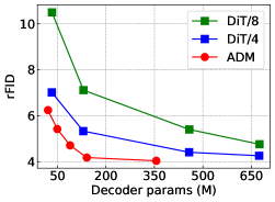
Decoder architecture. We explore two major architectural designs: the UNet-based architecture from ADM (Dhariwal & Nichol, 2021) and the Transformer-based DiT (Peebles & Xie, 2023). We compare various model sizes–ADM:{B, M, L, XL, H} and DiT:{S, B, L, XL} with patch sizes of {4, 8}. The results are summarized in Figure 2 (left). ADM consistently outperforms DiT across the board. While we observe rFID improvements in DiT when increasing the number of tokens by reducing patch size, this comes with significant computational overhead. The overall result aligns with the original design intentions: ADM for pixel-level generation and DiT for latent-level generation. For the following experiments, we use the ADM architecture for our diffusion decoder.
Compression rate. Compression can be achieved by adjusting either the channel dimensions of the latents or the downsampling factor of the encoder. In Figure 2 (middle and right), we compare VAE and -VAE across these two aspects. The results show that -VAE consistently outperforms VAE in terms of rFID, particularly as the compression ratio increases. Specifically, as shown on the middle graph, -VAE achieves lower rFIDs than VAE across all channel dimensions, with a notable gap at lower dimensions (4 and 8). On the right graph, -VAE maintains lower rFIDs than VAE even as the downsampling factor increases, with the gap widening significantly at larger factors (16 and 32). Furthermore, -VAE delivers comparable or superior rFIDs even when the compression ratio is doubled, demonstrating its robustness and effectiveness in high-compression scenarios.
Model scaling. We investigate the impact of model scaling by comparing VAE and -VAE across five model variants, all trained and evaluated at a resolution of , as summarized in Table 1. The results demonstrate that -VAE consistently achieves significantly better rFID scores than VAE, with an average relative improvement of over 40, and even the smallest -VAE model outperforms VAE at largest scale. While the U-Net-based decoder of -VAE has about twice as many parameters as standard decoder of VAE, grouping models by similar sizes, highlighted in blue, red, and green, shows that performance gains are not simply due to increased model parameters.
Resolution generalization. A notable feature of conventional autocencoders is their capacity to generalize and reconstruct images at higher resolutions during inference (Rombach et al., 2022). To assess this, we conduct inference on images with resolutions of and , using -VAE and VAE models trained at . As shown in Table 1, -VAE effectively generalizes to higher resolutions, consistently preserving its performance advantage over VAE.
Runtime efficiency. We examine the inference throughput of the model on a single Tesla V100 GPU. VAE (M) achieves 114.13 images/sec throughput, while the throughput of -VAE (B) is 20.68 images/sec when the sampling step is three and increased to 62.94 images/sec if we sample by one step. -VAE requires more compute costs than VAE due to its U-Net design. We discuss potential directions to improve our runtime efficiency in Sec. 5.
| Models | params (M) | ImageNet | ImageNet † | ImageNet † | |||
|---|---|---|---|---|---|---|---|
| rFID | rFID | rFID | |||||
| VAE (B) | 10.14 | 11.15 | - | 5.74 | - | 3.69 | - |
| VAE (M) | 22.79 | 9.26 | - | 4.63 | - | 2.69 | - |
| VAE (L) | 40.48 | 8.49 | - | 4.78 | - | 2.78 | - |
| VAE (XL) | 65.27 | 7.58 | - | 4.42 | - | 2.41 | - |
| VAE (H) | 161.81 | 7.12 | - | 4.29 | - | 2.37 | - |
| -VAE (B) | 20.63 | 6.24 | 4.91 (44.0) | 3.90 | 1.84 (32.0) | 2.06 | 1.63 (44.2) |
| -VAE (M) | 49.33 | 5.42 | 3.84 (41.5) | 2.79 | 1.84 (39.7) | 2.02 | 0.67 (24.9) |
| -VAE (L) | 88.98 | 4.71 | 3.78 (44.5) | 2.60 | 2.03 (43.8) | 1.92 | 0.86 (30.9) |
| -VAE (XL) | 140.63 | 4.18 | 3.40 (44.9) | 2.38 | 2.04 (46.2) | 1.82 | 0.59 (24.5) |
| -VAE (H) | 355.62 | 4.04 | 3.08 (43.3) | 2.31 | 1.98 (46.2) | 1.78 | 0.59 (24.9) |


| Models | ImageNet | ImageNet | ||||||||
|---|---|---|---|---|---|---|---|---|---|---|
| rFID | FID | IS | Prec. | Rec. | rFID | FID | IS | Prec. | Rec. | |
| VAE (B) | 11.15 | 36.8 | 17.9 | 0.48 | 0.53 | 5.74 | 46.6 | 23.4 | 0.45 | 0.56 |
| VAE (M) | 9.26 | 34.6 | 18.2 | 0.49 | 0.55 | 4.63 | 44.7 | 23.8 | 0.47 | 0.58 |
| VAE (L) | 8.49 | 33.9 | 18.4 | 0.50 | 0.56 | 4.78 | 44.3 | 24.7 | 0.47 | 0.59 |
| VAE (XL) | 7.58 | 31.7 | 19.3 | 0.51 | 0.57 | 4.42 | 43.1 | 24.9 | 0.47 | 0.59 |
| VAE (H) | 7.12 | 30.9 | 19.8 | 0.52 | 0.57 | 4.29 | 41.6 | 25.9 | 0.48 | 0.59 |
| -VAE (B) | 6.24 | 29.5 | 20.7 | 0.53 | 0.59 | 3.90 | 39.5 | 25.2 | 0.46 | 0.61 |
| -VAE (M) | 5.42 | 27.6 | 21.2 | 0.55 | 0.59 | 2.79 | 35.4 | 26.2 | 0.51 | 0.62 |
| -VAE (L) | 4.71 | 27.3 | 22.1 | 0.55 | 0.59 | 2.60 | 34.8 | 26.5 | 0.51 | 0.63 |
| -VAE (XL) | 4.18 | 25.3 | 22.7 | 0.55 | 0.59 | 2.38 | 34.0 | 27.4 | 0.53 | 0.63 |
| -VAE (H) | 4.04 | 24.9 | 23.0 | 0.56 | 0.60 | 2.31 | 33.2 | 27.5 | 0.54 | 0.64 |
4.2 Generation quality
Given the trained VAE and -VAE models, we now evaluate their autoencoding performance. In practice, we first generate latents using the trained autoencoders, then train a new latent generative model based on these representations. The compact, learnable latent space produced by the encoder enhances the learning efficiency of latent generative model, while effective decoding of the sampled latents ensures high-quality outputs. Thus, both the encoding and decoding capabilities of autoencoder contribute to the overall generative performance. For this evaluation, we perform standard unconditional image generation tasks using the DiT-XL/2 model as our latent generative model (Peebles & Xie, 2023). Further details on the training setup are provided in Section B.3.
Table 2 presents the image generation results of VAE and -VAE at resolutions of and . The results show that -VAE consistently outperforms VAE across all model scales. Notably, -VAE (B) surpasses VAE (H), consistent with our earlier findings in Sec. 4.1. These results confirm that the performance gains from the reconstruction task successfully transfer to the generation task, further validating the effectiveness of -VAE.
It is important to note that the primary focus of this experiment is not to achieve state-of-the-art generation results, but to provide a fair comparison of -VAE’s autoencoding capabilities under a controlled experimental setup. We demonstrate that our approach consistently outperforms the leading autoencoding method (Esser et al., 2021) across varying model scales and input resolutions.
4.3 Ablation studies
We conduct a component-wise analysis to validate our key design choices. We evaluate the reconstruction quality (rFID) and sampling efficiency (NFE). The results are summarized in Table 3.
Baseline. Our evaluation begins with a baseline model: an autoencoder with a diffusion decoder, trained solely using the score matching objective. This baseline follows the vanilla diffusion setup from Ho et al. (2020), including their UNet architecture, parameterization, and training configurations, while extending to a conditional form as described in Eq. 8. Building on this baseline, we progressively introduce updates and evaluate the impact of our proposed method.
Impact of proposals. In (1), transitioning from standard diffusion to rectified flow (Liu et al., 2023) straightens the optimization path, resulting in significant gains in rFID scores and NFE. In (2), adopting a logit-normal time step distribution optimizes rectified flow training (Esser et al., 2024), further improving both rFID scores and NFE. In (3), updates to the UNet architecture (Nichol & Dhariwal, 2021) contribute to enhanced rFID scores. In (4), LPIPS loss is applied to match reconstructions with real images . In (5), adversarial trajectory matching loss aligns with , the target transition in rectified flow. Both objectives improve model understanding of the underlying optimization trajectory, significantly enhancing rFID scores and NFE.
Up to this point, with the full implementation of Eq. 1, we can compare our proposal with the VAE (B) model, which achieves an rFID score of 11.15. Our model, with a score of 8.24, already surpasses this baseline. We further improve performance by optimizing noise and time scheduling within our framework, as described next.
In (6), scaling reduces the signal-to-noise ratio (Chen, 2023), presenting challenges for more effective learning during training. Figure 3 (middle) demonstrates that a scaling factor of 0.6 produces the best results. Finally, in (7), reversed logarithmic time step spacing during inference allows for denser evaluations in noisier regions. Figure 3 (right) demonstrates that this method provides more stable sampling in the lower NFE regime compared to the original uniform spacing.
| Ablation | NFE | rFID |
|---|---|---|
| Baseline: DDPM-based diffusion decoder | 1,000 | 28.22 |
| † (1) Diffusion Rectified flow parameterization | 100 | 24.11 |
| § (2) Uniform Logit-normal time step sampling during training | 50 | 23.44 |
| ⋆ (3) DDPM UNet ADM UNet | 50 | 22.04 |
| † (4) Perceptual matching on and | 10 | 11.76 |
| † (5) Adversarial denoising trajectory matching on and | 5 | 8.24 |
| § (6) Scale by | 5 | 7.08 |
| § (7) Uniform Reversed logarithm time spacing during inference | 3 | 6.24 |


5 Discussion
Distribution-aware compression. Traditional image compression methods optimize the rate-distortion trade-off (Shannon et al., 1959), prioritizing compactness over input fidelity. Building on this, we also aim to capture the broader input distribution during compression, generating compact representations suitable for latent generative models. This approach introduces an additional dimension to the trade-off, perception or distribution fidelity (Blau & Michaeli, 2018), which aligns more closely with the rate-distortion-perception framework (Blau & Michaeli, 2019).
Iterative and stochastic decoding. A key question within the rate-distortion-perception trade-off is whether the iterative, stochastic nature of diffusion decoding offers advantages over traditional single-step, deterministic methods (Kingma, 2013). The strengths of diffusion (Ho et al., 2020) lie in its iterative process, which progressively refines the latent space for more accurate reconstructions, while stochasticity allows for capturing complex variations within the distribution. Although iterative methods may appear less efficient, our formulation is optimized to achieve optimal results in just three steps and also supports single-step decoding, ensuring decoding efficiency remains practical (see Figure 3 (left)). While stochasticity might suggest the risk of “hallucination” in reconstructions, the outputs remain faithful to the underlying distribution by design, producing perceptually plausible results. This advantage is particularly evident under extreme compression scenarios (see Figure 4), with the degree of stochasticity adapting based on compression levels (see Figure 5).
Scalability. As discussed in Section 4.1, our diffusion-based decoding method maintains the resolution generalizability typically found in standard autoencoders. This feature is highly practical: the autoencoder is trained on lower-resolution images, while the subsequent latent generative model is trained on latents derived from higher-resolution inputs. However, we acknowledge that memory overhead and throughput become concerns with our UNet-based diffusion decoder, especially for high-resolution inputs. This challenge becomes more pronounced as models, datasets, or resolutions scale up. A promising future direction is patch-based diffusion (Ding et al., 2024; Wang et al., 2024b), which partitions the input into smaller, independently processed patches. This approach has the potential to reduce memory usage and enable faster parallel decoding.


6 Conclusion
We present -VAE, an effective visual tokenization framework that introduces a diffusion decoder into standard autoencoders, turning single-step decoding into a multi-step probabilistic process. By exploring key design choices in modeling, objectives, and diffusion training, we demonstrate significant performance improvements. Our approach outperforms traditional visual autoencoders in both reconstruction and generation quality, particularly in high-compression scenarios. We hope our concept of iterative generation during decoding inspires further advancements in visual autoencoding.
Acknowledgments
We would like to thank Xingyi Zhou, Weijun Wang, and Caroline Pantofaru for reviewing the paper and providing feedback. We thank Rui Qian, Xuan Yang, and Mingda Zhang for helpful discussion. We also thank the Google Kauldron team for technical assistance.
References
- Achiam et al. (2023) Josh Achiam, Steven Adler, Sandhini Agarwal, Lama Ahmad, Ilge Akkaya, Florencia Leoni Aleman, Diogo Almeida, Janko Altenschmidt, Sam Altman, Shyamal Anadkat, et al. GPT-4 technical report. arXiv preprint arXiv:2303.08774, 2023.
- Albergo & Vanden-Eijnden (2023) Michael S Albergo and Eric Vanden-Eijnden. Building normalizing flows with stochastic interpolants. In ICLR, 2023.
- Anil et al. (2023) Rohan Anil, Sebastian Borgeaud, Yonghui Wu, Jean-Baptiste Alayrac, Jiahui Yu, Radu Soricut, Johan Schalkwyk, Andrew M Dai, Anja Hauth, et al. Gemini: a family of highly capable multimodal models. arXiv preprint arXiv:2312.11805, 2023.
- Arjovsky et al. (2017) Martin Arjovsky, Soumith Chintala, and Léon Bottou. Wasserstein generative adversarial networks. In ICML, pp. 214–223, 2017.
- Atchison & Shen (1980) Jhon Atchison and Sheng M Shen. Logistic-normal distributions: Some properties and uses. Biometrika, 67(2):261–272, 1980.
- Baldridge et al. (2024) Jason Baldridge, Jakob Bauer, Mukul Bhutani, Nicole Brichtova, Andrew Bunner, Kelvin Chan, Yichang Chen, Sander Dieleman, Yuqing Du, Zach Eaton-Rosen, et al. Imagen 3. arXiv preprint arXiv:2408.07009, 2024.
- Birodkar et al. (2024) Vighnesh Birodkar, Gabriel Barcik, James Lyon, Sergey Ioffe, David Minnen, and Joshua V Dillon. Sample what you cant compress. arXiv preprint arXiv:2409.02529, 2024.
- Blau & Michaeli (2018) Yochai Blau and Tomer Michaeli. The perception-distortion tradeoff. In CVPR, pp. 6228–6237, 2018.
- Blau & Michaeli (2019) Yochai Blau and Tomer Michaeli. Rethinking lossy compression: The rate-distortion-perception tradeoff. In ICML, pp. 675–685, 2019.
- Bradbury et al. (2018) James Bradbury, Roy Frostig, Peter Hawkins, Matthew James Johnson, Chris Leary, Dougal Maclaurin, George Necula, Adam Paszke, Jake VanderPlas, Skye Wanderman-Milne, and Qiao Zhang. JAX: composable transformations of Python+NumPy programs, 2018. URL http://github.com/jax-ml/jax.
- Brock et al. (2019) Andrew Brock, Jeff Donahue, and Karen Simonyan. Large scale GAN training for high fidelity natural image synthesis. In ICLR, 2019.
- Brooks et al. (2024) Tim Brooks, Bill Peebles, Connor Holmes, Will DePue, Yufei Guo, Li Jing, David Schnurr, Joe Taylor, Troy Luhman, Eric Luhman, Clarence Ng, Ricky Wang, and Aditya Ramesh. Video generation models as world simulators. OpenAI Blog, 2024. URL https://openai.com/research/video-generation-models-as-world-simulators.
- Chang et al. (2022) Huiwen Chang, Han Zhang, Lu Jiang, Ce Liu, and William T Freeman. MaskGIT: Masked generative image transformer. In CVPR, pp. 11315–11325, 2022.
- Chen et al. (2020) Mark Chen, Alec Radford, Rewon Child, Jeffrey Wu, Heewoo Jun, David Luan, and Ilya Sutskever. Generative pretraining from pixels. In ICML, pp. 1691–1703, 2020.
- Chen (2023) Ting Chen. On the importance of noise scheduling for diffusion models. arXiv preprint arXiv:2301.10972, 2023.
- Chen et al. (2023) Ting Chen, Lala Li, Saurabh Saxena, Geoffrey Hinton, and David J Fleet. A generalist framework for panoptic segmentation of images and videos. In ICCV, pp. 909–919, 2023.
- Deng et al. (2009) Jia Deng, Wei Dong, Richard Socher, Li-Jia Li, Kai Li, and Li Fei-Fei. ImageNet: A large-scale hierarchical image database. In CVPR, pp. 248–255, 2009.
- Dhariwal & Nichol (2021) Prafulla Dhariwal and Alexander Nichol. Diffusion models beat GANs on image synthesis. In NeurIPS, 2021.
- Ding et al. (2024) Zheng Ding, Mengqi Zhang, Jiajun Wu, and Zhuowen Tu. Patched denoising diffusion models for high-resolution image synthesis. In ICLR, 2024.
- Dubey et al. (2024) Abhimanyu Dubey, Abhinav Jauhri, Abhinav Pandey, Abhishek Kadian, Ahmad Al-Dahle, Aiesha Letman, Akhil Mathur, Alan Schelten, Amy Yang, Angela Fan, et al. The Llama 3 Herd of Models. arXiv preprint arXiv:2407.21783, 2024.
- Esser et al. (2021) Patrick Esser, Robin Rombach, and Bjorn Ommer. Taming transformers for high-resolution image synthesis. In CVPR, pp. 12873–12883, 2021.
- Esser et al. (2024) Patrick Esser, Sumith Kulal, Andreas Blattmann, Rahim Entezari, Jonas Müller, Harry Saini, Yam Levi, Dominik Lorenz, Axel Sauer, Frederic Boesel, Dustin Podell, Tim Dockhorn, Zion English, Kyle Lacey, Alex Goodwin, Yannik Marek, and Robin Rombach. Scaling rectified flow transformers for high-resolution image synthesis. In ICML, 2024.
- Euler (1845) Leonhard Euler. Institutionum calculi integralis, volume 4. impensis Academiae imperialis scientiarum, 1845.
- Goodfellow et al. (2014) Ian Goodfellow, Jean Pouget-Abadie, Mehdi Mirza, Bing Xu, David Warde-Farley, Sherjil Ozair, Aaron Courville, and Yoshua Bengio. Generative adversarial nets. In NeurIPS, 2014.
- Gupta et al. (2023) Agrim Gupta, Lijun Yu, Kihyuk Sohn, Xiuye Gu, Meera Hahn, Li Fei-Fei, Irfan Essa, Lu Jiang, and José Lezama. Photorealistic video generation with diffusion models. arXiv preprint arXiv:2312.06662, 2023.
- Heek et al. (2024) Jonathan Heek, Anselm Levskaya, Avital Oliver, Marvin Ritter, Bertrand Rondepierre, Andreas Steiner, and Marc van Zee. Flax: A neural network library and ecosystem for JAX, 2024. URL http://github.com/google/flax.
- Heusel et al. (2017) Martin Heusel, Hubert Ramsauer, Thomas Unterthiner, Bernhard Nessler, and Sepp Hochreiter. GANs Trained by a Two Time-Scale Update Rule Converge to a Local Nash Equilibrium. In NeurIPS, 2017.
- Hinton & Salakhutdinov (2006) Geoffrey E Hinton and Ruslan R Salakhutdinov. Reducing the dimensionality of data with neural networks. Science, 313(5786):504–507, 2006.
- Ho & Salimans (2022) Jonathan Ho and Tim Salimans. Classifier-free diffusion guidance. arXiv preprint arXiv:2207.12598, 2022.
- Ho et al. (2020) Jonathan Ho, Ajay Jain, and Pieter Abbeel. Denoising diffusion probabilistic models. In NeurIPS, 2020.
- Ho et al. (2022) Jonathan Ho, Chitwan Saharia, William Chan, David J Fleet, Mohammad Norouzi, and Tim Salimans. Cascaded diffusion models for high fidelity image generation. Journal of Machine Learning Research, 23(47):1–33, 2022.
- Hoogeboom et al. (2023a) Emiel Hoogeboom, Eirikur Agustsson, Fabian Mentzer, Luca Versari, George Toderici, and Lucas Theis. High-fidelity image compression with score-based generative models. arXiv preprint arXiv:2305.18231, 2023a.
- Hoogeboom et al. (2023b) Emiel Hoogeboom, Jonathan Heek, and Tim Salimans. simple diffusion: End-to-end diffusion for high resolution images. In ICML, pp. 13213–13232, 2023b.
- Karras et al. (2019) Tero Karras, Samuli Laine, and Timo Aila. A style-based generator architecture for generative adversarial networks. In CVPR, pp. 4401–4410, 2019.
- Karras et al. (2022) Tero Karras, Miika Aittala, Timo Aila, and Samuli Laine. Elucidating the design space of diffusion-based generative models. In NeurIPS, 2022.
- Kingma & Gao (2024) Diederik Kingma and Ruiqi Gao. Understanding diffusion objectives as the elbo with simple data augmentation. In NeurIPS, 2024.
- Kingma (2013) Diederik P Kingma. Auto-encoding variational bayes. arXiv preprint arXiv:1312.6114, 2013.
- Kingma & Ba (2015) Diederik P. Kingma and Jimmy Ba. Adam: A method for stochastic optimization. In ICLR, 2015.
- Kondratyuk et al. (2024) Dan Kondratyuk, Lijun Yu, Xiuye Gu, José Lezama, Jonathan Huang, Rachel Hornung, Hartwig Adam, Hassan Akbari, Yair Alon, Vighnesh Birodkar, et al. VideoPoet: A large language model for zero-shot video generation. In ICML, 2024.
- Kudo (2018) Taku Kudo. Subword regularization: Improving neural network translation models with multiple subword candidates. arXiv preprint arXiv:1804.10959, 2018.
- Kudo & Richardson (2018) Taku Kudo and John Richardson. Sentencepiece: A simple and language independent subword tokenizer and detokenizer for neural text processing. arXiv preprint arXiv:1808.06226, 2018.
- Kynkäänniemi et al. (2019) Tuomas Kynkäänniemi, Tero Karras, Samuli Laine, Jaakko Lehtinen, and Timo Aila. Improved precision and recall metric for assessing generative models. In NeurIPS, 2019.
- Lee et al. (2024) Sangyun Lee, Zinan Lin, and Giulia Fanti. Improving the training of rectified flows. arXiv preprint arXiv:2405.20320, 2024.
- Li et al. (2024) Tianhong Li, Yonglong Tian, He Li, Mingyang Deng, and Kaiming He. Autoregressive image generation without vector quantization. arXiv preprint arXiv:2406.11838, 2024.
- Lipman et al. (2022) Yaron Lipman, Ricky TQ Chen, Heli Ben-Hamu, Maximilian Nickel, and Matt Le. Flow matching for generative modeling. In ICLR, 2022.
- Liu et al. (2023) Xingchao Liu, Chengyue Gong, and Qiang Liu. Flow straight and fast: Learning to generate and transfer data with rectified flow. In ICLR, 2023.
- Ma et al. (2024) Nanye Ma, Mark Goldstein, Michael S Albergo, Nicholas M Boffi, Eric Vanden-Eijnden, and Saining Xie. Sit: Exploring flow and diffusion-based generative models with scalable interpolant transformers. arXiv preprint arXiv:2401.08740, 2024.
- Mescheder et al. (2018) Lars Mescheder, Andreas Geiger, and Sebastian Nowozin. Which training methods for GANs do actually converge? In ICML, pp. 3481–3490, 2018.
- Nichol & Dhariwal (2021) Alexander Quinn Nichol and Prafulla Dhariwal. Improved denoising diffusion probabilistic models. In ICML, pp. 8162–8171, 2021.
- Peebles & Xie (2023) William Peebles and Saining Xie. Scalable diffusion models with transformers. In ICCV, pp. 4195–4205, 2023.
- Perez et al. (2018) Ethan Perez, Florian Strub, Harm De Vries, Vincent Dumoulin, and Aaron Courville. FiLM: Visual reasoning with a general conditioning layer. In AAAI, 2018.
- Radford et al. (2018) Alec Radford, Karthik Narasimhan, Tim Salimans, and Ilya Sutskever. Improving language understanding by generative pre-training. OpenAI Blog, 2018.
- Razavi et al. (2019) Ali Razavi, Aaron Van den Oord, and Oriol Vinyals. Generating diverse high-fidelity images with VQ-VAE-2. In NeurIPS, 2019.
- Rombach et al. (2022) Robin Rombach, Andreas Blattmann, Dominik Lorenz, Patrick Esser, and Björn Ommer. High-resolution image synthesis with latent diffusion models. In CVPR, pp. 10684–10695, 2022.
- Sadat et al. (2024) Seyedmorteza Sadat, Jakob Buhmann, Derek Bradley, Otmar Hilliges, and Romann M Weber. LiteVAE: Lightweight and efficient variational autoencoders for latent diffusion models. arXiv preprint arXiv:2405.14477, 2024.
- Saharia et al. (2022a) Chitwan Saharia, William Chan, Huiwen Chang, Chris Lee, Jonathan Ho, Tim Salimans, David Fleet, and Mohammad Norouzi. Palette: Image-to-image diffusion models. In ACM SIGGRAPH, pp. 1–10, 2022a.
- Saharia et al. (2022b) Chitwan Saharia, Jonathan Ho, William Chan, Tim Salimans, David J Fleet, and Mohammad Norouzi. Image super-resolution via iterative refinement. IEEE TPAMI, 45(4):4713–4726, 2022b.
- Salimans et al. (2016) Tim Salimans, Ian Goodfellow, Wojciech Zaremba, Vicki Cheung, Alec Radford, and Xi Chen. Improved techniques for training GANs. In NeurIPS, 2016.
- Sennrich et al. (2015) Rico Sennrich, Barry Haddow, and Alexandra Birch. Neural machine translation of rare words with subword units. arXiv preprint arXiv:1508.07909, 2015.
- Shannon et al. (1959) Claude E Shannon et al. Coding theorems for a discrete source with a fidelity criterion. IRE Nat. Conv. Rec, 4(142-163):1, 1959.
- Simonyan & Zisserman (2015) Karen Simonyan and Andrew Zisserman. Very deep convolutional networks for large-scale image recognition. In ICLR, 2015.
- Song & Ermon (2019) Yang Song and Stefano Ermon. Generative modeling by estimating gradients of the data distribution. In NeurIPS, 2019.
- Song et al. (2021) Yang Song, Jascha Sohl-Dickstein, Diederik P Kingma, Abhishek Kumar, Stefano Ermon, and Ben Poole. Score-based generative modeling through stochastic differential equations. In ICLR, 2021.
- Van den Oord et al. (2016) Aaron Van den Oord, Nal Kalchbrenner, Lasse Espeholt, Oriol Vinyals, Alex Graves, et al. Conditional image generation with pixelcnn decoders. In NeurIPS, 2016.
- Van Den Oord et al. (2017) Aaron Van Den Oord, Oriol Vinyals, et al. Neural discrete representation learning. In NeurIPS, 2017.
- Wang et al. (2024a) Fu-Yun Wang, Zhaoyang Huang, Alexander William Bergman, Dazhong Shen, Peng Gao, Michael Lingelbach, Keqiang Sun, Weikang Bian, Guanglu Song, Yu Liu, et al. Phased consistency model. arXiv preprint arXiv:2405.18407, 2024a.
- Wang et al. (2024b) Zhendong Wang, Yifan Jiang, Huangjie Zheng, Peihao Wang, Pengcheng He, Zhangyang ”Atlas” Wang, Weizhu Chen, and Mingyuan Zhou. Patch diffusion: Faster and more data-efficient training of diffusion models. In NeurIPS, 2024b.
- Wu & He (2018) Yuxin Wu and Kaiming He. Group normalization. In ECCV, pp. 3–19, 2018.
- Xiao et al. (2022) Zhisheng Xiao, Karsten Kreis, and Arash Vahdat. Tackling the generative learning trilemma with denoising diffusion GANs. In ICLR, 2022.
- Yang & Mandt (2024) Ruihan Yang and Stephan Mandt. Lossy image compression with conditional diffusion models. In NeurIPS, 2024.
- Yu et al. (2022) Jiahui Yu, Xin Li, Jing Yu Koh, Han Zhang, Ruoming Pang, James Qin, Alexander Ku, Yuanzhong Xu, Jason Baldridge, and Yonghui Wu. Vector-quantized image modeling with improved VQGAN. In ICLR, 2022.
- Yu et al. (2023) Lijun Yu, Yong Cheng, Kihyuk Sohn, José Lezama, Han Zhang, Huiwen Chang, Alexander G Hauptmann, Ming-Hsuan Yang, Yuan Hao, Irfan Essa, et al. MAGVIT: Masked generative video transformer. In CVPR, pp. 10459–10469, 2023.
- Yu et al. (2024a) Lijun Yu, José Lezama, Nitesh B Gundavarapu, Luca Versari, Kihyuk Sohn, David Minnen, Yong Cheng, Agrim Gupta, Xiuye Gu, Alexander G Hauptmann, et al. Language model beats diffusion–tokenizer is key to visual generation. In ICLR, 2024a.
- Yu et al. (2024b) Qihang Yu, Mark Weber, Xueqing Deng, Xiaohui Shen, Daniel Cremers, and Liang-Chieh Chen. An image is worth 32 tokens for reconstruction and generation. arXiv preprint arXiv:2406.07550, 2024b.
- Zhang et al. (2018) Richard Zhang, Phillip Isola, Alexei A Efros, Eli Shechtman, and Oliver Wang. The unreasonable effectiveness of deep features as a perceptual metric. In CVPR, pp. 586–595, 2018.
- Zhao et al. (2024) Yue Zhao, Yuanjun Xiong, and Philipp Krähenbühl. Image and video tokenization with binary spherical quantization. arXiv preprint arXiv:2406.07548, 2024.
Appendix A Related work
Image tokenization. Image tokenization is crucial for effective generative modeling, transforming images into compact, structured representations. A common approach employs an autoencoder framework (Hinton & Salakhutdinov, 2006), where the encoder compresses images into low-dimensional latent representations, and the decoder reconstructs the original input. These latent representations can be either discrete commonly used in autoregressive models (Van den Oord et al., 2016; Van Den Oord et al., 2017; Chen et al., 2020; Chang et al., 2022; Yu et al., 2023; Kondratyuk et al., 2024), or continuous, as found in diffusion models (Ho et al., 2020; Dhariwal & Nichol, 2021; Rombach et al., 2022; Peebles & Xie, 2023; Gupta et al., 2023; Brooks et al., 2024). The foundational form of visual autoencoding today originates from Van Den Oord et al. (2017). While advancements have been made in modeling (Yu et al., 2022; 2024b), objectives (Zhang et al., 2018; Karras et al., 2019; Esser et al., 2021), and quantization methods (Yu et al., 2024a; Zhao et al., 2024), the core encoding-and-decoding scheme remains largely the same.
In this work, we propose a new perspective by replacing the traditional decoder with a diffusion process. Specifically, our new formulation retains the encoder but introduces a conditional diffusion decoder. Within this framework, we systematically study various design choices, resulting in a significantly enhanced autoencoding setup.
Additionally, we refer to the recent work MAR (Li et al., 2024), which leverages diffusion to model per-token distribution in autoregressive frameworks. In contrast, our approach models the overall input distribution in autoencoders using diffusion. This difference leads to distinct applications of diffusion during generation. For instance, MAR generates samples autoregressively, decoding each token iteratively using diffusion, token by token. In our method, we first sample all tokens from the downstream generative model and then decode them iteratively using diffusion as a whole.
Image compression. Our work shares similarities with recent image compression approaches that leverage diffusion models. For example, Hoogeboom et al. (2023a); Birodkar et al. (2024) use diffusion to refine autoencoder residuals, enhancing high-frequency details. Yang & Mandt (2024) employs a diffusion decoder conditioned on quantized discrete codes and omits the GAN loss. However, these methods primarily focus on the traditional rate-distortion tradeoff, balancing rate (compactness) and distortion (input fidelity) (Shannon et al., 1959), with the goal of storing and transmitting data efficiently without significant loss of information.
In this work, we emphasize perception (distribution fidelity) alongside the rate-distortion tradeoff, ensuring that reconstructions more closely align with the overall data distribution (Heusel et al., 2017; Zhang et al., 2018; Blau & Michaeli, 2019), thereby enhancing the decoded results from the sampled latents of downstream generative models. We achieve this by directly integrating the diffusion process into the decoder, unlike Hoogeboom et al. (2023a); Birodkar et al. (2024). Moreover, unlike Yang & Mandt (2024), we do not impose strict rate-distortion regularization in the latent space and allow the GAN loss to synergize with our approach.
Image generation. Recent advances in image generation span a wide range of approaches, including VAEs (Kingma, 2013), GANs (Goodfellow et al., 2014), autoregressive models (Chen et al., 2020) and diffusion models (Song et al., 2021; Ho et al., 2020). Among these, diffusion models have emerged as the leading approach for generating high-dimensional data such as images (Saharia et al., 2022a; Baldridge et al., 2024; Esser et al., 2024) and videos (Brooks et al., 2024; Gupta et al., 2023), where the gradual refinement of global structure is crucial. The current focus in diffusion-based generative models lies in advancing architectures (Rombach et al., 2022; Peebles & Xie, 2023; Hoogeboom et al., 2023b), parameterizations (Karras et al., 2022; Kingma & Gao, 2024; Ma et al., 2024; Esser et al., 2024), or better training dynamics (Nichol & Dhariwal, 2021; Chen, 2023; Chen et al., 2023). However, tokenization, an essential component in modern diffusion models, often receives less attention.
In this work, we focus on providing compact continuous latents without applying quantization during autoencoder training (Rombach et al., 2022), as they have been shown to be effective in state-of-the-art latent diffusion models (Rombach et al., 2022; Saharia et al., 2022a; Peebles & Xie, 2023; Esser et al., 2024; Baldridge et al., 2024). We compare our autoencoding performance against the baseline approach (Esser et al., 2021) using the DiT framework (Peebles & Xie, 2023) as the downstream generative model.
Appendix B Experiment setups
In this section, we provide additional details on our experiment configurations for reproducibility.
B.1 Model specifications
Table 4 summarizes the primary architecture details for each decoder variant. The channel dimension is the number of channels of the first U-Net layer, while the depth multipliers are the multipliers for subsequent resolutions. The number of residual blocks denotes the number of residual stacks contained in each resolution.
| Models | Channel dim. | Depth multipliers | # Residual blocks |
|---|---|---|---|
| Base (B) | 64 | {1, 1, 2, 2, 4} | 2 |
| Medium (M) | 96 | {1, 1, 2, 2, 4} | 2 |
| Large (L) | 128 | {1, 1, 2, 2, 4} | 2 |
| Extra-large (XL) | 128 | {1, 1, 2, 2, 4} | 4 |
| Huge (H) | 256 | {1, 1, 2, 2, 4} | 2 |
B.2 Additional implementation details
During the training of discriminators, Esser et al. (2021) introduced an adaptive weighting strategy for . However, we notice that this adaptive weighting does not introduce any benefit which is consistent with the observation made by Sadat et al. (2024). Thus, we set in the experiments for more stable model training across different configurations.
B.3 Latent diffusion model
We follow the setting in Peebles & Xie (2023) to train the latent diffusion models for unconditional image generation on the ImageNet dataset. The DiT-XL/2 architecture is used for all experiments. The diffusion hyperparameters from ADM (Dhariwal & Nichol, 2021) are kept. To be specific, we use a linear variance schedule ranging from 0.0001 to 0.02, and results are generated using 250 DDPM sampling steps. All models are trained with Adam (Kingma & Ba, 2015) with no weight decay. We use a constant learning rate of 0.0001 and a batch size of 256. Horizontal flipping and random cropping are used for data augmentation. We maintain an exponential moving average of DiT weights over training with a decay of 0.9999. We use identical training hyperparameters across all experiments and train models for one million steps in total. No classifier-free guidance (Ho & Salimans, 2022) is employed since we target unconditional generation.
Appendix C Additional experimental results
| Configurations | NFE | rFID |
| Baseline (3) in Table 3: | ||
| Inject conditioning by channel-wise concatenation | 50 | 22.04 |
| Inject conditioning by AdaGN | 50 | 22.01 |
| Baseline (5) in Table 3: | ||
| Matching the distribution of and | - | N/A |
| Matching the trajectory of | 5 | 8.24 |
| Matching the trajectory of | 5 | 10.53 |
Conditioning. In addition to injecting conditioning via channel-wise concatenation, we explore providing conditioning to the diffusion model by adaptive group normalization (AdaGN) (Nichol & Dhariwal, 2021; Dhariwal & Nichol, 2021). To achieve this, we resize the conditioning (i.e., encoded latents) via bilinear sampling to the desired resolution of each stage in the U-Net model, and incorporates it into each residual block after a group normalization operation (Wu & He, 2018). This is similar to adaptive instance norm (Karras et al., 2019) and FiLM (Perez et al., 2018). We report the results in Table 5 (top), where we find that channel-wise concatenation and AdaGN obtain similar reconstruction quality in terms of rFID. Because of the additional computational cost required by AdaGN, we thus apply channel-wise concatenation in our model by default.
Trajectory matching. The proposed denoising trajectory matching objective matches the start-to-end trajectory by default. One alternative choice is to directly matching the distribution of and without coupling on . However, we find this formulation leads to unstable training and could not produce reasonable results. Here, we present the results when matching the trajectory of , which is commonly used in previous work (Xiao et al., 2022; Wang et al., 2024a). Specifically, for each timestep during training, we randomly sample a step from . Then, we construct the real trajectory by computing via Eq. 5 and concatenating it with , while the fake trajectory is obtained in a similar way but using Eq. 10 instead. Table 5 (bottom) shows the comparison. We observe that matching trajectory yields better performance than matching trajectory , confirming the effectiveness of the proposed objective which is designed for the rectified flow formulation.
Qualitative reconstructions. Figure 6 provides qualitative reconstruction results where we vary the decoder scales. We see that increasing the scale of the model yields significant improvements in visual fidelity, and -VAE outperforms VAE at corresponding decoder scales. Figure 7 and Figure 8 show additional qualitative results when we vary the downsampling ratios and random seeds.


