Blowups and Tops of Overlapping Iterated Function Systems
Abstract
We review aspects of an important paper by Robert Strichartz concerning reverse iterated function systems (i.f.s.) and fractal blowups. We compare the invariant sets of reverse i.f.s. with those of more standard i.f.s. and with those of inverse i.f.s. We describe Strichartz’ fractal blowups and explain how they may be used to construct tilings of even in the case where the i.f.s. is overlapping. We introduce and establish the notion of “tops” of blowups. Our motives are not pure: we seek to show that a simple i.f.s. and an idea of Strichartz, can be used to create complicated tilings that may model natural structures.
Dedicated to Robert Strichartz

1 Introduction
In “Fractals in the large” strichartz Robert Strichartz observes that fractal structure is characterized by repetition of detail at all small scales. He asks “Why not large scales as well?” He proposes two ways to study large scaling structures using developments of iterated function systems. Here we review geometrical aspects of his paper and make a contribution in the area of tiling theory.
In his first approach, Strichartz defines a reverse iterated function system (r.i.f.s.) to be a set of expansive maps
acting on a locally compact discrete metric space , where every point of is isolated. Here the large scaling structures are the invariant sets of , sets which obey
Why does does Strichartz restrict his definition to functions acting on discrete metric spaces? (i) He establishes that there are interesting nontrivial examples. (ii) He shows that such objects (act as a kind of skeleton to) play a role in his second kind of large scale fractal structure that he calls a fractal blowup. Probably he had other reasons related to situations where his approach to analysis on fractals could be explored.
In Section 2 we present notation for iterated function systems (i.f.s.) acting on . We are particularly concerned with notation for chains of compositions of functions and properties of addresses of points on fractals. In Section 3 we review Strichartz’ definition and basic theorem concerning invariant sets of reverse iterated function systems, and we compare them to the corresponding situation for contractive i.f.s. We describe some kinds of invariant sets of contractive i.f.s. and consider how they compare to Strichartz’ large scaling structures. It is a notable feature of Strichartz’ definition that he restricts attention to functions acting on compact discrete metric spaces. We mention that, if this restriction is lifted, sometimes very interesting structures, characterized by repetition of structure at large scales, may be obtained. See for example Figure 2.
In Section 4 we define fractal blowups, Strichartz’ second kind of large scale fractal structure, and present his characterization of them, when the open set condition (OSC) is obeyed, as unions of scaled copies of an i.f.s. attractor, with the scaling restricted to a finite range. We outline the proof of his characterization theorem using different notation, anticipating fractal tops. We recall Strichartz’ final theorem on the topic, where he restricts attention to blowups of an i.f.s. all of the same scaling factor. Here he combines his two ideas: he reveals that the fractal blowup is in fact a copy of the original fractal translated by all the points on an invariant set of a r.i.f.s.
In Section 5 we discuss how tilings of blowups can be extended to overlapping i.f.s. In tilings it was shown how, in the overlapping (OSC not obeyed) case, tilings of blowups can be defined using an artificial recursive system of “masks”. Here the approach is more natural, but we pay a price–sequences of tilings are not necessarily nested. Here tilings are defined by using “fractal tops”, namely attractors with their points labelled by lexicographically highest addresses. The needed theory of fractal tops is developed in Subsection 5.1. Then in Subsection 5.2 we use these top addresses to define and establish the existence of tilings of some blowups for overlapping i.f.s. The main theorem concerns the relationship between the successive tilings that may be used to define a tiling of a blowup. In Subsection 5.3 we present an example involving a tile that resembles a leaf.
Strichartz’ paper has overlap with bandt2 , published about the same time by Christoph Bandt. Both papers consider the relationship between i.f.s. theory and self-similar tiling theory. Current work in tiling theory does not typically use the mapping point of view, but both Bandt and Stricharz do. Bandt is particularly focused on the open set condition and the algebraic structure of tilings, but also has a clear understanding of tilings of blowups when the OSC is obeyed.
Strichartz’ paper also contains measure theory aspects that we do not discuss. But from the little we have focused on here, much has been learned concerning the subtlety, the depth, and the elegant simplicity of the mathematical thinking of Robert Strichartz.
2 Preliminaries
Let An iterated function system (i.f.s.) is a set of functions
mapping a space into itself, with . An invariant set of is such that
We use the same symbol for the i.f.s. and for its action on , as defined here.
The i.f.s. is said to be contractive when is equipped with a metric such that for some and all . If we take to be the Euclidean metric. A contractive i.f.s. on is associated with its attractor , the unique non-empty closed and bounded invariant set of hutchinson . But Strichartz is also interested in the case where the underlying space is discrete and the maps are expansive.
We use addresses to describe compositions of maps. Addresses are defined in terms of the indices of the maps of . Let , the set of strings of the form where each belongs to . We write and let The address truncated to length is denoted by and we define
Define a metric on by for , so that is a compact metric space.
The forward orbit of a point under (the semigroup generated by) is
Here we do not allow to be the empty set, so is not necessarily an element of its forward orbit under the i.f.s. Indeed, is a member of its forward orbit if and only if is a fixed point of one of the composite maps .
Now let be a contractive IFS of invertible maps on . Then a continuous surjection is defined by
The limit is independent of . The convergence is uniform in over and uniform in over any compact subset of . We say is an address of the point .
We define by But we may also write to mean the address Let be the shift operator defined by . It is well-known that
for all .
A notable shift invariant subset of is the set of disjunctive addresses . An address is disjunctive when, for each finite address , there is so that . The set of disjunctive addresses is totally invariant under the shift, according to A point is disjunctive if there is a disjunctive address such that . Disjunctive points play a role in the structure of attractors. For example, if the i.f.s. obeys the open set condition (OSC) and its attractor has non-empty interior, then all the disjunctive points belong to the interior of the attractor bandt . Recall that obeys the OSC when there exists a nonempty open set such that and whenever
3 Reverse iterated function systems
In his first approach to large scaling structures, Strichartz defines a reverse iterated function system (r.i.f.s.) to be a set of expansive maps
acting on a locally compact discrete (i.e. every point is isolated) metric space . We write and in place of and to distinguish this special kind of i.f.s. A mapping is said to be expansive if there is a constant such that for all in An expansive mapping is necessarily one-to-one and has at most one fixed point.
In this case Strichartz’s large scaling structures are the invariant sets of r.i.f.s.; that is, sets which obey
By requiring that is discrete, Strichartz restricts the possible invariant sets to be discrete.
Theorem 3.1 (Strichartz)
A set is invariant for a r.i.f.s. if and only if it is a finite union of forward orbits of points in . In particular, invariant sets exist if and only if is nonempty, and there are at most a finite number of invariant sets.
EXAMPLE 1 Let , It is readily verified that is invariant for this r.i.f.s, It consists of the forward orbits of the fixed points of and
EXAMPLE 2 Strichartz presents the following example of a r.i.f.s. Let be the set of integer lattice points in the plane, lying between or on the lines and where The r.i.f.s. comprises the two maps
These maps are expansive on , even though when viewed as transformations acting on they contract pairs of points that lie on any straight line with slope . The fixed point of is and of is both of which lie in The union of the forward orbits of these two points is . So this unlikely looking set of discrete points is invariant under the r.i.f.s.
This example yields, by projection onto the line an example of a quasi-periodic linear tiling using tiles of lengths and Strichartz also points out that by projection onto the perpendicular line of a natural measure on one obtains, after renormalizing, the unique self-similar measure on associated with the overlapping i.f.s. , with equal probabilities.
Theorem 3.1 leads one to wonder: What are the invariant sets of an i.f.s.? Usually the focus is on compact invariant sets, namely attractors. The following Theorem is simply a list of some of the invariant sets of a contractive i.f.s. The wealth of such invariants here stands in sharp contrast to Theorem 3.1.
Theorem 3.2 (Some Invariant Sets of an i.f.s.)
Let be a contractive i.f.s. of invertible maps on If is invariant and bounded, then either or The followings sets are invariant.
-
1.
The attractor and the whole space
-
2.
The forward orbit under of any periodic point
-
3.
The set of disjunctive points of .
-
4.
The orbit of any under the free group generated by the maps of and their inverses.
-
5.
The union of any collection of invariant sets.
There are other invariant sets. For example, let be a Sierpinski triangle, the attractor of an i.f.s. in the usual way. Let be the union of the sides of all triangles in Then is an invariant set for . It is not covered by Theorem 3.2.
We note that the invariant set in (4) is also invariant under the inverse i.f.s.
The orbit under of the attractor is invariant under This set may be referred to as the fast basin of with respect to , see fastbasin . It is an example of a set which is “invariant in the large”, admitted when Strichartz’ constraint, that the underlying space is discrete and locally compact, is lifted.
Figure 2 illustrates the fast basin associated with (left) a Sierpinski triangle i.f.s. and (right) a different i.f.s. of three similitudes of scaling factor Fast basins are interesting from a computational point of view, because they comprise the points in for which there is an address such that .

4 Strichartz’ fractal blowups
Strichartz uses r.i.f.s. to analyze the structure of what he christened “fractal blowups”. These structures have been used to develop differential operators on unbounded fractals, see for example strichartz2 ; teplyaev .
Let be an i.f.s. of similitudes. The maps take the form
where and is an orthogonal transformation. It is convenient to write where , so that . A blowup of is the union of an increasing sequence of sets
| (1) |
where for some fixed and all . We have
| (2) |
Strichartz starts with a more general definition of a blowup, but restricts consideration to the one given here.
Theorem 4.1 (Strichartz)
Let be a blowup of of the form in Equation (2) and assume satisfies the OSC. Then is the union of sets which are similar to with the contraction ratios bounded from above and below, and the number of sets that intersect any ball of radius is at most a multiple of In particular the union is locally finite, and the intersection of with any compact set is equal to the intersection of with that compact set for large .
Proof
We outline a proof for the case of a single scaling factor with . At heart, our proof is the same as Strichartz, but we introduce notation that helps with our generalization to overlapping i.f.s. in Section 5.
Since satisfies the OSC, there is a bounded open set such that for all for all Note that the latter condition implies that the sets in are disjoint.
Define a collection of sets
where may be , or Observe that
and
Also
consists of disjoint open sets. It follows that is a nested increasing sequence of disjoint open sets, whose closed union contains . The closure of each open set contains a copy of Since each open set has volume bounded below by a positive constant, local finiteness is assured.
A general case of a Strichartz style blowup is captured by defining
where
These formulas provide a specific form to Strichartz’ stopping time argument. Using these more general expressions one obtains, for fixed , an increasing union of copies of scaled by factors that lie between and See for example tilings ; polygon . The argument concerning local finiteness is essentially the same as above.
Strichartz unites his two ideas, reverse i.f.s. and blowups, by considering the case where for all and studying the blowup where that is
Theorem 4.2 (Strichartz combines r.i.f.s. and blowups)
Let Then where is an invariant set for the r.i.f.s.
Specifically, is the forward orbit of , the fixed point of
That is, is the Minkowski sum of the attractor of the i.f.s. and an invariant set of a r.i.f.s.
5 Tops tilings
In this Section we study tilings of fractal blowups in the case of overlapping i.f.s. attractors. First, in Subsection 5.1 we give relevant theory of fractal tops. In Subsection 5.2 we show how fractal tops may be used to generate tilings of fractal blowups for overlapping i.f.s. The approach here is distinct from the one in tilings . In Subsection 5.3 we illustrate fractal tops for an i.f.s. of two maps, with overlapping attractor that looks like a leaf, suggesting applications to modelling of complicated real-world images.
5.1 Fractal tops
Let be a strictly contractive i.f.s. acting on a complete metric space , with maps and attractor We assume that there are two or more maps, at least two of which have different fixed points. Also all of the maps are invertible.
Lemma 1
Let be a closed subset of Let Then
Proof
is the union of the three closed sets , and The maximum over is the maximum of the maxima over these three sets. But the set is empty, because if not then which is a contradiction. If then , again a contradiction.
Since is continuous and onto, it follows that is closed for all Lemma 1 tells us that a map and subset are well-defined by
Conventionally the maximum here is with respect to lexicographical ordering. We refer loosely to these objects and the ideas around them as relating to the top of Formally, the top of is the graph of namely .
Top addresses of points in namely points in can be calculated by following the orbits of the shift map Simply partition into . Define the orbit of under the tops dynamical system, by where is the unique index such that .
Theorem 5.1
The set of top addresses is shift invariant, according to where is the left shift.
Proof
First we show that If then
Hence Hence which implies
We also have so But by a similar argument to the proof of Lemma 1, so Applying to both sides, we obtain
It appears that the shift space is not of finite type in general, and graph directed constructions cannot be used in general. This is a topic of ongoing research.
Define to be the elements of truncated to the first elements. That is,
Define to be the restriction of to Extend the definition of so that it acts on truncated top addresses according to:
for all and all . We will make use of the following observation.
Lemma 2
If then for all .
Proof
We need to compare the sets
and
The condition in the latter expression is less restrictive.
The sets of truncated top addresses have an interesting structure. Any addresses in can be truncated on the left or on the right to obtain an address in The following Lemma is readily verified.
Lemma 3
Let If , then both and belong to
5.2 Top blowups and tilings
Here we are particularly interested in the overlapping case, where the OSC does not hold. We show that natural partitions of fractal blowups, that we call tilings, may still be obtained.
Throughout this subsection, is an i.f.s. with
| (3) |
where and is an orthogonal transformation. We assume that there are two or more maps, at least two of which have distinct fixed points. We have in mind the situation where is homeomorphic to a ball, although this is not required by Theorems 5.2 and 5.3.
As in Section 4, but restricted to fractal blowups are well defined by
The unions are of increasing nested sequences of sets so and Note that is related to by the isometry . But possible relationships between and are quite subtle because inverse limits are involved.
Under conditions on and , stated in Theorems 5.2 and 5.3, we can define a generalized tilings of with the aid of the following two definitions:
For example, the limit is well defined when for all as occurs when the OSC holds. As we will show, it is also well defined in some more complicated situations.
We call each set a tile, and we call the collection of disjoint sets a partial tiling. The partial tilings are well defined. However, may not be well defined, because there may not be any simple relationship between successive partial tilings. But when it is well defined, we call it a tiling.
The tiles in the partial tiling may be referred to by their addresses. It is convenient to define
for all and all We also define corresponding to
Lemma 4
This concerns the sequence of tilings If then implies .
Proof
Suppose Then applying to both sides we obtain which is equivalent to
But by Lemma 2, so
This implies because otherwise and are disjoint subsets of .
We say that is reversible when, for each there exists such that Note that depends on The address is reversible and belongs to in all cases.
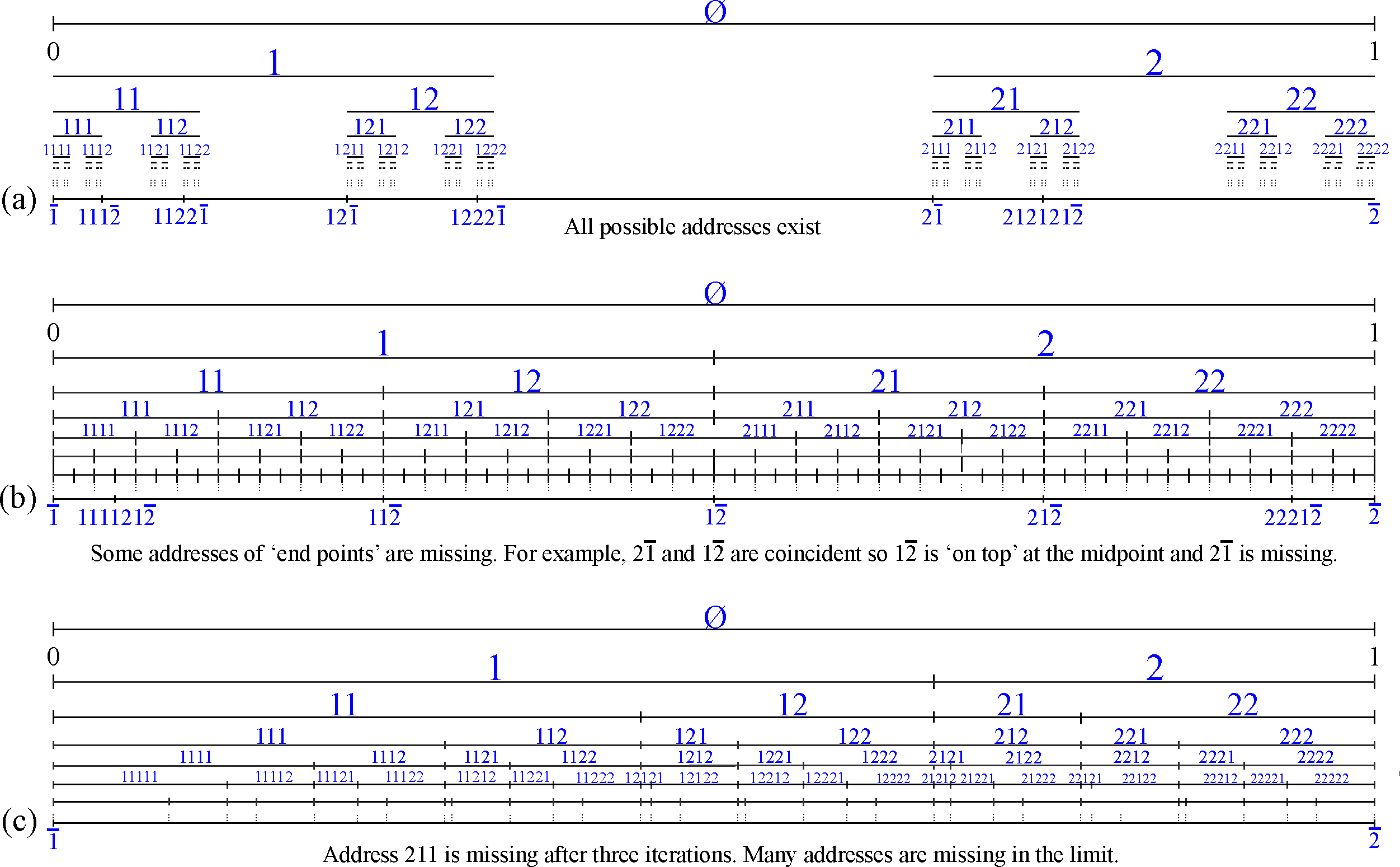
EXAMPLE 3 For the i.f.s. the strings and both belong to and are reversible. Figure 3 and Figure 4 illustrate two ways of looking at the development of top addresses. Figure 5 (a) illustrates the sets in for . We usually use lexicographic ordering to define top addresses, but Figure 4 uses standard ordering.

EXAMPLE 4 For the i.f.s. each of the strings belongs to and is reversible. Figure 5(b) illustrates the sets in for . Here it appears that all addresses are reversible.

Let us define a new tile to be a tile at level that is not contained in any tile at level Also, a child or child tile, is a tile at level that is contained in a tile, its parent at level
Theorem 5.2
Let be an invertible contractive i.f.s. on , as defined in Equation 3. Let be reversible. Each tile in is either (i) a nonempty subset, the child of a tile in of the form or (ii) a nonempty set of the form where a new tile. Each tile in contains exactly one child in .
Proof
We can write
Each tile in the first set is a subset of a tile in and it is non-empty because is reversible. (By reversibility, the set of top addresses is nonempty.)
Consider any tile in the second set. By Lemma 4: if then which is not possible because . So no tile in the second set is contained in a tile in the first set. That is to say, the tiles in the second set, which have non-cancelling addresses, are “new” and do not contain any tile in the first set.
This says that every tile at level has a unique child at level either equal to its parent, or smaller but not empty; also, there are new tiles at level which do not have predecessors at level , because Each tile in contains a child in . One deduces that is tiled by new tiles.
In the special case also considered by Strichartz in Theorem 4.2, we have:
Theorem 5.3
Let be an invertible contractive i.f.s. on , as defined in Equation 3. Then is a well defined tiling of specifically and
Each tile (for all ) in can be written for some for some with The tile corresponds to
Proof
The result follows from the observation that in this case all children are exact copies of their parents. To see this simply note that for all
For future work, one can consider the case where is homeomorphic to a ball. By introducing a stronger notion of reversibility (see also tilings ), that requires the tops dynamical system orbit of a reversible point to be contained in a compact set contained in the interior of one can ensure that new tiles are located further and further away from This means that new tiles have only finitely many successive generations of children (one child at each subsequent generation) before children are identical to their parents. Hence, given any ball of finite radius, the set of tiles in that have nonempty intersection with remains constant for all large enough In such cases one is constant for all sufficiently large, and so the tiling is well defined. We note that if is disjunctive then see tilings .
We conjecture that if is homeomorphic to a ball and if is both reversible and disjunctive (relative to the top), then is a well defined tiling of
5.3 A leafy example of a two-dimensional top tiling
For a two-dimensional affine transformation we write
where . We consider the i.f.s. defined by the two similitudes
| (4) |
The attractor, =leaf, illustrated in Figure 6, is made of two overlapping copies of itself. The copy illustrated in black is associated with The point with top address is represented by the tip of the stem of the leaf. The stem is actually arranged in an infinite spiral, not visible in the picture. In all tiling pictures, the colors of the tiles were obtained by overlaying the tiling on a colorful photograph: the color of each tile is the color of a point beneath it. In this way, if the tiles were very small, the tiling would look like a mozaic representation of the underlying picture.

Figure 7 illustrates the top of at depths labelled by the addresses in .

Figure 8 illustrates the successive blowups for for the i.f.s. in Equation (5.2). See also Figure 9 where the successive images are illustrated in their correct relative positions.


Figure 10 shows a patch of a leaf tiling, illustrating its complexity. Figure 11 illustrates a patch of a top tiling obtained using an i.f.s. of four maps.


ACKNOWLEDGEMENTS: We thank both Brendan Harding and Giorgio Mantica for careful reading and corrections.
References
- (1) C. Bandt, S.Graf, Self-similar sets VII. A characterization of self-similar fractals with positive Hausdorff measure, Proc. Amer. Math. Soc. 114 (1992), 995-1001.
- (2) C. Bandt, Self-similar tilings and patterns described by mappings, Mathematics of Aperiodic Order (ed. R. Moody) Proc. NATO Advanced Study Institute C489, Kluwer, (1997) 45-83.
- (3) C. Bandt, M. F. Barnsley, M. Hegland, A. Vince, Old wine in fractal bottles I: Orthogonal expansions on self-referential spaces via fractal transformations, Chaos, Solitons and Fractals, 91 (2016), 478-489.
- (4) M. F. Barnsley, A. Vince, Fractal tilings from iterated function systems, Discrete and Computational Geometry, 51 (2014), 729-752.
- (5) M. F. Barnsley, A. Vince, Self-similar polygonal tilings, Amer. Math. Monthly, 124 (2017), 905-921.
- (6) M. F. Barnsley, K. Leśniak, M. Rypka, Basic topological structure of fast basins, Fractals 26 (2018), no. 1, 1850011.
- (7) M. F. Barnsley, M. F., Theory and Applications of Fractal Tops, in: Levy-Vehel, J., Lutton, E., (eds.)Fractals in Engineering: New Trends in Theory and Applications. Springer, London (2005).
- (8) J. Hutchinson, Fractals and self-similarity, Indiana Univ. Math. J. 30 (1981), 713-747.
- (9) R. S. Strichartz, Fractals in the large, Canad. J. Math., 50 (1998), 638-657.
- (10) R. S. Strichartz, Differential Equations on Fractals, Princeton University Press, Princeton, New Jersey (2006).
- (11) A. Teplyaev, Spectral analysis on infinite Sierpinski gaskets, J. Funct. Anal. 129 (1998), 357-567.