Blowup for the defocusing septic complex-valued nonlinear wave equation in $\mathbb{R}^{4+1}$

Tristan Buckmaster Courant Institute of Mathematical Sciences, New York University, New York, NY 10012. [email protected] and Jiajie Chen Courant Institute of Mathematical Sciences, New York University, New York, NY 10012. [email protected]

Abstract.

In this paper, we prove blowup for the defocusing septic complex-valued nonlinear wave equation in $\mathbb{R}^{4+1}$ . This work builds on the earlier results of Shao, Wei, and Zhang [56, 55], reducing the order of the nonlinearity from $29$ to $7$ in $\mathbb{R}^{4+1}$ . As in [56, 55], the proof hinges on a connection between solutions to the nonlinear wave equation and the relativistic Euler equations via a front compression blowup mechanism. More specifically, the problem is reduced to constructing smooth, radially symmetric, self-similar imploding profiles for the relativistic Euler equations.

As with implosion for the compressible Euler equations, the relativistic analogue admits a countable family of smooth imploding profiles. The result in [56] represents the construction of the first profile in this family. In this paper, we construct a sequence of solutions corresponding to the higher-order profiles in the family. This allows us to saturate the inequalities necessary to show blowup for the defocusing complex-valued nonlinear wave equation with an integer order of nonlinearity and radial symmetry via this mechanism.

1. Introduction

We investigate finite time blowup for the complex-valued defocusing nonlinear wave equation:

(1.1)

\partial_{tt}w=\Delta w-|w|^{p-1}w,

for $w(t,x):\mathbb{R}\times\mathbb{R}^{d}\to\mathbb{C}$ . Given smooth and well-localized initial data $(w(0),\partial_{t}w(0))$ , the classical Cauchy theory states that (1.1) admits a smooth and strong local-in-time solution $w(t)$ [61]. The parameters $(d,p)$ , can be naturally classified in terms of the critically of the conserved energy

E(w(t))\triangleq\int_{\mathbb{R}^{d}}\frac{1}{2}(|\partial_{t}w|^{2}+|\nabla w|^{2})+\frac{1}{p+1}|w|^{p+1}dx,

in terms of the scaling symmetry

w(t,x)\to w_{\lambda}(t,x)\triangleq\lambda^{\frac{2}{p-1}}w(\lambda t,\lambda x),\quad\lambda>0.

Precisely, we obtain three regimes: the subcritical case, $d\leq 2$ or $p<1+\frac{4}{d-2}$ for $d\geq 3$ ; the critical case, $p=1+\frac{4}{d-2}$ and $d\geq 3$ ; and the supercritical case, $p>1+\frac{4}{d-2}$ and $d\geq 3$ .

The blowup of nonlinear wave equations has been extensively studied in the focusing case (cf. [3, 46, 38, 45, 24, 25, 26, 27, 37, 40, 41, 42, 43]). For the defocusing case, the equation is globally well-posed in the subcritical and critical case [28, 29, 32, 31, 57, 58, 39, 63]. Nevertheless, the question of blowup or global well-posedness for smooth solutions to defocusing nonlinear Schrödinger or wave equation has remained a long-standing open problem [65]. Tao, in [64], showed if one considers a supercritical, high dimensional, defocusing nonlinear wave system $\Box u=(\nabla_{\mathbb{R}^{m}}F)(u)$ , for some smooth, positive, carefully designed potential $F:\mathbb{R}^{m}\rightarrow\mathbb{R}$ , one proves blowup in finite time. Recently, in the breakthrough work of Merle, Raphael, Rodnianski and Szeftel [50], blowup for the supercritical defocusing nonlinear Schrödinger equation was proven via a novel front compression mechanism, whereby the phase of the solution blows up. The work [49] leverages a connection between the nonlinear Schrödinger equations and the compressible Euler equations with an added quantum pressure term via Madelung’s transformation. Under the appropriate scaling assumptions – which necessitates considering dimensions $\geq 5$ and high order nonlinearities – the quantum pressure term becomes lower order, which enabled the use of self-similar imploding profiles to the compressible Euler equations constructed in [51], as asymptotic self-similar profiles to the defocusing nonlinear Schrödinger equation.

Inspired by the work [50], Shao, Wei, and Zhang in [56, 55] recently exploited a similar front compression mechanism to establish blowup for the defocusing nonlinear wave equation (1.1) via a self-similar profile to the relativistic Euler equations. Specifically, they proved finite time blowup of (1.1) from smooth compactly supported initial data with dimension $d$ and odd nonlinearity $p$ satisfying $d=4,p\geq 29$ and $d\geq 5,p\geq 17$ . See also Theorem 1.2.

1.1. Self-similar ansatz

We consider the phase-amplitude representation $w=\rho e^{i\phi}$ with $\rho,\phi$ being real and rewrite (1.1) as the system of $(\rho,\phi)$ . To this end, we compute

	$\displaystyle\partial_{tt}w$	$\displaystyle=\Big{(}\partial_{tt}\rho+i\partial_{t}(\partial_{t}\phi\rho)+i\partial_{t}\phi(\partial_{t}\rho+i\partial_{t}\phi\rho)\Big{)}e^{i\phi},$
	$\displaystyle\Delta w$	$\displaystyle=(\Delta\rho+i\nabla\cdot(\rho\nabla\phi)+i\nabla\rho\cdot\nabla\phi-\rho\|\nabla\phi\|^{2})e^{i\phi}.$

Substituting the above computation into (1.1), dividing by $e^{i\phi}$ and then taking the real and imaginary part of the equation, we derive the equations for $\rho$ and $\phi$


(1.2a)	$\displaystyle\partial_{tt}\rho$	$\displaystyle=\rho\|\partial_{t}\phi\|^{2}+\Delta\rho-\rho\|\nabla\phi\|^{2}-\|\rho\|^{p-1}\rho,$
(1.2b)	$\displaystyle\partial_{tt}\phi\cdot\rho$	$\displaystyle=-2\partial_{t}\phi\partial_{t}\rho+\rho\Delta\phi+2\nabla\rho\cdot\nabla\phi.$

We consider the general self-similar blowup ansatz

(1.3)

\rho=\frac{1}{(T-t)^{a}}W(\frac{x}{(T-t)^{c}}),\quad\phi=\frac{1}{(T-t)^{b}}\Phi(\frac{x}{(T-t)^{c}}),

for some $a,b,c$ to be determined.

In line with front compression, where the phase $\phi$ blows up, we consider $b>0$ for our self-similar ansatz (1.3). Moreover, to obtain a collapsing blowup, which is natural due to the conservation of the energy, we impose $c>0$ . We use the notation $A\asymp B$ to denote that $A$ and $B$ are comparable up to a $t-$ independent constant. Under these assumptions, for $T-t\ll 1$ , we get

(1.4)

\begin{gathered}\partial_{tt}\rho\asymp(T-t)^{-a-2},\ \Delta\rho\asymp(T-t)^{-a-2c},\\ \rho|\partial_{t}\phi|^{2}\asymp(T-t)^{-a-2-2b},\quad\rho|\nabla\phi|^{2}\asymp(T-t)^{-a-2b-2c},\quad|\rho|^{p-1}\rho\asymp(T-t)^{-pa}.\end{gathered}

Since $b>0$ , we treat $\partial_{tt}\rho,\Delta\rho$ in (1.2a) as lower order terms. For the $\phi$ -equation (1.2b), it is easy to observe that the scalings of each terms are balanced. Thus, dropping $\partial_{tt}\rho,\Delta\rho$ in (1.2a) and then dividing $\rho$ on both sides of (1.2a), we derive the following leading order system of (1.2a)

(1.5)

|\partial_{t}\phi|^{2}-|\nabla\phi|^{2}=|\rho|^{p-1}.

To balance these three terms, using (1.4), we impose the following relation among $a,b,c$ in (1.3)

(1.6)

c=1,\quad(p-1)a=2(b+1),\quad b>0.

Note that equations (1.5) and (1.2b) reduce to isentropic relativistic Euler equation. In fact, by introducing $\ell=\frac{4}{p-1}+1$ , the flat Lorentz metric $g=(g^{\mu\nu})$ and derivative $\partial^{\mu}$ as

g^{00}=-1,\quad g^{\mu\nu}=\delta_{\mu\nu},\quad\forall(\mu,\nu)\neq(0,0),\quad\partial^{\mu}=g^{\mu\nu}\partial_{\nu},

the relativistic velocity $\mathbf{u}=(u^{0},u^{1},..,u^{d})$ , the energy density $\varrho$ , the energy momentum tensor $T^{\mu\nu}$ , and the pressure $P$ subject to the isothermal equation of state as follows

(1.7a)		$\varrho=\rho^{p+1},\quad u^{0}=\rho^{-\frac{p-1}{2}}\partial_{t}\phi,\quad u^{i}=\rho^{-\frac{p-1}{2}}\partial^{i}\phi,\quad T^{\mu\nu}=(P+\varrho)u^{\mu}u^{\nu}+Pg^{\mu\nu},$
we derive the relativistic Euler equations
(1.7b)		$u^{\mu}\partial_{\mu}\varrho+(P+\varrho)\partial_{\mu}u^{\mu}=0,\quad\partial_{\mu}T^{\mu\nu}=0,\quad P=\frac{1}{\ell}\varrho,$

with normalization $\|\mathbf{u}\|_{g}^{2}=g_{\mu\nu}u^{\mu}u^{\nu}=-1$ . The above connection between the defocusing wave equations and the relativistic Euler equations has been used in [56].

The local existence of smooth solutions to the relativistic Euler equations was established in [48], with some global existence results in [60, 54, 14]. Meanwhile, the equations can develop a finite time singularity [35, 53, 21]. For more discussions on the mathematical aspects of relativistic fluids, see the surveys [23, 2].

1.2. Main results

By imposing the radial symmetry on $\rho,\phi$ and plugging the self-similar ansatz (1.3) in equations (1.2b) and (1.5), we can derive the ODE (2.3) for the self-similar profiles $W,\Phi$ (1.3). See the derivation in Section 2.1.

To use the front compression mechanism for smooth blowup, we require $(d,p)$ to satisfy

(1.8)

\ell+\ell^{1/2}<d-1,\quad\ell=1+\frac{4}{p-1}>1,

which implies $d\geq 4$ and the non-linear exponent $p\geq p(d)$ . For $d=4$ and integer $p$ , this implies $p\geq 7$ . See Section 2.1 for more details about these constraints. In this paper, we consider the lowest dimension $d=4$ in this setting and the smallest integer exponent $p=7$ in this dimension.

Our main result is stated as follows.

Theorem 1.1.

Let $d=4,p=7,\ell=\frac{4}{p-1}+1$ , and $n$ be an odd number and large enough. There exists $\gamma_{n}$ accumulating at $\ell^{-1/2}$ with $\gamma_{n}>\ell^{-1/2},b_{n}=\frac{d-1}{\ell(\gamma_{n}+1)}-1>0$ such that the ODE (2.3) admits a smooth solution $V^{(\gamma_{n})}\in C^{\infty}[0,\infty)$ with $V^{(\gamma_{n})}(0)=0$ ,

(1.9)

V^{(\gamma_{n})}(Z)\in(-1,1),\quad V^{(\gamma_{n})}(Z)<Z,

for any $Z>0$ , and $V(Z)=Z\tilde{V}(Z^{2})$ for some function $\tilde{V}\in C^{\infty}[0,\infty)$ . Moreover, the solution gives rise to a smooth radially symmetric self-similar profile $(W,\Phi)$ in (1.3) and a solution to the relativistic Euler equations (1.2b) and (1.5) on $[0,T)\times\mathbb{R}^{d}$ :

(1.10)

u^{0}(t,x)=U^{0}(Z),\quad u^{i}(t,x)=U(Z)\frac{x_{i}}{r},\quad\varrho(t,x)=(T-t)^{-\frac{(d-1)(\ell+1)}{\ell(\gamma+1)}}W^{p+1}(Z),

where $r=|x|,Z=\frac{r}{T-t}$ . The solution develops an imploding singularity at $t=T,x=0$ and satisfies the asymptotics

(1.11)

\lim_{Z\to\infty}U^{0}(Z)=U^{0}_{\infty},\quad\lim_{Z\to\infty}U(Z)=U_{\infty},\quad\lim_{Z\to\infty}\varrho(t,x)=\varrho_{\infty}|x|^{-\frac{(d-1)(\ell+1)}{\ell(\gamma+1)}}

for any $x\neq 0$ and some constants $U^{0}_{\infty}\neq 0,U_{\infty},\varrho_{\infty}>0$

To further prove blowup of the nonlinear wave equation (1.1), we use [55, Theorem 1.1]:

Theorem 1.2 (Theorem 1.1 [55]).

Let $d\in\mathbb{Z}\cap[4,\infty),p\in 2\mathbb{Z}_{+}+1,\ell=\frac{4}{p-1}+1$ with $d-1>\ell+\ell^{1/2}$ . Suppose that there exists $\gamma$ with $\gamma>\ell^{-1/2}$ and $(d-1)>\ell(\gamma+1)$ ¹¹1 The parameter $\beta,k$ in [55] corresponds to $\beta=1+b=\frac{d-1}{\ell(\gamma+1)}$ (1.3), (2.1) and $k=d-1$ in this paper. The condition $\beta\in(1,k/(\ell+\ell^{1/2}))$ in [55, Theorem 1] is equivalent to $\gamma>\ell^{-1/2}$ and $d-1>\ell(\gamma+1)$ (2.4). such that the ODE (2.3) with parameters $(d,p,\gamma)$ admits a smooth solution $V(Z)$ defined in $Z\in[0,\infty)$ satisfying $V(Z)\in(-1,1),V(0)=0$ and $V(Z)=Z\tilde{V}(Z^{2})$ for some function $\tilde{V}\in C^{\infty}[0,\infty)$ .

Then there exists smooth compactly supported functions $w_{0},w_{1}:\mathbb{R}^{d}\to\mathbb{C}$ such that the defocusing nonlinear wave equation (1.1) with nonlinearity $p$ develops a finite time singularity from the initial data $w(0)=w_{0},\partial_{t}w(0)=w_{1}$ .

In Theorem 1.1, since $\gamma_{n}>\ell^{-1/2}$ and $\gamma_{n}$ converges to $\ell^{-1/2}$ as $n\to\infty$ , for $n$ large enough, the parameters $(d=4,p=7,\gamma_{n})$ satisfies the inequalities in Theorem 1.2. Moreover, the smooth solution $V^{(\gamma_{n})}$ constructed in Theorem 1.1 satisfies the assumptions in Theorem 1.2. Thus, using Theorems 1.1 and 1.2, we establish:

Corollary 1.3.

There exists smooth compactly supported functions $w_{0},w_{1}:\mathbb{R}^{4}\to\mathbb{C}$ such that the septic defocusing nonlinear wave equation (1.1) with $p=7$ develops a finite time singularity from the initial data $w(0)=w_{0},\partial_{t}w(0)=w_{1}$ .

Remark 1.4.

In dimension $d=4$ with nonlinearity $p\in 2\mathbb{N}+1$ , the range of parameter in the supercritical case $p>1+\frac{4}{d-2}$ implies that $p\geq 5$ and $p\in 2\mathbb{N}+1$ . Our result resolves the case $p=7$ . It is conceivable that our methods for proving Theorem 1.1 can apply to a specific pair of parameters $(d,p)$ with $p\in 2\mathbb{N}+1$ , provided they satisfy (1.8). Note that the parameters $(d,p)$ in the supercritical case $p>1+\frac{4}{p-2}$ with $d\geq 4$ and $p\in 2\mathbb{N}+1$ that do not satisfy (1.8) are $(d,p)=(4,5),(5,3)$ .

Similar to the results in [55], we only construct blowup for (1.1) with a complex-valued solution. Blowup of (1.1) with real-valued solution remains open.

The main difficulty to prove Theorem 1.1 is that the ODE (2.3) of $(Z,V)$ is singular near a sonic point. Additionally, the ODE degenerates near the sonic point as $\gamma\to\ell^{-1/2}$ . We remark that, due to the constraint (1.8), constructing the blowup solution to (1.1) with smaller $p$ requires considering $\gamma$ close to $\ell^{-1/2}$ . To overcome these difficulties, we renormalize the ODE (2.3) to obtain a new ODE of $(Y,U)$ (2.14), which is non-degenerate near the sonic point as $\gamma\to\ell^{-1/2}$ . To analyze the $(Y,U)$ -ODE near the sonic point, we perform power series expansion of $U(Y)$ and estimate the asymptotics of the power series coefficients $U_{n}$ using induction. Using barrier arguments, a shooting argument, and a few monotone properties, we extend the local power series solution to a global solution of the ODE.

The proof involves light computer assistance, mainly to derive the power series coefficients $U_{i}$ for $i\leq 500$ and to verify the signs of a few lower-order polynomials. These calculations can be performed on a personal laptop in a few seconds. See more details in Appendix B.

We will derive the ODE (2.3) and its renormalization (2.14) and analyze its basic properties in Section 2. We outline the proof and the organization of Sections 3-6 in Section 2.5.

1.3. Comparison with the methods in existing works

Our proof share some similarities with [6], including some barrier arguments, estimates of the power series coefficients using induction, and computer-assisted proofs. Different from [6], we need to renormalize the ODE to overcome the degeneracy as $\gamma\to\ell^{-1/2}$ .

In [6], the estimates of the asymptotics of power series coefficients $U_{n}$ involve ad-hoc partitions of $n$ . We develop a systematic approach for the estimates by identifying a few leading order terms in the recursive formula of $U_{n}$ and treating the remaining terms perturbatively. We check a few properties of $U_{i},i=1,2,..,N$ for $N$ suitably large with computer assistance and then perform induction for the remaining coefficients. This allows us to impose a stronger induction hypothesis, resulting in a streamlined approach to estimating the higher order coefficients, which further leads to a simplified splitting in $n$ . Moreover, our scheme of estimates does not utilize special forms of the ODE and are readily generalized to ODE (2.3) or (2.14) with numerator and denominator being higher order polynomials. Additional simplifications of the combinatorial estimates are made via renormalization of the power series coefficients. See Section 3.

We follow the connection between the defocusing nonlinear wave equation and the relativistic Euler equation used in [56] to derive the ODE (2.3) governing the profiles, use the same renormalization as in [56], and adopt a few basic derivations for the ODEs from [56]. However, there are a few key differences. Firstly, we apply renormalization to overcome the degeneracy of the ODE as $\gamma\to\ell^{-1/2}$ , whereas in [56], renormalization is used to simplify computations and obtain blowup results for a wider range of $(d,p)$ . We can also employ other renormalization to overcome this degeneracy; see Remark 2.3. We adopt the renormalization from [56] to simplify certain presentations and derivations that are less essential. Secondly, since we consider a smaller nonlinearity ( $p=7$ ) than those considered in [56], we need to use much higher-order barrier functions near the sonic point than those in [56], which are based on quartic or lower-order polynomials. Thirdly, by taking $\gamma\to\ell^{-1/2}$ , we obtain a large parameter $\kappa(\gamma)$ (2.30) and use it and light computer assistance to bypass several detailed computations in [56].

We note that in [34], Guo, Hadzic, Jang, and Schrecker employed similar arguments, such as Taylor expansions, dynamical systems analysis, and computer-assisted proofs, to construct smooth self-similar solutions for the gravitational Euler-Poisson system.

1.4. Related results

In this section, we review related results on singularity formation and computer-assisted proofs in fluid mechanics

Smooth Implosions

The construction of the self-similar imploding singularity in Theorem 1.1 is closely related to that in compressible fluids. Guderley [33] was the first to construct radial, non-smooth, imploding self-similar singularities along with converging shock waves in compressible fluids. While Guderley’s setting has been extensively studied, the existence of a finite-time smooth, radially symmetric implosion (without shock waves) was only recently established in [51, 52, 50]. Subsequently, radially symmetric implosion in $\mathbb{R}^{3}$ with a larger range of adiabatic exponents was established in [6], and non-radial implosion was established in [12, 11]. While these results are inspired by Guderley’s setting, constructing $C^{\infty}$ self-similar implosion profiles is challenging due to the degeneracy at the sonic point, requiring sophisticated mathematical techniques [51] or computer-assisted methods [6]. The smooth imploding solutions are proved to be potentially highly unstable [52, 6, 12, 50], with numerical studies of instabilities presented in [5]. The self-similar profile in Guderley’s setting was recently constructed in [36]. By perturbing the radial implosion [51], exploiting axisymmetry, and proving the full stability of the perturbation generated by angular velocity, vorticity blowup in the compressible Euler equations was established in [16] for the case of $\mathbb{R}^{2}$ and in [15] for $\mathbb{R}^{d}$ with $d\geq 3$ .

Shock formation

The prototypical singularity for the compressible Euler equations is the development of a shock wave. Rigorous work regarding shocks traces back to the work of Lax [44]. Shock wave singularities in the multi-dimensional, irrotational, isentropic setting was first analyzed by Christodoulou in the work [21] (cf. [22]). This work was later extended to include non-trivial vorticity in the 2-dimensional setting by Luk and Speck [47]. Restricting to 2-dimensions and assuming azimuthial-symmetry, the first complete description of the formation of a shock singularity, including its self-similar structure was given in a work of the first author, Shkoller, and Vicol [8]. This latter work was extended by the authors to 3-dimensions in the absence of symmetry assumptions in [9] and to the 3-dimensional non-isentropic setting in [10]. Returning to the setting of 2-dimensions under azimuthial-symmetry, the first full description of shock development past the first singularity was proven in a work by the first author, Drivas, Shkoller, and Vicol [7]. Shock development in the absence of symmetry remains an open problem; however, recently Shkoller, and Vicol in the work [59] constructed compact in time maximal development in the 2-dimensional setting, which is a crucial step towards resolving this major open problem (partial results in direction of maximal development were earlier attained in [1]).

Computer-assisted proofs in fluids

In recent years, there have been substantial developments in computer-assisted proofs in mathematical fluid mechanics. We highlight a few advancements in incompressible fluids: singularity formation in the 3D Euler equations [18, 17] and related models [19, 20], constructing nontrivial global smooth solutions to SQG [13], and some applications to Navier-Stokes [4, 66]. See also the survey [30].

2. Autonomous ODE for the self-similar profile

In this section, we derive the ODE governing the self-similar profile (1.3) and perform renormalization to overcome some degeneracy.

2.1. ODE for the profile

We introduce $\ell=\ell(p)$ and a free parameter $\gamma$ to rewrite $(a,b)$ in (1.3), (1.6) as follows

(2.1)

\ell=\frac{4}{p-1}+1,\quad b=\frac{d-1}{\ell(\gamma+1)}-1,\quad a=\frac{2(d-1)}{(p-1)\ell(\gamma+1)}.

where $d$ is the dimension. We impose radial symmetry on the solution $(\rho,\phi)$ . As a result, the profiles $W,\Phi$ in (1.6) are radially symmetric. We introduce the radial and self-similar variables

(2.2a)		$r=\|x\|,\quad z=\frac{x}{T-t},\quad Z=\|z\|=\frac{\|x\|}{T-t}.$
From the ansatz (1.3) and (1.6), it is easy to see that $\rho^{-\frac{p-1}{2}}\partial_{t}\phi(x,t),\rho^{-\frac{p-1}{2}}\partial_{r}\phi(x,t)$ only depend on $Z$ . Thus, to solve (1.5), we consider
(2.2b)		$\rho^{-\frac{p-1}{2}}\partial_{t}\phi(x,t)=\frac{1}{(1-V(Z)^{2})^{1/2}},\quad\rho^{-\frac{p-1}{2}}(\partial_{r}\phi)(x,t)=\frac{V(Z)}{(1-V(Z)^{2})^{1/2}}.$

The relation (2.2) and (1.2b) imply that $V(Z)$ solves the following ODE for $Z\geq 0$

(2.3)	$\displaystyle\frac{dV}{dZ}$	$\displaystyle=\frac{\Delta_{V}(Z,V)}{\Delta_{Z}(Z,V)},$
	$\displaystyle\Delta_{V}$	$\displaystyle=(d-1)(1-V^{2})\Big{(}\frac{1}{\gamma+1}(1-V^{2})Z-V(1-VZ)\Big{)},$
	$\displaystyle\Delta_{Z}$	$\displaystyle=Z((1-ZV)^{2}-\ell(V-Z)^{2}).$

This ODE was first derived in [56]. For completeness, we derive the ODE in Appendix A.1. ²²2 We have substitute $k=d-1,m=\frac{d-1}{1+\gamma}$ in the ODEs derived in [56, Section 2] to reduce the number of variables. Moreover, we have used $\beta=\frac{(d-1)(\ell+1)}{\ell(\gamma+1)}$ to remove the parameter $\beta$ used in [56]. Note that the meaning of $\beta$ is different in [56] and [55].

Constraints on the parameters

From $b>0$ (1.6), which is related to the front compression mechanism and the relation (2.1), we first require $\gamma$ to satisfy

(2.4)

\frac{d-1}{\ell(\gamma+1)}>1\iff d-1>\ell(\gamma+1).

To obtain a smooth ODE solution, we have an additional constraint on $\gamma$ established in [56, Lemma 2.1].

Lemma 2.1 (Lemma 2.1 [56]).

If $V(Z):[0,1]\to(-1,1)$ is a $C^{1}$ solution to (2.3) with $V(0)=0$ and $\ell>1,\gamma>-1,d>1$ , then $\gamma>\ell^{-1/2}$ .³³3 In [56, Lemma 2.1], the assumptions $m>0,k>0$ are equivalent to $\gamma>-1,d>1$ in our notations due to the relation $m=\frac{k}{\gamma+1},k=d-1$ . [56, Lemma 2.1] implies that $k>m(1+\ell^{-1/2})$ , which is equivalent to $\gamma>\ell^{-1/2}$ . Again, we do not use the parameters $k,m$ as [56] to reduce the number of variables.

Combining (2.4) and the lower bound $\gamma>\ell^{-1/2}$ from the Lemma 2.1, we obtain

(2.5)

\quad\ell+\ell^{1/2}<d-1,\quad\ell<\ell_{u}(d):=(\sqrt{d-\frac{3}{4}}-\frac{1}{2})^{2}.

Since $\ell>1$ , we need $d\geq 4$ . Recall the power of non-linearity $p=\frac{4}{\ell-1}+1,\ell(p)=1+\frac{4}{p-1}$ (2.1). Let $p(d)$ be the value with $\ell(p(d))=\ell_{u}(d)$ . For $d=4,5,6$ , the constraint (2.5) implies

p>p(d),\quad p(4)\approx 6.737,\quad p(5)\approx 3.7808,\quad p(6)\approx 2.8110.

In the remainder of the paper, we will focus on the lowest dimension $d=4$ and the smallest integer power $p=7$ in this dimension. Then, we have

(2.6)

d=4,\quad p=7,\quad\ell=\frac{5}{3}.

We still have one free parameter $\gamma$ , which will be chosen so that $0<\gamma-\ell^{-1/2}\ll 1$ .

Double roots and the sonic point

Solving $\Delta_{V}(P)=\Delta_{Z}(P)=0$ , we get the special points

(2.7)

\begin{gathered}P_{O}=(0,0),\quad P_{s}=(Z_{0},V_{0})=\Big{(}\tfrac{(\gamma+1)\sqrt{\ell}}{\ell\gamma+1},\tfrac{1}{\gamma\sqrt{\ell}}\Big{)},\quad P_{2}=(1,1),\quad P_{3}=(0,1),\end{gathered}

where $P_{s}$ is the sonic point. The letters $O,s$ are short for origin, sonic, respectively.

The smoothness of the ODE solution to (2.3) is closely related to the Jacobian of a renormalization of the ODE (2.3) by the factor $\Delta_{Z}$ :

(2.8)

M_{P}:=\begin{pmatrix}\partial_{V}\Delta_{V}&\partial_{Z}\Delta_{V}\\ \partial_{V}\Delta_{Z}&\partial_{Z}\Delta_{Z}\\ \end{pmatrix}.

A direct computation shows that the entries degenerate: $|M_{P,ij}|\lesssim|\gamma^{2}\ell-1|$ , as $\gamma\to\gamma_{*}=\ell^{-1/2}$ , which complicates the analysis of the ODE near the sonic point.

Notations and parameters

Throughout the paper, we will use $(Z,V)$ for the variables in the original ODE system (2.3), and $(Y,U)$ for the renormalized ODE (2.14) to be introduced. We further introduce some parameters

(2.9)

\displaystyle\varepsilon=\ell\gamma^{2}-1,\quad A=d+1-(d-1-2\ell)\gamma,\quad B=2d-1-\ell,

and will use them to denote the coefficients of a polynomial in the renormalized ODE of $(U,Y)$ .

We fix the following constants

(2.10)

\hat{\delta}=0.049,\quad\delta=0.05,

and will use them to denote the size of relative error for asymptotic series around the sonic point (see Lemma 3.5 and Corollary 3.11).

We denote $A\lesssim B$ if $A\leq CB$ for some absolute constant $C>0$ , and denote $A\asymp B$ if $A\lesssim B$ and $B\lesssim A$ . We denote $A\lesssim_{m}B$ if $A\leq C(m)B$ for some constant $C(m)>0$ depending on $m$ , and define the notations $A\asymp_{m}B$ similarly.

2.2. Renormalization

To overcome the degeneracy of the Jacobian $M_{P}$ (2.8) as $\gamma\to\gamma_{*}$ , we study an ODE system equivalent to (2.3) by performing a renormalization of the system. We adopt the change of coordinate $(Z,V)\to(Y,U)=({\mathcal{Y}},{\mathcal{U}})(Z,V)$ from [56] with

(2.11)

\displaystyle{\mathcal{Y}}(Z,V)=\frac{(1-V^{2})Z-(\gamma+1)V(1-VZ)}{Z(1-V^{2})},\quad{\mathcal{U}}(Z,V)=\frac{(\gamma+1)^{2}(1-VZ)^{2}}{(1-V^{2})Z^{2}}.

We will see later that the Jacobian of the new ODE system in $(Y,U)$ at the sonic point (2.26) is non-degenerate as $\gamma\to\gamma_{*}$ . There are a few other change of coordinates that achieve this purpose. See Remark 2.3. The above transform (2.11) leads to lower order polynomials $\Delta_{U},\Delta_{Y}$ in $U$ , which simplifies some analysis. Note that we do not use this property in an essential way.

We can invert the transform from $(Y,U)$ to $(Z,V)=({\mathcal{Z}},{\mathcal{V}})(Y,U)$ using the following formulas

(2.12)

{\mathcal{Z}}(Y,U)=\frac{\sqrt{U+(1-Y)^{2}}}{\frac{1}{1+\gamma}U+1-Y},\quad{\mathcal{V}}(Y,U)=\frac{1-Y}{\sqrt{U+(1-Y)^{2}}}.

The bijective properties are proved in [56, Lemma 3.8] :

Lemma 2.2.

Denote ${\mathcal{R}}_{ZV}=\{(Z,V):0<V<1,0<ZV<1\},{\mathcal{R}}_{YU}=\{(Y,U):U>0,Y<1\}$ . Then $({\mathcal{Y}},{\mathcal{U}}):{\mathcal{R}}_{ZV}\to{\mathcal{R}}_{YU}$ is a bijection.

A direct computation yields that the inversion of $({\mathcal{Y}},{\mathcal{U}})$ is given by $({\mathcal{Z}},{\mathcal{V}})$ . Thus, for $(Z,V)\in{\mathcal{R}}_{ZV}$ or $(Y,U)\in{\mathcal{R}}_{YU}$ , we have

(2.13)

({\mathcal{Y}},{\mathcal{U}})\circ({\mathcal{Z}},{\mathcal{V}})=\mathrm{Id},\quad({\mathcal{Z}},{\mathcal{V}})\circ({\mathcal{Y}},{\mathcal{U}})=\mathrm{Id}.

Suppose that $(Z,V(Z))$ solves (2.3). We have the following ODE for $(Y,U)=({\mathcal{Y}},{\mathcal{U}})(Z,V(Z))$ :

(2.14)	$\displaystyle\frac{dU}{dY}$	$\displaystyle=\frac{\Delta_{U}(Y,U)}{\Delta_{Y}(Y,U)},$
	$\displaystyle\Delta_{U}$	$\displaystyle=2U(U+f(Y)+(d-1)Y(1-Y)),$
	$\displaystyle\Delta_{Y}$	$\displaystyle=(dY-1)U+(Y-1)f(Y),\quad f(Y)=-\varepsilon-AY+BY^{2},$

where $\varepsilon,A,B$ are defined in (2.9). We refer to [56, Section 3.2] for the derivations of (2.14).

Denote by $d_{U},d_{Y}$ the degree of $\Delta_{U},\Delta_{Y}$ as a polynomial in $U$ , respectively. We have

(2.15a)		$d_{U}=2,\quad d_{Y}=1.$
We can expand $\Delta_{U},\Delta_{Y}$ as polynomials in $U$
(2.15b)		$\Delta_{U}=\sum_{i\leq d_{U}}F_{i}(Y)U^{i},\quad\Delta_{Y}=\sum_{i\leq d_{Y}}G_{i}(Y)U^{i},$
where $F_{i},G_{i}$ are polynomials in $Y$ . We further define the maximum degree of these polynomials in $Y$ as follows
(2.15c)		$d_{F}=\max_{i}\deg F_{i}(Y),\quad d_{G}=\max_{i}\deg G_{i}(Y).$

For the above ODE system (2.14), we have

(2.15d)

d_{F}=2,\quad d_{G}=3.

In this new coordinate system $(Y,U)$ , the points $P_{O},P_{s}$ defined in (2.7) map to

(2.16)

Q_{O}=(Y=Y_{O},U=\infty),\quad Q_{s}=(Y_{0},U_{0}),\quad Y_{O}=\frac{1}{d},\quad Y_{0}=0,\quad U_{0}=\varepsilon.

Remark 2.3.

One can choose other change of variables to make the matrix $M_{P}$ (2.8) nonsingular and analyze the ODE in the new system. One candidate is the following simpler transform

{\mathcal{U}}(Z,V)=\frac{1-VZ}{1-V^{2}},\quad{\mathcal{Y}}(Z,V)=\frac{V-Z}{1-V^{2}}.

In the new system, the gradient at the sonic point does not degenerate in the limit $\gamma\to\gamma_{*}$

|\nabla_{U,Y}\Delta_{U}|\asymp 1,\quad|\nabla_{U,Y}\Delta_{Y}|\asymp 1.

The reason is that the transformation from $(Z,V)$ to $(Y,U)$ is singular near $P_{s}$ as $\gamma\to\gamma_{*}$ with $|\nabla_{Z,V}({\mathcal{U}},{\mathcal{Y}})|_{P_{s}}\sim(\gamma-\gamma_{*})^{-1}$ , which compensates the degeneracy: $|\nabla\Delta_{Z}|,|\nabla\Delta_{v}|\asymp\gamma-\gamma_{*}$ .

2.2.1. Change of coordinates

Recall the maps ${\mathcal{Z}},{\mathcal{V}}$ from $(Y,U)$ to $(Z,V)$ (2.11) and $({\mathcal{Y}},{\mathcal{U}})$ from $(Z,V)$ to $(Y,U)$ (2.12). Denote by ${\mathcal{M}}_{1},{\mathcal{M}}_{2}$ the Jacobians

(2.17)

{\mathcal{M}}_{1}(Y,U)=\begin{pmatrix}\partial_{Y}{\mathcal{Z}}&\partial_{U}{\mathcal{Z}}\\ \partial_{Y}{\mathcal{V}}&\partial_{U}{\mathcal{V}}\\ \end{pmatrix}(Y,U),\quad{\mathcal{M}}_{2}(Z,V)=\begin{pmatrix}\partial_{Z}{\mathcal{Y}}&\partial_{V}{\mathcal{Y}}\\ \partial_{Z}{\mathcal{U}}&\partial_{V}{\mathcal{U}}\\ \end{pmatrix}(Z,V).

For $(Z,V)\in{\mathcal{R}}_{ZV},(Y,U)\in{\mathcal{R}}_{YU}$ with ${\mathcal{R}}_{ZV},{\mathcal{R}}_{YU}$ defined in Lemma 2.2, the denominators in the maps (2.11), (2.12) do not vanish. Thus, the matrices ${\mathcal{M}}_{1},{\mathcal{M}}_{2}$ are not singular. Using (2.13), we have

(2.18)

{\mathcal{M}}_{1}((Y,U){\mathcal{M}}_{2}(Z,V)=\mathrm{Id},\quad\mathrm{for}\quad(Y,U)=({\mathcal{Y}},{\mathcal{U}})(Z,V).

Since $M_{i}$ is not singular, we get $\det({\mathcal{M}}_{i})\neq 0$ .

Along the ODE solution curve $(Y,U(Y))$ or $(Z,V(Z))$ , the ODE (2.14) and the above change of coordinates implies

\frac{\Delta_{U}}{\Delta_{Y}}=\frac{dU}{dY}=\frac{\frac{d{\mathcal{U}}(Z,V(Z))}{dZ}}{\frac{d{\mathcal{Y}}(Z,V(Z))}{dZ}}=\frac{{\mathcal{M}}_{2,21}+{\mathcal{M}}_{2,22}\frac{\Delta_{V}}{\Delta_{Z}}}{{\mathcal{M}}_{2,11}+{\mathcal{M}}_{2,12}\frac{\Delta_{V}}{\Delta_{Z}}}=\frac{{\mathcal{M}}_{2,21}\Delta_{Z}+{\mathcal{M}}_{2,22}\Delta_{V}}{{\mathcal{M}}_{2,11}\Delta_{Z}+{\mathcal{M}}_{2,12}\Delta_{V}},

where $Q_{ij}$ denotes the $ij$ -th component of a matrix $Q$ . Thus, there exists some continuous function $m(Y,U)$ such that

(2.19)

{\mathcal{M}}_{2}\cdot\begin{pmatrix}\Delta_{Z}\\ \Delta_{V}\\ \end{pmatrix}=m(Y,U)\begin{pmatrix}\Delta_{Y}\\ \Delta_{U}\\ \end{pmatrix},\quad{\mathcal{M}}_{1}\cdot\begin{pmatrix}\Delta_{Y}\\ \Delta_{U}\\ \end{pmatrix}=m^{-1}\begin{pmatrix}\Delta_{Z}\\ \Delta_{V}\\ \end{pmatrix},\quad m\neq 0,

for $(Z,V)=({\mathcal{Z}},{\mathcal{V}})(Y,U)\in{\mathcal{R}}_{ZV}\backslash P_{s}$ or equivalently $(Y,U)\in{\mathcal{R}}_{YU}\backslash Q_{s}$ . For $(Y,U)\in{\mathcal{R}}_{YU}\backslash Q_{s}$ , since $\det({\mathcal{M}}_{2})\neq 0$ and $(\Delta_{Z},\Delta_{V})\neq(0,0)$ , we obtain $m(Y,U)\neq 0$ .

2.3. Roots of $\Delta_{Z},\Delta_{V},\Delta_{Y},\Delta_{U}$

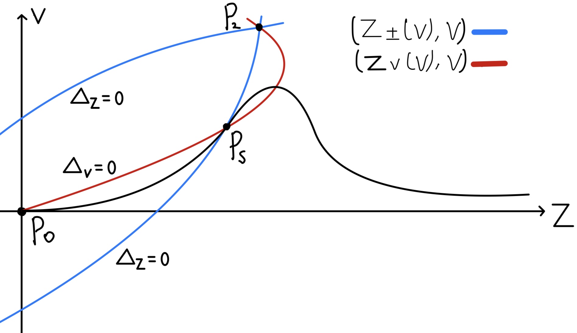
We can decompose $\Delta_{V},\Delta_{Z}$ , defined in (2.3) as follows

(2.20)		$\displaystyle\Delta_{V}$	$\displaystyle=\frac{d-1}{\gamma+1}(1-V^{2})(1+\gamma V^{2})(Z-Z_{V}(V)),\quad Z_{V}(V)=\frac{(1+\gamma)V}{1+\gamma V^{2}},$
(2.20)		$\displaystyle\Delta_{Z}$	$\displaystyle=Z(V^{2}-\ell)(Z-Z_{\pm}(V)),\quad Z_{\pm}(V)=\frac{\pm\ell^{1/2}V+1}{V\pm\ell^{1/2}}.$

The derivations follow from a direct computation. See Figure 1 for an illustration of the curves $Z_{V}(V)$ (red) and $Z_{\pm}(V)$ (blue). For $\gamma<1<\ell,|V|<1$ , a direct computation yields

(2.21)

\begin{gathered}Z_{V}^{\prime}(V)=(1+\gamma)\frac{1+\gamma V^{2}-2\gamma V^{2}}{(1+\gamma V^{2})^{2}}>0,\quad Z_{\pm}^{\prime}(V)=\frac{\ell-1}{(V\pm\ell^{1/2})^{2}}>0,\\ \quad Z_{+}(V)-Z_{-}(V)=\frac{2\ell^{1/2}(V^{2}-1)}{V^{2}-\ell}>0.\end{gathered}

Refer to caption — Figure 1. Illustrations of phase portrait of the $(Z,V)$ -ODE (2.3). The solution curve is in black and $Z_{\pm}(V),Z_{V}(V)$ defined in (2.20) are roots of $\Delta_{Z},\Delta_{V}$ .

Plugging the formulas of $Z,V$ (2.12) in $\Delta_{Z}$ (2.3) with $(Y,U)=({\mathcal{Y}},{\mathcal{U}})(Z,V)$ , we can also rewrite $\Delta_{Z}$ as

(2.22)

\Delta_{Z}=Z((1-ZV)^{2}-\ell(V-Z)^{2})=\frac{ZU^{2}(U+(1-Y)^{2}-\ell(Y+\gamma)^{2})}{(U+(1-Y)^{2})(U+(1+\gamma)(1-Y))^{2}}\Big{|}_{(Y,U)=({\mathcal{Y}},{\mathcal{U}})(Z,V)}.

We refer to [56, Section 3.2] for the derivation of (2.22). The numerator can be written as $ZU^{2}(U-U_{g}(Y))$ , where we define

(2.23)

U_{g}(Y)=\ell(Y+\gamma)^{2}-(1-Y)^{2}.

We will use the function $U_{g}(Y)$ in Section 5 to control the sign of $\Delta_{Z}$ on the solution curve.

We can decompose $\Delta_{U},\Delta_{Y}$ (2.14) as follows

(2.24a)		$\Delta_{U}=2U(U-U_{\Delta_{U}}(Y)),\quad\Delta_{Y}=(dY-1)(U-U_{\Delta_{Y}}(Y)),$
with $U_{\Delta_{U}}(Y)),U_{\Delta_{Y}}(Y)$ given by
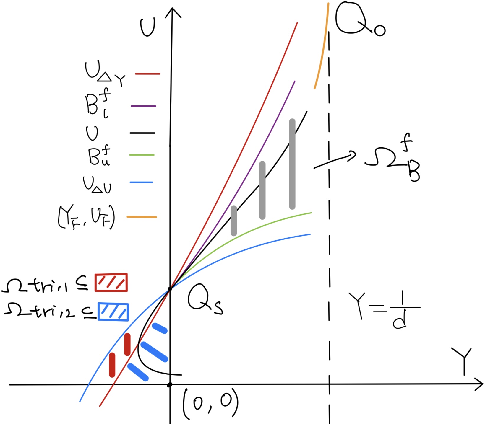
(2.24b)		$U_{\Delta_{Y}}(Y)=-\frac{(Y-1)f(Y)}{dY-1},\quad U_{\Delta_{U}}(Y)=-f(Y)-(d-1)Y(1-Y).$

See Figure 2 for an illustration of the curves $U_{\Delta_{Y}}(Y)$ (red), $U_{\Delta_{U}}(Y)$ (blue).

We have the following basic properties about $U_{\Delta_{Y}},U_{\Delta_{U}},U_{g}$ .

Lemma 2.4.

Suppose that $(d,\ell,\gamma)$ satisfies $\ell^{-1/2}<\gamma<1,3+2\ell>d,\ell<d-1$ . For $Y<0$ , we have $U_{\Delta_{Y}}^{\prime}(Y)>0,U_{\Delta_{U}}^{\prime}(Y)>0$ . For $-\gamma<Y<0$ , we have $U_{g}^{\prime}(Y)>0$ .

The above properties hold for a wider range of parameters $(\ell,d,\gamma)$ , but we restrict the range to simplify the proof. The parameters in (2.6) with $\ell^{-1/2}<\gamma<1$ satisfy the above assumptions.

Proof.

Using the definition of $f(Y)$ (2.14), we compute

	$\displaystyle U_{\Delta_{U}}^{\prime}(Y)$	$\displaystyle=-(-A+2BY)-(d-1)+2(d-1)Y=A-(d-1)+2(d-1-B)Y$
		$\displaystyle=2-(d-1-2\ell)\gamma+2(\ell-d)Y.$

Since $0<\gamma<1,\ell<d-1,3+2\ell>d$ , and $d\geq 1$ , using the formula of $A$ (2.9), we obtain

(2.25)

A\geq 2-(d-1-2\ell)\gamma>\min(2,2-(d-1-2\ell))=\min(2,3+2\ell-d)>0.

For $Y<0$ , it follows that $2-(d-1-2\ell)\gamma>0,2(\ell-d)Y>0$ , and $U_{\Delta_{U}}^{\prime}(Y)>0$ .

For $U_{g}^{\prime}$ with $Y\in(-\gamma,0)$ , we compute

	$\displaystyle U_{g}^{\prime}(Y)$	$\displaystyle=2\ell(Y+\gamma)-2(Y-1)=2(\ell-1)Y+2\ell\gamma+2$
		$\displaystyle>-2(\ell-1)\gamma+2\ell\gamma+2=2\gamma+2>0.$

For $U_{\Delta_{Y}}^{\prime}(Y)$ , we compute

U_{\Delta_{Y}}^{\prime}=\frac{C(Y)}{(dY-1)^{2}},\quad C(Y)=-((Y-1)f(Y))^{\prime}(dY-1)+d(Y-1)f(Y).

Thus, we only need to show $C(Y)>0$ . Using the formula of $f(Y)$ (2.14), we compute

	$\displaystyle(Y-1)f(Y)$	$\displaystyle=(Y-1)(-\varepsilon-AY+BY^{2})=BY^{3}-(A+B)Y^{2}+(A-\varepsilon)Y+\varepsilon,$
	$\displaystyle((Y-1)f(Y))^{\prime}$	$\displaystyle=3BY^{2}-2(A+B)Y+A-\varepsilon.$

It follows

	$\displaystyle C(Y)$	$\displaystyle=-(3BY^{2}-2(A+B)Y+A-\varepsilon)(dY-1)+d(BY^{3}-(A+B)Y^{2}+(A-\varepsilon)Y+\varepsilon)$
		$\displaystyle=-2BdY^{3}+(Ad+B(3+d))Y^{2}-2(A+B)Y+A+(d-1)\varepsilon.$

Recall $A>0$ from (2.25). Since $\gamma>\ell^{-1/2}$ and $\ell<d-1$ , we get $\varepsilon>0$ and $B=2d-1-\ell>d>0$ (2.9). Using the estimates of the sign of each term and $Y\leq 0$ , we obtain that each monomial in $C(Y)$ is non-negative for $Y\leq 0$ . Since $A+(d-1)\varepsilon>0$ , we prove $C(Y)>0$ . MM $\square$

2.4. Eigen-system near $Q_{s}$

We define

(2.26a)	$M_{Q}:=\begin{pmatrix}\partial_{U}\Delta_{U}&\partial_{Y}\Delta_{U}\\ \partial_{U}\Delta_{Y}&\partial_{Y}\Delta_{Y}\\ \end{pmatrix}\Big{\|}_{Q=Q_{s}}=\begin{pmatrix}c_{1}&c_{3}\\ c_{2}&c_{4}\\ \end{pmatrix}.$
Using the definitions in (2.14) and a direct computation, at $(Y,U)=Q_{s}=(0,\varepsilon)$ , we yield ⁴⁴4 These formulas have also been derived in [56, Sections 4.1, 4.2].

(2.26b)	$\displaystyle c_{1}$	$\displaystyle=4U+2(f(Y)+kY(1-Y))=2\varepsilon,\$	$\displaystyle c_{3}=2U(d-1-2kY-A+2BY)=2\varepsilon(d-1-A),$
(2.26b)	$\displaystyle c_{2}$	$\displaystyle=-1,\$	$\displaystyle c_{4}=dU+f(0)-(-A)=(d-1)\varepsilon+A,$

where $\varepsilon,A,B$ are defined in (2.10). The eigenvalues of $M_{Q}$ are given by


(2.27a)		$\displaystyle\lambda^{2}-(c_{1}+c_{4})\lambda+(c_{1}c_{4}-c_{2}c_{3})=0,$
(2.27a)		$\displaystyle\lambda_{\pm}=\frac{c_{1}+c_{4}\pm\sqrt{(c_{1}-c_{4})^{2}+4c_{2}c_{3}}}{2}.$
Using the above formulas of $c_{i}$ and (2.6), (2.9), we compute
(2.27b)	$\begin{gathered}c_{1}+c_{4}=(d+1)\varepsilon+A>0,\quad c_{1}c_{4}-c_{2}c_{3}=2(d-1)\varepsilon(\varepsilon+1)>0,\\ c_{3}=2\varepsilon((d-1-2\ell)\gamma-2)<0,\quad(c_{1}+c_{4})^{2}-4(c_{1}c_{4}-c_{2}c_{3})>0.\end{gathered}$

We view all the parameters as functions in $\gamma$ . From (2.27), for $\gamma>\ell^{-1/2}$ , we obtain

(2.28)

0<\lambda_{-}<\lambda_{+}.

Since $\varepsilon|_{\gamma=\ell^{-1/2}}=0$ (2.9), using the above estimates and (2.9), we obtain

(2.29)

\lim_{\gamma\to(\ell^{-1/2})^{+}}\lambda_{-}(\gamma)=0,\quad\lim_{\gamma\to(\ell^{-1/2})^{+}}\lambda_{+}(\gamma)=\lambda_{+}(\ell^{-1/2})>0.

We introduce the parameter

(2.30)

\kappa(\gamma)=\frac{\lambda_{+}}{\lambda_{-}},

related to the asymptotics of the power series of $U$ near the sonic point. Using (2.27), we obtain

(2.31)

\frac{(\kappa(\gamma)+1)^{2}}{\kappa(\gamma)}=\frac{(\lambda_{+}+\lambda_{-})^{2}}{\lambda_{+}\lambda_{-}}=\frac{(c_{1}+c_{4})^{2}}{c_{1}c_{4}-c_{2}c_{3}}=\frac{((d+1)\ell\gamma-(d-1-2\ell))^{2}}{2(d-1)\ell(\ell\gamma^{2}-1)}.

We want to study the smooth self-similar profile with $\kappa(\gamma)$ sufficiently large, which provides an important large parameter in our analysis. Since $\gamma\ell>\ell^{1/2}>1$ , the numerator is always larger than $4$ . Thus, we want to choose $\gamma>\gamma_{*}$ with $\gamma$ close to $\gamma_{*}$

(2.32)

\gamma\to(\gamma_{*})^{+},\quad\gamma_{*}=\ell^{-1/2},

which is consistent with the constraint in Lemma 2.1. Note that given $\kappa$ , we can determine $\gamma$ via (2.31). It is not difficult to see that $\kappa(\gamma)$ decreases in $\gamma$ for $\gamma\in(\ell^{1/2},\ell^{1/2}+c)$ with some absolute constant $c>0$ , $\kappa(\gamma)$ is a smooth bijection, and it admits an inverse map $\gamma=\Gamma(\kappa)$ :

(2.33)

\begin{gathered}\kappa(\gamma):I_{\gamma}\to I_{\kappa},\quad\Gamma(\kappa):I_{\kappa}\to I_{\gamma},\quad\Gamma(\kappa(\gamma))=\gamma,\\ I_{\gamma}\triangleq(\ell^{1/2},\ell^{1/2}+c),\quad I_{\kappa}\triangleq(C_{\kappa},\infty),\quad C_{\kappa}=\kappa(\ell^{1/2}+c).\end{gathered}

Thus, for each integer $n>C_{\kappa}$ , there exists strictly decreasing $\gamma_{n}>\ell^{1/2}$ such that

(2.34)

\kappa(\gamma_{n})=n>C_{\kappa}.

In the remainder of the paper, we drop the dependence of $\kappa$ on $\gamma$ for simplicity. Whenever we refer to choosing $\kappa$ sufficiently large, it is equivalent to taking $\gamma$ sufficiently close to $\ell^{-1/2}$ .

Next, we use the ODE (2.15b) to compute the slope of the solution $(Y,U(Y))$ at the sonic point $Q_{s}$ , which is given by $(1,U_{1})$ with

U_{1}=\frac{dU}{dY}\Big{|}_{Y=Y_{0}}.

Denote $\xi=Y-Y_{0}$ . Applying Taylor expansion near $Q_{s}=(Y_{0},U_{0})$ (2.26), we get

(2.35)

\Delta_{\alpha}(Y,U(Y))|_{Q_{s}}=\frac{d}{dY}\Delta_{\alpha}(Y,U(Y))\Big{|}_{Y=Y_{0}}\xi+O(\xi^{2})=(\partial_{Y}\Delta_{\alpha}+\partial_{U}\Delta_{\alpha}\cdot U_{1})\xi+O(\xi^{2}).

Using the derivation for $\nabla_{Y,U}\Delta_{\alpha}$ from (2.26) and the ODE (2.15b), we yield

(2.36)

U_{1}=\frac{c_{1}U_{1}+c_{3}}{c_{2}U_{1}+c_{4}},\quad c_{2}U_{1}^{2}+(c_{4}-c_{1})U_{1}-c_{3}=0.

It is not difficult to show that (2.36) implies that $(1,U_{1})$ is an eigenfunction of $M_{Q}$ (2.26). Moreover, using (2.26b) and (2.27b), we get $-c_{3}/c_{2}=c_{3}<0$ . Thus, the above equation has two roots $U_{1,-}<0<U_{1,+}$ . The eigenfunction associated with eigenvalue $\lambda$ is parallel to

\mathbf{u}_{\lambda}=\begin{pmatrix}c_{3}\\ \lambda-c_{1}\\ \end{pmatrix}=\begin{pmatrix}\lambda-c_{4}\\ c_{2}\\ \end{pmatrix}.

We want to construct a smooth curve that pasts through $Q_{s}$ along the positive direction $(1,U_{1,+})$ . See the black curve in Figure 2 for an illustration of the direction. Using (2.27), (2.26), (2.6), (2.9), for $\gamma$ close to $\ell^{-1/2}$ , which implies $0<\lambda_{-},\varepsilon\ll 1$ , we get that the direction $(1,U_{1,+})$ corresponds to $u_{\lambda_{-}}$ . We fix $U_{1}=U_{1,+}$ . Since $(1,U_{1})$ and $u_{\lambda_{-}}$ are parallel, we can represent $U_{1}$ and $\kappa(\gamma)$ (2.31) as follows

(2.37)

\begin{gathered}U_{1}=\frac{\lambda_{-}-c_{4}}{c_{2}},\quad\lambda_{-}=c_{2}U_{1}+c_{4},\quad\lambda_{+}=c_{1}+c_{4}-\lambda_{-}=-c_{2}U_{1}+c_{1},\\ \kappa(\gamma)=\frac{\lambda_{+}}{\lambda_{-}}=\frac{c_{1}-c_{2}U_{1}}{c_{2}U_{1}+c_{4}}.\end{gathered}

2.5. Outline of the proof

In this section, we outline the proof of Theorem 1.1.

In Section 3, we analyze the ODE (2.14) near the sonic point $Q_{s}=(Y_{0},U_{0})$ (2.16) by constructing power series solution $U(Y)$ and estimating the asymptotics of the power series coefficients $U_{n}$ using induction.

In Section 4, we use a double barrier argument, a shooting argument, to extend the local power series solution $U(Y)$ to $Y\in[-c,Y_{O}-c]$ for some small $c$ , which along with a gluing argument gives rise to a smooth ODE solution $V(Z)$ to (2.3) for $Z\in[0,Z_{0}+\varepsilon_{1}]$ with small $\varepsilon_{1}>0$ . It corresponds to a solution curve $(Z,V)$ connecting $P_{O},P_{s}$ . See the black curve in Figure 1 or the curves above $Q_{s}$ in Figure 2 for illustrations.

In Section 5, we use a barrier argument and some monotone properties to extend the local power series solution $U(Y)$ for $Y<0$ . We further study a desingularized ODE (5.34) of $(Y_{\mathrm{ds}},U_{\mathrm{ds}})$ and extend the solution curve $(Y_{\mathrm{ds}},U_{\mathrm{ds}})$ below $Q_{s}$ across $Y=0$ . See the black curve below $Q_{s}$ in Figure 2 for an illustration.

In Section 6, we glue the solutions of the $(Z,V)$ -ODE (2.3), the $(Y,U)$ -ODE (2.14), and the desingularized ODE $(Y_{\mathrm{ds}},U_{\mathrm{ds}})$ (5.34), and use some monotonicity properties of the $(Z,V)$ -ODE (2.3) to obtain a global solution to the $(Z,V)$ ODE. We then proceed to prove Theorem 1.1.

3. Power series near the sonic point

In this section, we study the behavior of the ODE (2.14) near the sonic point $Q_{s}=(Y_{0},U_{0})$ (2.16) using power series expansion

(3.1)

Y=y_{0}+\xi,\quad U\triangleq\sum_{n\geq 0}u_{n}\xi^{n}.

Although we have $Y_{0}=0$ in our case, we aim to develop a general method which does not depend on fine properties of the ODEs, e.g., specific value or degree of the polynomials.

3.1. Recursive formula

In this section, our goal is to establish Lemma 3.2 for the recursive formula of the power series coefficients $U_{i}$ of the ODE solution near the sonic point $Q_{s}=(Y_{0},U_{0})$ .

Notations

Throughout this section, we use $y_{0},u_{0},u_{1},..$ to denote variables, and $Y_{0},U_{0},U_{1},..$ to denote the value of the power series coefficients of the solution $(Y,U)$ to the ODE (2.14).

Firstly, for any two power series $A,B$ with coefficients $\{A_{n}\}_{n\geq 0},\{B_{n}\}_{n\geq 0}$ , i.e. $C(Y)=\sum_{n\geq 0}C_{n}\xi^{n},C=A,B$ , we get

(3.2)

AB=\sum_{n\geq 0}(AB)_{n}\xi^{n},\quad(AB)_{n}=\sum_{i\leq n}A_{i}B_{n-i}.

Given any power series $U$ with coefficients $\{u_{i}\}_{i\geq 0}$ and $Y=y_{0}+\xi$ (3.1), since $\Delta_{Y},\Delta_{U}$ are polynomials of $U,Y$ , using the above convolution formula, we can obtain the power series of $\Delta_{\alpha}$

(3.3)

\displaystyle\Delta_{\alpha}(Y,U)

\displaystyle=\sum_{n\geq 0}\Delta_{\alpha,n}(y_{0},u_{0},u_{1},..,u_{n})\xi^{n},\quad\alpha=U,Y.

Applying chain rule, one can obtain that $\Delta_{\alpha,n}$ only depends on $y_{0},u_{0},..,u_{n}$ . For example, we have the following formula for the first term $\Delta_{\alpha,1}$

(3.4)

\Delta_{\alpha,1}(y_{0},u_{0},u_{1})=\frac{d}{d\xi}\Delta_{\alpha}(Y,U)\Big{|}_{\xi=0}=u_{1}\cdot\partial_{U}\Delta_{\alpha}(y_{0},u_{0})+\partial_{Y}\Delta_{\alpha}(y_{0},u_{0}).

We introduce the following functions

(3.5)

c_{\alpha,j}(y_{0},u_{0},..,u_{j})\triangleq\frac{1}{j!}\Big{(}\frac{d^{j}}{d\xi^{j}}(\partial_{U}\Delta_{\alpha})(Y,U)\Big{)}\Big{|}_{\xi=0},\quad\alpha=U,\ Y.

It is easy to see that $c_{\alpha,j}$ only depends on $y_{0},u_{0},u_{1},..,u_{j}$ using the chain rule. We will use them in Lemmas 3.1, 3.2. For simplicity, we drop the dependence of $c_{\alpha,j}$ on $y_{0},u_{i}$ .

We have the following formula regarding the coefficients of $\Delta_{\alpha,n},\alpha=U,Y$ .

Lemma 3.1.

Let $c_{\alpha,i}$ be the functions defined in (3.5). For any $(i,j,n)$ with $n\geq 1,i\geq 0$ , $j>i$ , and $\alpha=U,Y$ , the coefficients $\Delta_{\alpha,\cdot}$ defined via (3.3) satisfies


(3.6a)	$\displaystyle\partial_{u_{n}}\Delta_{\alpha,n+i}(y_{0},u_{0},..,u_{n+i})$	$\displaystyle=c_{\alpha,i},$
(3.6b)	$\displaystyle\partial_{u_{j}}\partial_{u_{n}}\Delta_{\alpha,n+i}(y_{0},u_{0},..,u_{n+i})$	$\displaystyle=0.$
Specifically, $\partial_{u_{n}}\Delta_{\alpha,n+i}(y_{0},u_{0},..,u_{n+i})$ does not depend on $u_{j}$ for $j>i$ . For any $i<n$ , we have
(3.6c)	$\partial_{u_{n}}\Delta_{\alpha,i}(y_{0},u_{0},..,u_{i})=0.$

Proof.

Recall the expansion (3.1). For $i<n$ , since $\Delta_{\alpha,i}$ only depends on $y_{0},u_{0},..,u_{i}$ , we obtain (3.6c) trivially.

Since $U=\sum_{i\geq 0}u_{j}\xi^{j}$ , taking $\partial_{u_{n}}$ on both sides of (3.3) and then using (3.6b), we yield

(\partial_{U}\Delta_{\alpha})(Y,U)\cdot\xi^{n}=\sum_{j\geq n}\partial_{u_{n}}\Delta_{\alpha,j}(y_{0},u_{0},..,u_{n},..,u_{j})\xi^{j}

Matching the coefficients of $\xi^{n+i}$ on both sides and then evaluating at $\xi=0$ , we get

(3.7)

c_{\alpha,i}=\frac{1}{i!}\Big{(}\frac{d^{i}}{d\xi^{i}}(\partial_{U}\Delta_{\alpha})(Y,U\Big{)}\Big{|}_{\xi=0}=\partial_{u_{n}}\Delta_{\alpha,n+i}(y_{0},u_{0},..,u_{n+i})

and prove (3.6a). It is not difficult to see that the left hand side of (3.7) only depends on $U$ via $u_{0},u_{1},..,u_{i}$ . Therefore, if $j>i$ , we yield

\partial_{u_{j}}\partial_{u_{n}}\Delta_{\alpha,n+i}=\partial_{u_{j}}c_{\alpha,i}=0,

and prove (3.6b). MM $\square$

3.1.1. Derivation of the recursive formulas

Now, we derive the recursive formula for the power series coefficients $U_{n},n\geq 0$ of $U$ (3.1) near $Q_{s}=(Y_{0},U_{0})$ :

(3.8)

U=\sum_{i\geq 0}U_{i}\xi^{i},\quad Y=Y_{0}+\xi

with $U$ satisfying the ODE (2.3).

Firstly, recall the notations from (2.16) and (2.26). We have $Q_{s}=(U_{0},Y_{0})$ and

(3.9)

\Delta_{\alpha}(Q_{s})=0,\quad\alpha=U,Y.

Thus, the leading coefficient satisfies $\Delta_{\alpha,0}=0$ for $\alpha=U,Y$ . Using the ODE (2.3) together with the expansions (3.3) and (3.8), we obtain

\Delta_{Y}(Y,U(Y))\frac{dU}{dY}=\Delta_{U}(Y,U(Y)),\quad\frac{dU}{dY}=\sum_{i\geq 0}(i+1)\xi^{i}U_{i+1}.

Matching the coefficients of $\xi^{n}$ , we get

(3.10)

\sum_{1\leq i\leq n}\Delta_{Y,i}\cdot(n-i+1)U_{n-i+1}-\Delta_{U,n}=0,

where $\Delta_{Y,i},\Delta_{U,i}$ evaluate on $y_{0}=Y_{0},u_{j}=U_{j},j\leq i$ .

Let us define

(3.11)

\mathfrak{R}_{n}(y_{0},u_{0},..,u_{n})=\sum_{1\leq i\leq n}\Delta_{Y,i}(y_{0},u_{0},..,u_{n})\cdot(n-i+1)u_{n-i+1}-\Delta_{U,n}(y_{0},u_{0},..,u_{n}).

From (3.10), evaluating at ( $Y_{0},U_{0},..,U_{n}$ ), we have

(3.12)

\mathfrak{R}_{n}(Y_{0},U_{0},..,U_{n})=0.

Next, we derive another formula of $\mathfrak{R}_{n}$ by determining the explicit dependence on the $N$ terms $u_{n},..,u_{n-N+1}$ . Then, by evaluating $\mathfrak{R}_{n}$ on $y_{0}=Y_{0},u_{i}=U_{i},i\geq 0$ , we can obtain the recursive formula of $U_{n}$ in terms of $U_{i}$ for $i<n$ . We will choose

(3.13)

N=O(1)\ll n,\quad n-N>\frac{n}{2}+2.

When we use the recursive formula later, e.g., in Section 3.2, we choose $n\geq n_{1}$ with $(n_{1},N)$ given in (3.23).

Expansion of $\mathfrak{R}_{n}$

For $m$ with $n-N<m\leq n$ , taking $u_{m}$ derivative on (3.11) and using (3.6c), we obtain

\displaystyle\partial_{u_{m}}\mathfrak{R}_{n}

\displaystyle=\sum_{m\leq i\leq n}\partial_{u_{m}}\Delta_{Y,i}(n-i+1)u_{n-i+1}+m\Delta_{Y,n+1-m}-\partial_{u_{m}}\Delta_{U,n},

and then using (3.6a) and changing $i=m+j$ , we get

\partial_{u_{m}}\mathfrak{R}_{n}=\sum_{0\leq j\leq n-m}c_{Y,j}(n-m-j+1)u_{n+1-m-j}+m\Delta_{Y,n+1-m}-c_{U,n-m}.

These identities hold for functions $\mathfrak{R}_{n},c_{\alpha,i},\Delta_{\alpha,i}$ evaluated in any $y_{0},u_{j},j\geq 0$ .

For $m$ with $n-N<m\leq n$ and $N<(n-2)/2$ (see the bound in $N$ (3.13)), we have $n+1-m,n+1-m-j\leq N<m$ . Thus, the right-hand side of the above formula depends only on $y_{0},u_{0},u_{1},..,u_{N}$ and is independent of $u_{m}$ , and $\mathfrak{R}_{n}$ depends linearly on $u_{m}$ .

To simplify the notations, we introduce the following functions


(3.14a)	$\displaystyle e_{l}$	$\displaystyle=\sum_{0\leq j\leq l}c_{Y,j}(l+1-j)u_{l+1-j}-c_{U,l},$
where $c_{Y,j},c_{U,j}$ are defined in (3.5). Then we can rewrite $\partial_{u_{m}}\mathfrak{R}_{n}$ as follows
(3.14b)	$a_{n,m}(y_{0},u_{0},..,u_{n-m},u_{n-m+1})\triangleq\partial_{u_{m}}\mathfrak{R}_{n}=e_{n-m}+m\Delta_{Y,n-m+1}.$

The above discussion implies the following expansion of $\mathfrak{R}_{n}$ in the top $N$ terms

(3.15)

\mathfrak{R}_{n}(y_{0},u_{0},..,u_{n})=\sum_{n-N<m\leq n}a_{n,m}u_{m}+\mathfrak{R}_{n}(y_{0},u_{0},..,u_{n-N},0,..,0).

Combining (3.12) and (3.11), we have the following results.

Lemma 3.2.

Given $U_{0},Y_{0},U_{1}$ , for $2N<n-2$ , the coefficients $\{U_{i}\}_{i\geq 0}$ of the power series (3.1) solving (2.3) near $(U_{0},Y_{0})$ satisfy

(3.16)		$\displaystyle\sum_{n-N<m\leq n}a_{n,m}U_{m}$	$\displaystyle=\Delta_{U,n}(Y_{0},U_{0},..,U_{n-N},0,..,0)$
(3.16)			$\displaystyle\quad-\sum_{N+1\leq i\leq n}(n+1-i)U_{n+1-i}\Delta_{Y,i}(Y_{0},U_{0},..,U_{n-N},0..,0),$

where we abuse notation by denoting $a_{n,m}$ the value of the functions $a_{n,m}$ (3.14) evaluating on $y_{0}=Y_{0},u_{j}=U_{j}$ for $j\geq 0$ . For $m$ with $n-N<m\leq n$ , $a_{n,m}$ only depend on $Y_{0},U_{0},U_{1},..,U_{N}$ . Here, we use the convention

\Delta_{Y,i}(Y_{0},U_{0},..,U_{n-N},0..,0)=\Delta_{Y,i}(Y_{0},U_{0},..,U_{i})

if $n-N\geq i$ . In particular, for $N=1$ and $n\geq 2$ , we have

(3.17)

\displaystyle(n\lambda_{-}-\lambda_{+})U_{n}

\displaystyle=\Delta_{U,n}(Y_{0},U_{0},..,U_{n-1},0)-\sum_{2\leq i\leq n}(n+1-i)U_{n+1-i}\Delta_{Y,i}(Y_{0},U_{0},..,U_{n-1},0),

where $\lambda_{-},\lambda_{+}$ are defined in (2.27a) and the right hand side is independent of $U_{n}$ .

Recall $c_{1},c_{2}$ from (2.26). With $U_{n}$ , we can further update $\Delta_{U,n},\Delta_{Y,n}$ as follows

(3.18)		$\displaystyle\Delta_{U,n}(Y_{0},U_{0},..,U_{n-1},U_{n})$	$\displaystyle=\Delta_{U,n}(Y_{0},U_{0},..,U_{n-1},0)+c_{1}U_{n},$
(3.18)		$\displaystyle\Delta_{Y,n}(Y_{0},U_{0},..,U_{n-1},U_{n})$	$\displaystyle=\Delta_{Y,n}(Y_{0},U_{0},..,U_{n-1},0)+c_{2}U_{n}.$

Remark 3.3 (Parameters and coefficients).

Since in the rest of the paper, we only use the values of the functions $c_{\alpha,i},e_{i},a_{n,m}$ (3.5), (3.14) evaluating on $y_{0}=Y_{0},u_{j}=U_{j}$ for any $j\geq 0$ , we abuse notation by using $c_{\alpha,i},e_{i},a_{n,m}$ to denote the values.

Proof.

Evaluating (3.15) on $y_{0}=Y_{0},u_{j}=U_{j}$ for any $j\geq 0$ , and applying $\mathfrak{R}_{n}=0$ (3.10) and the definition (3.11) to $\mathfrak{R}_{n}(Y_{0},U_{0},..,U_{n-N},0,0,..,0)$ , we prove the identity (3.16). From (3.3), we know that $\Delta_{\alpha,i}$ only depends on $Y_{0},U_{0},..,U_{i}$ .

Note that the right hand side of (3.17) is the same as (3.16) with $N=1$ . Thus to prove (3.17), we only need to evaluate $a_{n,n}$ on $Y_{0},U_{j},j\geq 0$ . We first compute $c_{U,0}(Y_{0},U_{0}),c_{Y,0}(Y_{0},U_{0})$ . Using the definition (3.5) and the notations (2.26), we have

(3.19)

\begin{gathered}c_{U,0}(Y_{0},U_{0})=\partial_{U}\Delta_{U}(Y_{0},U_{0})=c_{1},\quad c_{Y,0}(Y_{0},U_{0})=\partial_{U}\Delta_{Y}(Y_{0},U_{0})=c_{2}.\end{gathered}

Using (3.14) and the formulas of $c_{U,0},c_{Y,0}$ (3.19), $\Delta_{Y,1}$ (3.4), and then $\lambda_{-},\lambda_{+}$ (2.37), we obtain

	$\displaystyle a_{n,n}$	$\displaystyle=e_{1,0}+ne_{2,0}=c_{Y,0}U_{1}-c_{U,0}+n\Delta_{Y,1}=c_{2}U_{1}-c_{1}+n(U_{1}\partial_{U}\Delta_{Y}+\partial_{Y}\Delta_{Y})$
		$\displaystyle=c_{2}U_{1}-c_{1}+n(c_{2}U_{1}+c_{4})=n\lambda_{-}-\lambda_{+},$

and prove (3.17). Using (3.6a) with $i=0$ , we obtain

\partial_{u_{n}}\Delta_{U,n}(y_{0},u_{0},..,u_{n})=c_{U,0}=c_{1},\quad\partial_{u_{n}}\Delta_{Y,n}(y_{0},u_{0},..,u_{n})=c_{Y,0}=c_{2}.

From (3.19), we obtain that $c_{1},c_{2}$ is independent of $U_{n}$ (3.19). Thus, we prove (3.18). MM $\square$

To simplify the estimate of the power series coefficients, we consider the renormalized coefficient $\hat{U}_{n}$

(3.20a)		$U_{n}=\hat{U}_{n}\mathfrak{C}_{n},\quad\mathfrak{C}_{n}=\frac{1}{n+1}\binom{2n}{n},$
where $\mathfrak{C}_{n}$ is the Catalan number and $\mathfrak{C}_{n}$ satisfies the following asymptotics and identity
(3.20b)		$\frac{\mathfrak{C}_{n+1}}{\mathfrak{C}_{n}}=\frac{4n+2}{n+2},\quad\lim_{i\to\infty}\frac{\mathfrak{C}_{i+1}}{\mathfrak{C}_{i}}=4,\quad\sum_{i=0}^{n}\mathfrak{C}_{i}\mathfrak{C}_{n-i}=\mathfrak{C}_{n+1}.$
for any $n\geq 0$ . See [62, Section 1] for the identity. Moreover, for $n\geq 4$ , we yield
(3.20c)		$3\mathfrak{C}_{n}\leq\mathfrak{C}_{n+1}<4\mathfrak{C}_{n}.$

3.2. Asymptotics of the coefficients

In this Section, we develop refine estimates of $U_{n},\hat{U}_{n}$ , which are crucial for the barrier argument Sections 4, 5. Although the relations (3.16) and (3.17) seem to be complicated, we will show that the top two terms $a_{n,n}U_{n}$ and $a_{n,n-1}U_{n-1}$ are the dominated terms and determine the asymptotics of $U_{n}$ . Other terms can be treated perturbatively. Using Lemma 3.1 and (3.14), one can show that

(3.21)

-\frac{a_{n,n-1}}{a_{n,n}}=\frac{n\kappa}{\kappa-n}\cdot\frac{\Delta_{Y,2}}{\lambda_{+}}+O(|n-\kappa|^{-1}).

We expect that the asymptotic growth rate of $U_{n}/U_{n-1}$ is given by the above rate and will justify it in (3.22e) in Lemma 3.5 and Corollary 3.11, equation (3.61).

We have the following estimate for binomial coefficients.

Lemma 3.4.

For any $n\geq 1$ and $1\leq j\leq n/2$ , we have $\binom{n}{j}\geq\frac{4^{j}}{3j^{1/2}}$ .

The proof is elementary and we refer to [6, Lemma 5.5].

We have the following estimates of the asymptotics of $\hat{U}_{n}$ . ⁵⁵5In Lemma 3.5 and its proof, we do not assume that $\kappa\in(n,n+1)$ .

Lemma 3.5.

Let $n_{0}$ be the parameter chosen in (3.23). There exists $\kappa_{0}$ large enough such that for any $\kappa>\kappa_{0}$ and $\kappa\notin\mathbb{Z}$ , the following statements hold true.

For any $0\leq j\leq n<\kappa+2$ , we get ⁶⁶6 In the upper bound of (3.22a), we use $\|\hat{U}_{n}\|$ instead of the more symmetric form $\|\hat{U}_{0}\hat{U}_{n}\|$ since $\hat{U}_{0}$ can be $0$ . In our case, we have $\hat{U}_{0},U_{0}\to 0$ (2.16) as $\gamma\to\ell^{-1/2}$ .
(3.22a)		$\|\hat{U}_{j}\hat{U}_{n-j}\|\leq\bar{C}_{1}\|\hat{U}_{n}\|,\quad\bar{C}_{1}=12.46.$

For any $n_{0}\leq n<\kappa$ , we have

(3.22b)

U_{n},\ \hat{U}_{n}>0.

For any $n_{0}\leq n<\kappa+2$ , we have

(3.22c)

|\hat{U}_{n-1}|<|\hat{U}_{n}|.

Let $\hat{\delta}=0.049$ be chosen in (2.10), and denote

(3.22d)

C_{*}=\lim_{\gamma\to(\ell^{-1/2})^{+}}\frac{\Delta_{Y,2}}{\lambda_{+}}.

For any $n$ with $n_{0}\leq n<\kappa+2$ , we get

(3.22e)

\displaystyle\Big{|}\hat{U}_{n}-\frac{C_{*}}{4}\cdot\frac{n\kappa}{\kappa-n}\hat{U}_{n-1}\Big{|}

\displaystyle\leq\hat{\delta}\Big{|}\frac{C_{*}}{4}\cdot\frac{n\kappa}{\kappa-n}\hat{U}_{n-1}\Big{|},

In (3.22a), (3.22c), (3.22e), we consider the range of $n$ : $n<\kappa+2$ larger than $n<\kappa$ for later estimates in Section 4. From (3.22e), for $n>\kappa$ , $U_{n}$ changes sign, and (3.22b) does not hold.

Ideas and strategy

We expect that the asymptotics of $\hat{U}_{n}$ is given by (3.22e), which quantifies the growth rate (3.21) for $U_{n}/U_{n-1}$ . Since $|U_{i}|$ grows very fast in $i$ , we can treat the remaining terms $U_{i},i\leq n-2$ in (3.17), (3.16) perturbatively.

Recall $d_{Y},d_{U}$ from (2.15a). To prove the induction, we introduce a few parameters

(3.23)

l_{0}=\max(d_{Y},d_{U})=2,\quad n_{0}=20,\quad j_{0}=25,\quad N=30,\quad n_{1}=450.

We require $n\geq n_{0}$ in (3.22b)-(3.22e) with $n_{0}$ not too small, since these estimates may not hold true for small $n$ . We list a few conditions satisfying by the parameters (3.23) in the following lemma. We verify them with computer assistance and will use them to prove Lemma 3.5. See more discussions on the computer assistance in Appendix B.

Lemma 3.6 (Computer-assisted).

Let $l_{0},j_{0},n_{0},n_{1}$ be the parameters in (3.24), $C_{*}$ in (3.22d), and $\bar{C}_{1}$ in (3.22a). For $\gamma=\ell^{-1/2}$ (thus $\kappa=\infty$ (2.31)), the following statements hold true.

(a) Inequality (3.22a) holds true for any $0\leq n\leq n_{1}$ , (3.22b),(3.22c),(3.22e) hold true for any $n_{0}\leq n\leq n_{1}$ , and $\bar{C}_{1}>\max(1,|\hat{U}_{0}|)$ .

(b) For any $j,l$ with $1\leq j\leq j_{0},0\leq l\leq l_{0}$ , we have

(3.24)

(\frac{C_{*}}{4}(1-\hat{\delta}))^{j-1}(n_{1}+1-N-j_{0})^{j-1}\geq 2^{j-1}\frac{|\hat{U}_{j+l-1}|}{\max(|\hat{U}_{l}|,1)}.

(3.25)

M_{1}\triangleq\sup_{l\leq l_{0}}\frac{|\hat{U}_{n_{0}}|}{n_{0}!\max(|\hat{U}_{l}|,1)}(\frac{C_{*}}{4})^{l-n_{0}},\quad\Big{(}\frac{1}{j_{0}+l_{0}}\Big{)}^{l_{0}}\cdot\frac{1}{M_{1}}\cdot\frac{(\frac{9}{5})^{j_{0}}}{3j_{0}^{1/2}}>1.

Let us motivate the choice of the parameters in (3.23). First, we fix $l_{0}$ as in (3.23). Next, we choose $n_{0}$ large enough so that conditions (3.22e), (3.22c), and (3.22b) begin to hold. We then choose $j_{0}$ large enough to verify (3.25). With $(j_{0},l_{0})$ fixed, (3.24) holds for any $n_{1},N$ with $n_{1}-N\geq n^{*}(j_{0},l_{0})$ . We choose $N$ large and then take $n_{1}=n_{1}(N)\geq n^{*}(j_{0},l_{0})+N$ to be sufficiently large. See the discussion below (3.47).

Using (3.17) and (2.29), we can obtain that $U_{n}$ is continuous in $\gamma$ as $\gamma\to\ell^{-1/2}$ for any $n\leq n_{1}$ . With Lemma 3.6 and continuity of $U_{n}$ in $\gamma$ , Lemma 3.5 holds for all $n\leq n_{1}$ and $\kappa$ large enough (equivalent to $\gamma-\ell^{-1/2}$ small). Below, we assume that the inductive hypothesis is true for the case of $\leq n-1$ and we will prove the case of $n$ with $n>n_{1}>n_{0}+2N$ . In Section 3.3, we derive the consequence of the inductive hypothesis. In Section 3.4, we estimate the coefficients of the power series of $\Delta_{U},\Delta_{Y}$ . In Section 3.5.4, we estimate $\hat{U}_{n}$ and prove the induction.

Remark 3.7.

The proof presented below does not take advantage of the specific forms of $\Delta_{Y},\Delta_{U}$ , which are polynomials in $U$ with low degree $(\leq 2)$ . We can prove it by checking the desired properties of $U_{i},i\leq n_{1}$ with $n_{1}$ large enough with computer assistance and then use induction to prove the properties of $U_{i}$ with large enough $i$ .

Constants in the estimates

Recall the constants $e_{l}$ from (3.14). In later proof, we will use the following constants, which have size of $O(1)$ compared to $\kappa$ and $n$


(3.26a)	$\displaystyle b_{2,l}$	$\displaystyle=\bar{C}_{1}^{l}\max(\|\hat{U}_{1}\|,1),\ l\geq 0,\quad b_{2,-1}=1,\quad b_{3}=\max_{i\leq N,0\leq l\leq l_{0}}\Big{\|}\frac{\hat{U}_{i}}{\hat{U}_{i+l}}\Big{\|},$
(3.26b)	$\displaystyle q_{n}$	$\displaystyle=\frac{1}{4}(n-N)(1-\hat{\delta})C_{*}.$

We use $b_{2,l}$ to denote the constants in the estimates of $U_{\mathrm{TR},j}^{l}$ in (3.38) for $l\geq 0$ . The special value $b_{2,-1}$ is used to denote the constant in the exceptional case. The parameter $b_{3}$ is used to denote the constant in (3.44). We use $q_{n}$ to denote the decay rate in the estimates of $\hat{U}_{j},U_{\mathrm{TR,j}}^{l}$ in (3.40).

3.3. Consequence of the inductive hypothesis

Suppose that the inductive hypothesis holds true for the case of $\leq n-1$ and $\kappa+2>n\geq n_{1}$ . We show that for $(l,j,m)$ with

(3.27)

0\leq l\leq l_{0}<j_{0},\quad 1\leq j,\quad j+l\leq m,\quad n_{1}-N\leq m\leq n<\kappa+2,

where $l_{0},j_{0},n_{1}$ are chosen in (3.23), we have the inequality ⁷⁷7 We use $\max(|\hat{U}_{l}|,1)|\hat{U}_{m-1}|$ instead of $|\hat{U}_{l}\hat{U}_{m-1}|$ in the upper bound since $\hat{U}_{l}$ would be $0$ .


(3.28a)	$\displaystyle\|\hat{U}_{j+l-1}\hat{U}_{m-j}\|$	$\displaystyle\leq\max(\|\hat{U}_{l}\|,1)\|\hat{U}_{m-1}\|2^{-\min(j-1,m-j-l)}.$
The estimate is trivial if $m-j=m-1$ or $j+l-1=m-1$ . Due to (3.27), it remains to consider $m-j,j+l-1\leq m-2<\kappa$ . Since (3.28a) is symmetric in $j+l-1$ and $m-j$ , we may without loss of generality assume
(3.28b)	$j+l-1\leq m-j\ \leq m-2.$

Since $0\leq l\leq l_{0}$ , $n_{0}\leq m<\kappa+2$ , from the choices of $l_{0},n_{0}$ in (3.23), we get

(3.28c)

j\leq(m+1)/2<\kappa-2.

To prove (3.28), we bound $|\frac{\hat{U}_{m-1}}{\hat{U}_{m-j}}|$ from below and $\frac{|\hat{U}_{j+l-1}|}{\max(|\hat{U}_{l}|,1)}$ from above. Since $m\geq n_{1}-N\geq 2n_{0}+2$ due to (3.23) and $1\leq j\leq(m+1)/2$ , using (3.22e) repeatedly, we get

(3.29)

\displaystyle\Big{|}\frac{\hat{U}_{m-1}}{\hat{U}_{m-j}}\Big{|}\geq(\frac{C_{*}(1-\hat{\delta})}{4})^{j-1}\prod_{m+1-j\leq i\leq m-1}\Big{|}\frac{i\kappa}{\kappa-i}\Big{|}\geq(\frac{C_{*}(1-\hat{\delta})}{4})^{j-1}\frac{(m-1)!}{(m-j)!}\prod_{m+1-j\leq i\leq m-2}\Big{|}\frac{\kappa}{\kappa-i}\Big{|},

where in the last inequality, we have used $|\frac{\kappa}{\kappa-(m-1)}|>1$ since

|\kappa-(m-1)|<\max(\kappa-(m-1),m-1-\kappa)<\kappa

for $n_{1}-N\leq m<\kappa+2$ . Since we consider $m\leq n<\kappa+2$ , $\kappa-(m-1)$ can be negative.

Recall $j_{0},l_{0},n_{0}$ from (3.23) and $M_{1}$ from (3.25):

(3.30)

M_{1}=\sup_{l\leq l_{0}}\frac{|\hat{U}_{n_{0}}|}{n_{0}!\max(|\hat{U}_{l}|,1)}(\frac{C_{*}}{4})^{l-n_{0}}.

The parameter $M_{1}$ can be seen as the accumulated error between the actual ratio $|\hat{U}_{n_{0}}|/|\hat{U}_{l}|$ and the desired asymptotics in (3.22e) with $\kappa$ much larger than $n_{0},l$ . Next, we estimate $\frac{|\hat{U}_{j+l-1}|}{\max(|\hat{U}_{l}|,1)}$ from above and consider $j\geq j_{0}+1$ and $j\leq j_{0}$ .

Case 1: $j\geq j_{0}+1$

Since $j_{0}\geq n_{0}\geq l_{0}\geq l$ due to (3.23) and (3.27), we get

\displaystyle\frac{|\hat{U}_{j+l-1}|}{\max(|\hat{U}_{l}|,1)}=\Big{|}\frac{\hat{U}_{j+l-1}}{\hat{U}_{n_{0}}}\cdot\frac{\hat{U}_{n_{0}}}{\max(|\hat{U}_{l}|,1)}\Big{|}\leq(1+\hat{\delta})^{j+l-1-n_{0}}(\frac{C_{*}}{4})^{j-1}\prod_{n_{0}+1\leq i\leq j+l-1}\frac{i\kappa}{\kappa-i}\cdot n_{0}!M_{1}.

Each product is non-negative since $j+l-1\leq m-2<\kappa$ (3.28b), (3.27). Moreover, since $l+2\leq l_{0}+2<n_{0}+1$ (3.23) and $\frac{\kappa}{\kappa-i}>1$ for $i<\kappa$ , we obtain

\frac{|\hat{U}_{j+l-1}|}{\max(|\hat{U}_{l}|,1)}\leq(\frac{1}{4}(1+\hat{\delta})C_{*})^{j-1}(j+l-1)!\prod_{l+2\leq i\leq j+l-1}\frac{\kappa}{\kappa-i}\cdot M_{1}.

Since $\frac{\kappa}{\kappa-i}$ for $i\leq m-2<\kappa$ (3.27), (3.28b) is increasing in $i$ and $j+l-1\leq m-2$ , we yield

(3.31)

\frac{|\hat{U}_{j+l-1}|}{\max(|\hat{U}_{l}|,1)}\leq(\frac{1}{4}(1+\hat{\delta})C_{*})^{j-1}(j+l-1)!\prod_{m+1-j\leq i\leq m-2}\frac{\kappa}{\kappa-i}\cdot M_{1}.

Combining the estimates (3.29), (3.31), setting

I=\frac{\max(|\hat{U}_{l}|,1)\cdot|\hat{U}_{m-1}|}{|\hat{U}_{j+l-1}\hat{U}_{m-j}|},

we have

I\geq\frac{1}{M_{1}}\frac{(m-1)!}{(m-j)!(j+l-1)!}\frac{(1-\hat{\delta})^{j-1}}{(1+\hat{\delta})^{j-1}}=\frac{1}{M_{1}}\binom{m-1}{j-1}\frac{(1-\hat{\delta})^{j-1}}{(1+\hat{\delta})^{j-1}}\cdot\frac{1}{(j+l-1)(j+l-2)\cdots j}.

We want to show that $I\geq 2^{j-1}$ . Since $l\leq l_{0}$ (3.27) and $j-1\geq j_{0}$ in this case, using $j+l_{0}-1\leq(j_{0}+l_{0})\frac{j-1}{j_{0}}$ , we obtain

(j+l-1)(j+l-2)\cdots j\leq(j+l_{0}-1)^{l_{0}}\leq\Big{(}\frac{j_{0}+l_{0}}{j_{0}}\Big{)}^{l_{0}}(j-1)^{l_{0}}\,.

In addition, since $j-1\leq\frac{m-1}{2}$ (3.28b), Lemma 3.4 implies

\binom{m-1}{j-1}\geq\frac{4^{j-1}}{3{(j-1)}^{1/2}}.

Combining the above estimates, we derive

	$\displaystyle I$	$\displaystyle\geq\Big{(}\frac{j_{0}}{j_{0}+l_{0}}\Big{)}^{l_{0}}\frac{1}{(j-1)^{l_{0}}}\cdot\frac{1}{M_{1}}\cdot\frac{4^{j-1}}{3(j-1)^{1/2}}\cdot\frac{(1-\hat{\delta})^{j-1}}{(1+\hat{\delta})^{j-1}}$
		$\displaystyle=\Big{(}\frac{j_{0}}{j_{0}+l_{0}}\Big{)}^{l_{0}}\cdot\frac{1}{M_{1}}\cdot\frac{4^{j-1}}{3(j-1)^{1/2+l_{0}}}\cdot\frac{(1-\hat{\delta})^{j-1}}{(1+\hat{\delta})^{j-1}}.$

Due to the choices of $j_{0},l_{0}$ in (3.23), for any $j>j_{0}$ , we have $j-1\geq j_{0}>2l_{0}+1$ . Since $\frac{2(1-\hat{\delta})}{1+\hat{\delta}}>\frac{9}{5}$ and $(\log\frac{9}{5})\cdot(j-1)\geq 2(\log\frac{9}{5})(l_{0}+\frac{1}{2})>l_{0}+\frac{1}{2}$ , we obtain that $\frac{(\frac{9}{5})^{j-1}}{(j-1)^{1/2+l_{0}}}$ is increasing in $j$ . Thus, we obtain

(3.32)

I\geq 2^{j-1}\Big{(}\frac{j_{0}}{j_{0}+l_{0}}\Big{)}^{l_{0}}\cdot\frac{1}{M_{1}}\cdot\frac{(\frac{9}{5})^{j_{0}}}{3j_{0}^{1/2+l_{0}}}=2^{j-1}\Big{(}\frac{1}{j_{0}+l_{0}}\Big{)}^{l_{0}}\cdot\frac{1}{M_{1}}\cdot\frac{(\frac{9}{5})^{j_{0}}}{3j_{0}^{1/2}}.

Recall $(l_{0},j_{0})$ from (3.23). We use the condition (3.25) in Lemma 3.6 to obtain $I\geq 2^{j-1}$ .

Case 2: $j\leq j_{0}$

Applying $|\frac{\kappa}{\kappa-i}|>1$ for $i<\kappa+2$ , $j\leq j_{0}$ , and $n_{1}-N\leq m$ to (3.29), we get

|\frac{\hat{U}_{m-1}}{\hat{U}_{m-j}}|\geq(\frac{1}{4}C_{*}(1-\hat{\delta}))^{j-1}(m+1-j_{0})^{j-1}\geq(\frac{1}{4}C_{*}(1-\hat{\delta}))^{j-1}(n_{1}+1-N-j_{0})^{j-1}.

Using the above estimate and (3.24), we obtain (3.28)

\Big{|}\frac{\hat{U}_{m-1}}{\hat{U}_{m-j}}\Big{|}\geq 2^{j-1}\frac{|\hat{U}_{j+l-1}|}{\max(|\hat{U}_{l}|,1)}.

3.4. Estimate of $\Delta_{\alpha,i}$

We will use (3.16) to estimate the coefficients $\hat{U}_{n}$ . Below, we estimate $\Delta_{\alpha,i}(Y_{0},U_{0},..,U_{n-N},0..,0)$ . We introduce the truncated power series of $U$ up to $\xi^{n-N}$

(3.33)

U_{\mathrm{TR}}:=\sum_{j\leq n-N}U_{j}\xi^{j}.

Since we choose $N$ in (3.23) and fix $n$ in the following estimates, to simplify the notation, we drop the dependence of $U_{\mathrm{TR}}$ on $n,N$ . Note that the above power series involves $U_{i}$ rather than $\hat{U}_{i}$ . We recall the relation between $U_{i},\hat{U}_{i}$ from (3.20).

Denote by $U_{\mathrm{TR},j}^{l}$ the coefficient of $\xi^{j}$ in the power series expansion of $(U_{\mathrm{TR}})^{l}$ . Next, we estimate $U_{\mathrm{TR},j}^{l}$ for $l=0,1,...,\max(d_{Y},d_{U})$ (2.15a) and $j\leq n$ .

For $l\geq 2$ and $j\leq n$ , we get

(3.34)

U_{\mathrm{TR},j}^{l}=\sum_{i_{1}+i_{2}+\cdots+i_{l}=j,\ i_{s}\leq n-N}U_{i_{1}}U_{i_{2}}\cdots U_{i_{l}}=\sum_{i_{1}+i_{2}+\cdots+i_{l}=j,\ i_{s}\leq n-N}\hat{U}_{i_{1}}\hat{U}_{i_{2}}\cdots\hat{U}_{i_{l}}\mathfrak{C}_{i_{1}}\mathfrak{C}_{i_{2}}\cdots\mathfrak{C}_{i_{l}}.

We use the inductive hypothesis to obtain two estimates of $\hat{U}_{i_{1}}\hat{U}_{i_{2}}\cdots\hat{U}_{i_{l}}$ with $l\geq 2$ . The first estimate applies to $n-N<j\leq n$ and the second applies to $j\leq n-1$ .

First estimate with $n-N<j\leq n$ .

Without loss of generality, we assume $i_{1}\leq i_{2}\leq\cdots\leq i_{l}$ . Since $i_{l}\geq 1,i_{1}+i_{2}+\cdots+i_{l}=j$ and $j\leq n$ , we get $i_{1},\cdots,i_{l-1}\leq n-1$ . Using (3.22a) repeatedly, we get

(3.35)

\displaystyle|\hat{U}_{i_{1}}\hat{U}_{i_{2}}\cdots\hat{U}_{i_{l-1}}|\leq\bar{C}_{1}^{l-2}|\hat{U}_{i_{1}+i_{2}+\cdots+i_{l-1}}|.

Due to $i_{l}=\max_{k<l}i_{k}$ , the constraint on $i_{k}$ (3.34), and $n\geq n_{1}>N(1+l_{0})$ by the choices of $n_{1},l_{0},N$ (3.23), we obtain that $i_{k}$ satisfies

(3.36)

n-N\geq i_{l}\geq\frac{n-N}{l}\geq\frac{n-N}{l_{0}}>N,\quad i_{1}+..+i_{l-1}=j-i_{l}\leq n-N.

It is easy to verify that the conditions (3.27) hold for $(l,j,m)\to(1,i_{1}+i_{2}+\cdots+i_{l-1},j)$ . Thus, using (3.28) with $(l,j,m)\to(1,i_{1}+i_{2}+\cdots+i_{l-1},j)$ and (3.35), we yield

	$\displaystyle\|\hat{U}_{i_{1}}\hat{U}_{i_{2}}\cdots\hat{U}_{i_{l-1}}\hat{U}_{i_{l}}\|$	$\displaystyle\leq\bar{C}_{1}^{l-2}\|\hat{U}_{i_{1}+i_{2}+\cdots+i_{l-1}}\hat{U}_{i_{l}}\|$
		$\displaystyle\leq\bar{C}_{1}^{l-2}\max(\|\hat{U}_{1}\|,1)\|\hat{U}_{j-1}\|\max(2^{-(i_{l}-1)},2^{-(j-i_{l}-1)}).$

Since $j$ satisfies $j-1\geq n-N\geq n_{1}-N>n_{0}$ due to (3.23), we use (3.22c) to obtain $|\hat{U}_{j-1}|\leq|\hat{U}_{n-1}|$ . From (3.36), we have

i_{l}-1\geq N-1\geq N-1+j-n,\quad j-i_{l}-1\geq j-(n-N)-1=N-1+j-n,

Thus the above estimate imply

(3.37a)		$\|\hat{U}_{i_{1}}\hat{U}_{i_{2}}\cdots\hat{U}_{i_{l-1}}\hat{U}_{i_{l}}\|\leq\bar{C}_{1}^{l-2}2^{-(j+N-n-1)}\max(\|\hat{U}_{1}\|,1)\|\hat{U}_{n-1}\|=2^{-(j+N-n-1)}b_{2,l-2}\|\hat{U}_{n-1}\|,$
where $b_{2,l}$ is defined in (3.26).

Second estimate with $j\leq n-1$ .

Using (3.22a) and $i_{1}+i_{2}+\cdots+i_{l}=j\leq n-1$ , we get another estimate

(3.37b)

|\hat{U}_{i_{1}}\hat{U}_{i_{2}}\cdots\hat{U}_{i_{l-1}}\hat{U}_{i_{l}}|\leq\bar{C}_{1}^{l-1}|\hat{U}_{j}|.

Using the identity for the Catalan number (3.20b) repeatedly, we get

(3.37c)

\sum_{i_{1}+i_{2}+\cdots+i_{l}=j,i_{s}\leq n-N}\mathfrak{C}_{i_{1}}\mathfrak{C}_{i_{2}}\cdots\mathfrak{C}_{i_{l}}\leq\sum_{a+i_{3}+\cdots+i_{l}=j+1,i_{s}\leq n-N}\mathfrak{C}_{a}\mathfrak{C}_{i_{3}}\cdots\mathfrak{C}_{i_{l}}\leq...\leq\mathfrak{C}_{j+l-1}.

Plugging the above estimates (3.37) in (3.34), for $l\geq 2$ , we obtain


(3.38a)	$\displaystyle\|U_{\mathrm{TR},j}^{l}\|$	$\displaystyle\leq\bar{C}_{1}^{l-1}\|\hat{U}_{j}\|\mathfrak{C}_{j+l-1},$	$\displaystyle j\leq n-1,$
(3.38b)	$\displaystyle\|U_{\mathrm{TR},j}^{l}\|$	$\displaystyle\leq b_{2,l-2}2^{-(j+N-n-1)}\|\hat{U}_{n-1}\|\mathfrak{C}_{j+l-1},$	$\displaystyle n-N<j\leq n.$

For $l=1$ , we just use the definition (3.33) and (3.20) to obtain the $j-$ th coefficient of $U_{\mathrm{TR}}$ : $U_{\mathrm{TR},j}^{l}=U_{\mathrm{TR},j}=U_{j}\mathbf{1}_{j\leq n-N}=\mathfrak{C}_{j}\hat{U}_{j}\mathbf{1}_{j\leq n-N}$ . Since we define $b_{2,-1}=1$ (3.26a), the above estimates hold trivially for $l=1$ .

Remark 3.8.

The estimate (3.38b) applies to $j=n$ . We will only use this estimate in Section 3.5.2 to bound $J_{2},J_{3}$ (3.41), which involves $U_{\mathrm{TR},n}^{l}$ .

For $n-N<j\leq n-1$ and any $n>n_{1}$ , using (3.22e), we get

(3.39)

|\hat{U}_{j}|<(\frac{1}{4}(n-N)(1-\hat{\delta})C_{*})^{-(n-1-j)}|\hat{U}_{n-1}|=q_{n}^{-(n-1-j)}|\hat{U}_{n-1}|<q_{n_{1}}^{-(n-1-j)}|\hat{U}_{n-1}|,

where we have used $q_{n}>q_{n_{1}}$ for $n>n_{1}$ in the last inequality since $q_{n}$ defined in (3.26) is increasing in $n$ . Moreover, $q_{n}$ is of order $n$ . Combining (3.39) and (3.38a), we obtain another estimate of $|U_{\mathrm{TR},j}^{l}|$ , which along with (3.38b) imply

(3.40)

|U_{\mathrm{TR},j}^{l}|<\mathfrak{C}_{j+l-1}|\hat{U}_{n-1}|\min\Big{(}\bar{C}_{1}^{l-1}q_{n_{1}}^{-(n-1-j)},\ b_{2,l-2}2^{-(j+N-n-1)}\Big{)},

for $n-N<j\leq n-1$ .

3.5. Proof of the induction

We decompose the right side (RS) of (3.16) into three parts as follows: the first term, the summation over $i$ with $N+1\leq i\leq n-1$ and with $i=n$

(3.41)	$\displaystyle\mathrm{RS}$	$\displaystyle=J_{3}-J_{1}-J_{2},$
	$\displaystyle J_{1}$	$\displaystyle=\sum_{N+1\leq i\leq n-1}(n+1-i)U_{n+1-i}\Delta_{Y,i}(Y_{0},U_{0},...,U_{n-N},0,0),$
	$\displaystyle\quad J_{2}$	$\displaystyle=U_{1}\Delta_{Y,n}(Y_{0},U_{0},...,U_{n-N},0,0),$
	$\displaystyle J_{3}$	$\displaystyle=\Delta_{U,n}(Y_{0},U_{0},...,U_{n-N},0,0).$

We estimate $J_{i}$ in Sections 3.5.1, 3.5.2, and the lower order terms on the left side of (3.16) in Section 3.5.3. Our goal is to show that they are small compared to $n|\hat{U}_{n-1}\mathfrak{C}_{n-1}|$ , e.g.,

|J_{i}|\ll n|\hat{U}_{n-1}\mathfrak{C}_{n-1}|.

We combine these estimates to prove the induction in Section 3.5.4.

3.5.1. Estimate of $J_{1}$

Recall $\Delta_{Y}(Y,U_{\mathrm{TR}})=\sum_{l\leq d_{Y}}G_{l}(Y)(U_{\mathrm{TR}})^{l}$ from (2.15b). Expanding the coefficients of $\Delta_{Y,i}$ using (3.2), we get

(3.42)

\displaystyle|J_{1}|

\displaystyle\leq\Big{|}\sum_{N+1\leq i\leq n-1}\sum_{0\leq l\leq d_{Y}}\sum_{j\leq\min(i,\deg G_{l})}(n+1-i)U_{n+1-i}(G_{l})_{j}U_{\mathrm{TR},i-j}^{l}\Big{|},

where $a_{i}$ denotes the $i$ -th order coefficient of in the power series of $a$ . For $l=0$ , since $(U_{\mathrm{TR}})^{0}=1$ and $N+1>d_{G}\geq\deg G_{l}$ from the definitions (3.23) of $N$ and (2.15c) for $d_{G}$ , we get

(G_{l})_{j}U_{\mathrm{TR},i-j}^{l}\mathbf{1}_{j\leq\deg G_{l},N+1\leq i}=(G_{l})_{j}\mathbf{1}_{i=j}\mathbf{1}_{j\leq\deg G_{l},N+1\leq i}=(G_{l})_{i}\mathbf{1}_{N+1\leq i\leq\deg G_{l}}=0.

Therefore, we may restrict the summation to $l\geq 1$ in (3.42). Next, we estimate

(3.43)

I_{i,j,l}\triangleq|U_{n+1-i}U_{\mathrm{TR},i-j}^{l}|=\mathfrak{C}_{n+1-i}|\hat{U}_{n+1-i}U_{\mathrm{TR},i-j}^{l}|

and consider $(i,j)$ with $n-N<i-j\leq n-1$ and $i-j\leq n-N,i\geq N+1$ separately. We have $i\geq N+1$ due to the constraint in (3.42). Since we fix $n$ below, we drop the dependence on $n$ .

Case 1: $n-N<i-j\leq n-1$

In this case, using (3.40), we get

\displaystyle I_{i,j,l}

\displaystyle\leq\mathfrak{C}_{n+1-i}\mathfrak{C}_{i-j+l-1}|\hat{U}_{n+1-i}\hat{U}_{n-1}|\min(\bar{C}_{1}^{l-1}q_{n_{1}}^{-(n-1-(i-j))},b_{2,l-2}2^{-(i-j+N-n-1)}),

In this case, since $n+1-i\leq N$ and $n+1-(i-j)\leq N+l_{0}$ ( $j\leq d_{G}\leq l_{0}$ (3.23)), we can bound $|\hat{U}_{n+1-i}/\hat{U}_{n+1-i+j}|$ by some constant $b_{3}$ (3.26) independent of $n$ and obtain

\displaystyle I_{i,j,l}

\displaystyle\leq b_{3}|\hat{U}_{n+1-(i-j)}|\mathfrak{C}_{n+1-i}\mathfrak{C}_{i-j+l-1}|\hat{U}_{n-1}|\min(\bar{C}_{1}^{l-1}q_{n_{1}}^{-(n-1-(i-j))},b_{2,l-2}2^{-(i-j+N-n-1)}).

Denote

m=n-1-(i-j).

From the bound of $i-j$ , we get $0\leq m\leq N-2$ and can further estimate $I_{i,j,l}$ as follows

(3.44)		$\displaystyle I_{i,j,l}$	$\displaystyle=b_{3}\|\hat{U}_{m+2}\|\mathfrak{C}_{n+1-i}\mathfrak{C}_{i-j+l-1}\|\hat{U}_{n-1}\|\min(\bar{C}_{1}^{l-1}q_{n_{1}}^{-m},b_{2,l-2}q^{-(N-2-m)})$
(3.44)			$\displaystyle\leq b_{3}\mathfrak{C}_{n+1-i}\mathfrak{C}_{i-j+l-1}\|\hat{U}_{n-1}\|\max_{0\leq m\leq N-2}\Big{(}\|\hat{U}_{m+2}\|\min(\bar{C}_{1}^{l-1}q_{n_{1}}^{-m},b_{2,l-2}2^{-(N-2-m)})\Big{)}.$

The bound in the maximum is very small by choosing $N$ relatively large and then $n_{1}$ large.

Case 2: $i-j\leq n-N,i\geq N+1$ .

In this case, since $i\geq N+1$ , which implies $i-j>N-l_{0}>0$ (3.23), applying (3.38) to $U_{\mathrm{TR},i-j}^{l}$ , we estimate $I_{i,j,l}$ (3.43) as

(3.45a)

I_{i,j,l}=\mathfrak{C}_{n+1-i}|\hat{U}_{n+1-i}U_{\mathrm{TR},i-j}^{l}|\leq\mathfrak{C}_{n+1-i}\mathfrak{C}_{i-j+l-1}\bar{C}_{1}^{l-1}|\hat{U}_{n+1-i}\hat{U}_{i-j}|.

If $j\leq 1$ , using (3.28) with $l=2-j$ , $i\geq N+1$ , and $i-j\leq n-N$ again, we obtain

(3.45b)		$\displaystyle\|\hat{U}_{n+1-i}\hat{U}_{i-j}\|$	$\displaystyle\leq\|\hat{U}_{n-1}\|\max(\|\hat{U}_{2-j}\|,1)2^{-\min(n-1-(n+1-i),n-1-(i-j))}$
(3.45b)			$\displaystyle\leq\|\hat{U}_{n-1}\|\max(\|\hat{U}_{2-j}\|,1)2^{-(N-1)}.$

If $2\leq j\leq\deg G_{l}$ , using (3.28) with $l=0$ , similarly, we get

\displaystyle|\hat{U}_{n+1-i}\hat{U}_{i-j}|

\displaystyle\leq|\hat{U}_{n+1-j}|\max(|\hat{U}_{0}|,1)2^{-\min(i-j,n+1-i)}.

Since $\deg G_{l}\leq d_{G}$ (see (2.15c)), $i$ satisfies $i-j\leq n-N$ and $i\geq N+1$ , we obtain

i-j\geq N+1-d_{G},\quad n+1-i\geq N-j+1\geq N+1-d_{G},\quad\min(i-j,n+1-i)\geq N+1-d_{G}.

Since $n$ satisfies $n-1\geq n+1-j\geq n_{1}+1-l_{0}>n_{0}$ , we use (3.22c) to obtain $|\hat{U}_{n+1-j}|\leq|\hat{U}_{n-1}|$ . Using the above three estimates, we simplify the bound as

(3.45c)

|\hat{U}_{n+1-i}\hat{U}_{i-j}|\leq|\hat{U}_{n-1}|\max(|\hat{U}_{0}|,1)2^{-(N+1-d_{G})}.

Combining the estimates in (3.45), we establish

(3.46)

I_{i,j,l}\leq 2^{-N}\max\Big{(}\max(|\hat{U}_{0}|,1)2^{d_{G}-1},2\max_{m\leq 2}(\max(|\hat{U}_{m}|,1))\Big{)}\mathfrak{C}_{n+1-i}\mathfrak{C}_{i-j+l-1}|\hat{U}_{n-1}|.

Summary

Summing two estimates of $I_{ijl}$ (3.44), (3.46) for two cases, we establish

(3.47)

|I_{i,j,l}|\leq\nu_{l}\mathfrak{C}_{n+1-i}\mathfrak{C}_{i-j+l-1}|\hat{U}_{n-1}|,\\

for any $l\geq 1$ , where $\nu_{l}$ is defined as

(3.48)		$\displaystyle\nu_{l}$	$\displaystyle\triangleq b_{3}\max_{0\leq m\leq N-2}\Big{(}\|\hat{U}_{m+2}\|\min(\bar{C}_{1}^{l-1}q_{n_{1}}^{-m},b_{2,l-2}2^{-(N-2-m)})\Big{)}$
(3.48)			$\displaystyle\quad+2^{-N}\max\Big{(}\max(\|\hat{U}_{0}\|,1)2^{d_{G}-1},2\max_{m\leq 2}(\max(\|\hat{U}_{m}\|,1))\Big{)},$

and $b_{2,l-2},q_{n_{1}}$ are defined in (3.26). The first term in $\nu_{l}$ corresponds to the bound (3.44) for Case 1, and the second term for the bound (3.46) in Case 2.

Since $q_{n_{1}}$ defined in (3.26b) is of order $n_{1}$ , by first choosing $N$ large so that the second part in $\nu_{l}$ is small and then $n_{1}$ large ⁸⁸8 Choosing $n_{1}$ large means that we verify the estimates in Lemma 3.5 with computer assistance up to the case $n\leq n_{1}$ with large $n_{1}$ . so that the first part is small, we can make $\nu_{l}$ very small. Therefore, combining the above estimates, we can estimate $J_{1}$ as follows

|J_{1}|\leq n\sum_{N+1\leq i\leq n-1}\sum_{1\leq l\leq d_{Y},j\leq\deg G_{l}}|(G_{l})_{j}|\nu_{l}\mathfrak{C}_{n+1-i}\mathfrak{C}_{i-j+l-1}|\hat{U}_{n-1}|.

Summing over $i$ using (3.20b) for $\mathfrak{C}_{i}$ , we yield

(3.49a)		$\|J_{1}\|\leq\sum_{1\leq l\leq d_{Y},j\leq\deg G_{l}}n\|(G_{l})_{j}\|\nu_{l}\|\hat{U}_{n-1}\|\mathfrak{C}_{n-j+l+1}\leq n\|\hat{U}_{n-1}\|\mathfrak{C}_{n+d_{Y}+1}\sum_{1\leq l\leq d_{Y},j\leq\deg G_{l}}\|(G_{l})_{j}\|\nu_{l}\\$
Using $\mathfrak{C}_{i+1}\leq 4\mathfrak{C}_{i}$ (3.20c) for any $i\geq 0$ , we further bound $\mathfrak{C}_{n+d_{Y}+1}\leq 4^{d_{Y}+2}\mathfrak{C}_{n-1}$ and obtain
(3.49b)		$\|J_{1}\|\leq n\|\hat{U}_{n-1}\|\mathfrak{C}_{n-1}\cdot 4^{d_{Y}+2}\sum_{1\leq l\leq d_{Y},j\leq\deg G_{l}}\|(G_{l})_{j}\|\nu_{l}\triangleq n\|\hat{U}_{n-1}\|\mathfrak{C}_{n-1}\cdot C_{J_{1}}$

Since $\nu_{l}$ can be made sufficiently small by choosing $N,n_{1}$ in order, $C_{J_{1}}$ can be made very small.

3.5.2. Estimate of $J_{2},J_{3}$

Recall $J_{2},J_{3}$ from (3.41). We first estimate $J_{2}$ . Using the expansion of $\Delta_{Y}(Y,U_{\mathrm{TR}})$ from (2.15b), we get

(3.50)

|J_{2}|=|U_{1}\Delta_{Y,n}|=|U_{1}\sum_{0\leq l\leq d_{Y},j\leq\deg G_{l}}(G_{l})_{j}U^{l}_{\mathrm{TR},n-j}|.

For $l=0$ , since $U_{\mathrm{TR}}^{0}=1$ and $n$ satisfies $n\geq n_{1}>\max\deg G_{i}$ (3.23) and (2.15c), we obtain

(G_{0})_{j}(U_{\mathrm{TR}})^{0}_{n-j}=(G_{0})_{j}\mathbf{1}_{j=n}=(G_{0})_{n}=0.

Thus, we may restrict the summation to $l\geq 1$ . Applying (3.38b) to $U_{\mathrm{TR},n-j}^{l}$ , we obtain


(3.51a)	$\displaystyle\|J_{2}\|$	$\displaystyle\leq\Big{\|}U_{1}\hat{U}_{n-1}\sum_{1\leq l\leq d_{Y},j\leq\deg G_{l}}(G_{l})_{j}b_{2,l-2}2^{-(n-j+N-n-1)}\mathfrak{C}_{n-j+l-1}\Big{\|}$
(3.51a)		$\displaystyle\leq\|\hat{U}_{n-1}\|\mathfrak{C}_{n+d_{Y}-1}2^{-N}\|U_{1}\|\sum_{1\leq l\leq d_{Y},j\leq\deg G_{l}}\|(G_{l})_{j}\|b_{2,l-2}2^{j+1}.$
Since $\mathfrak{C}_{i+1}/\mathfrak{C}_{i}\leq 4$ for any $i\geq 0$ (see (3.20b)), we further bound $\mathfrak{C}_{n+d_{Y}-1}\leq\mathfrak{C}_{n-1}4^{d_{Y}}$ to establish
(3.51b)	$\|J_{2}\|\leq C_{J_{2}}\|\hat{U}_{n-1}\mathfrak{C}_{n-1}\|,\quad C_{J_{2}}=2^{-N+2d_{G}}\|U_{1}\|\sum_{1\leq l\leq d_{Y},j\leq\deg G_{l}}\|(G_{l})_{j}\|b_{2,l-2}2^{j+1}.$

Similarly, we estimate $\Delta_{U,n}$ in (3.16) using the expansion (2.15b) as follows


(3.52a)	$\displaystyle J_{3}$	$\displaystyle=\|\Delta_{U,n}(U_{0},U_{1},..U_{n-N},0,..,0)\|$
(3.52a)		$\displaystyle\leq\|\hat{U}_{n-1}\|\mathfrak{C}_{n+d_{Y}-1}2^{-N}\sum_{1\leq l\leq d_{U},j\leq\deg F_{l}}\|(F_{l})_{j}\|b_{2,l-2}2^{j+1}\leq C_{J_{3}}\|\hat{U}_{n-1}\mathfrak{C}_{n-1}\|,$
where $C_{J_{3}}$ is given by
(3.52b)	$C_{J_{3}}=2^{-N+2d_{Y}}\sum_{1\leq l\leq d_{U},j\leq\deg F_{l}}\|(F_{l})_{j}\|b_{2,l-2}2^{j+1}.$

3.5.3. Estimate the LHS of (3.16)

Below, we estimate the left side (LS) of (3.16). We decompose the left side as follows and treat the terms of $U_{m},m\leq n-2$ perturbatively

(3.53)

\mathrm{LS}=\sum_{n-N<m\leq n}a_{n,m}U_{m}=a_{n,n}U_{n}+a_{n,n-1}U_{n-1}+{\mathcal{E}}_{n},\quad{\mathcal{E}}_{n}:=\sum_{n-N<m\leq n-2}a_{n,m}U_{m}.

Using the estimate (3.39) for $\hat{U}_{m}$ , we estimate the error term ${\mathcal{E}}_{n}$ as follows

|{\mathcal{E}}_{n}|\leq\sum_{n-N<m\leq n-2}|a_{n,m}|\mathfrak{C}_{m}q_{n_{1}}^{-(n-1-m)}|\hat{U}_{n-1}|.

Below, we further estimate $a_{n,m}$ and $\mathfrak{C}_{m}$ . For $n>n_{1}$ , using (3.14) we get

|a_{n,m}|=|e_{n-m}+m\Delta_{Y,n-m+1}|\leq n(|e_{n-m}|n_{1}^{-1}+|\Delta_{Y,n-m+1}|).

Since $m$ satisfies $n>m$ and $m>n-N\geq n_{1}-N>4$ (3.23), using (3.20), we obtain $\mathfrak{C}_{m}|\hat{U}_{n-1}|<3^{m+1-n}\mathfrak{C}_{n-1}|\hat{U}_{n-1}|=3^{m+1-n}|U_{n-1}|$ . Combining these estimates for ${\mathcal{E}}_{n},a_{n,m}$ and denoting $l=n-m$ , we conclude


(3.54a)	$\displaystyle\|{\mathcal{E}}_{n}\|$	$\displaystyle\leq n\|U_{n-1}\|\sum_{2\leq n-m\leq N-2}(\|e_{n-m}\|n_{1}^{-1}+\|\Delta_{Y,n-m+1}\|)(3q_{n_{1}})^{-(n-m-1)}.$
Using $l=n-m$ , we can rewrite the above summation and obtain the following estimates
(3.54b)	$\|{\mathcal{E}}_{n}\|\leq C_{{\mathcal{E}}}(n_{1})\cdot n\|U_{n-1}\|,\quad C_{{\mathcal{E}}}(n_{1})=\sum_{2\leq l\leq N-2}(\|e_{l}\|n_{1}^{-1}+\|\Delta_{Y,l+1}\|)(3q_{n_{1}})^{-(l-1)}.$

For fixed $N$ , since $l-1\geq 1$ , $C_{{\mathcal{E}}}$ is of order $n_{1}^{-1}$ .

3.5.4. Proof of the induction

Now, we are in a position to prove the induction and Lemma 3.5, which is based on the following lemma verified with computer assistance.

Lemma 3.9 (Computer-assisted).

Recall $\hat{\delta}=0.049$ (2.10). For the parameters chosen in (3.23) and constants $C_{J_{i}},C_{{\mathcal{E}}}$ defined in (3.49), (3.51), (3.52), (3.54) with $\gamma=\gamma_{*}=\ell^{-1/2}$ , we have


(3.55a)	$\displaystyle\Big{(}n_{1}^{-1}(C_{J_{2}}+C_{J_{3}}+\|e_{1}\|+\|\Delta_{Y,2}\|)+C_{J_{1}}+C_{{\mathcal{E}}}(n_{1})\Big{)}\Big{\|}_{\gamma=\gamma_{*}}$	$\displaystyle<\hat{\delta},$
(3.55b)	$\displaystyle\max(\|\hat{U}_{1}\|,1)$	$\displaystyle<q_{n_{1}},$
(3.55c)	$\displaystyle\frac{3}{2(4n_{1}-2)}\cdot C_{}+\frac{0.05}{\lambda_{+}(\gamma_{})}$	$\displaystyle<\frac{C_{*}}{4}\cdot\hat{\delta}.$

Proof.

Estimate (3.22e). Recall $a_{n,n-1}=e_{1}+(n-1)\Delta_{Y,2}$ (3.14b). Combining the estimates (3.41), (3.49), (3.51), (3.52) of $J_{i}$ for the right side of (3.16) and the estimates (3.54), (3.53) for the left side of (3.16), we can estimate the relation between $\hat{U}_{n},\hat{U}_{n-1}$ as follows

	$\displaystyle\|a_{n,n}U_{n}+n\Delta_{Y,2}U_{n-1}\|$	$\displaystyle\leq(\|e_{1}\|+\|\Delta_{Y,2}\|)U_{n-1}+\|a_{n,n}U_{n}+a_{n,n-1}U_{n-1}\|$
		$\displaystyle=(\|e_{1}\|+\|\Delta_{Y,2}\|)U_{n-1}+\|J_{3}-J_{1}-J_{2}-{\mathcal{E}}_{n}\|$
		$\displaystyle\leq n\|U_{n-1}\|\Big{(}n_{1}^{-1}(C_{J_{2}}+C_{J_{3}}+\|e_{1}\|+\|\Delta_{Y,2}\|)+C_{J_{1}}+C_{{\mathcal{E}}}(n_{1})\Big{)}.$

Using continuity of the functions in $\gamma$ and Lemma 3.9, for $\kappa$ sufficiently large, we obtain

|a_{n,n}U_{n}+n\Delta_{Y,2}U_{n-1}|<0.05n|U_{n-1}|.

From Lemma 3.1 and (2.30), we obtain $a_{n,n}=n\lambda_{-}-\lambda_{+}=\frac{n-\kappa}{\kappa}\lambda_{+}$ . Using (3.20) and diving the above estimate by $|a_{n,n}\hat{C}_{n}\hat{U}_{n-1}|$ , we compute

\Big{|}\frac{\hat{U}_{n}}{\hat{U}_{n-1}}-\frac{n\kappa\Delta_{Y,2}}{(n-\kappa)\lambda_{+}}\frac{\mathfrak{C}_{n-1}}{\mathfrak{C}_{n}}\Big{|}<0.05\frac{\mathfrak{C}_{n-1}}{\mathfrak{C}_{n}}\frac{n\kappa}{(n-\kappa)\lambda_{+}}.

Using triangle inequality, we obtain

\Big{|}\frac{\hat{U}_{n}}{\hat{U}_{n-1}}-\frac{C_{*}}{4}\frac{n\kappa}{(n-\kappa)}\Big{|}\leq C(\gamma)\frac{n\kappa}{(n-\kappa)},\quad C(\gamma)=\frac{\mathfrak{C}_{n-1}}{\mathfrak{C}_{n}}|\frac{\Delta_{Y,2}}{\lambda_{+}}-C_{*}|+|\frac{\mathfrak{C}_{n-1}}{\mathfrak{C}_{n}}-\frac{1}{4}||\frac{\Delta_{Y,2}}{\lambda_{+}}|+\frac{0.05}{\lambda_{+}}.

From (3.20), we have $|\frac{\mathfrak{C}_{n-1}}{\mathfrak{C}_{n}}-\frac{1}{4}|=|\frac{n+1}{4n-2}-\frac{1}{4}|\leq\frac{3}{2(4n-2)}$ . For $n\geq n_{1}$ , using (3.55c), the limit (3.22d) and continuity of $\lambda_{+}(\gamma)$ in $\gamma$ , we obtain

\limsup_{\gamma\to\gamma_{*}}C(\gamma)\leq\frac{3}{2(4n_{1}-2)}\cdot C_{*}+\frac{0.05}{\lambda_{+}(\gamma_{*})}<\frac{C_{*}}{4}\hat{\delta}.

Thus, for $\kappa$ sufficiently large (equivalent to $\gamma$ close to $\gamma_{*}$ ), we establish $C(\gamma)<\frac{C_{*}}{4}\hat{\delta}$ and (3.22e).

Estimates (3.22b). The sign of $\hat{U}_{n}$ follows from $\hat{U}_{n-1}>0$ in (3.22b) and the relation (3.22e).

Estimates (3.22a) and (3.22c). Using the new asymptotics for $\hat{U}_{n}$ and $q_{n}$ defined in (3.26b) and $q_{n}>q_{n_{1}}$ for $n>n_{1}$ , we obtain $|\hat{U}_{n-1}|<q_{n}^{-1}|\hat{U}_{n}|\leq q_{n_{1}}^{-1}|\hat{U}_{n}|$ . Since $q_{n_{1}}>1$ from (3.55), we verify $|\hat{U}_{n-1}|<|\hat{U}_{n}|$ in (3.22c). Combining this estimate, (3.28) with $l=1$ , and using $q_{n_{1}}>\max(|\hat{U}_{1}|,1)$ from Lemma 3.9, we establish

|\hat{U}_{j}\hat{U}_{n-j}|\leq\max(|\hat{U}_{1}|,1)|\hat{U}_{n-1}|<q_{n_{1}}|\hat{U}_{n-1}|<|\hat{U}_{n}|.

for any $1\leq j\leq n-1$ . Since $\bar{C}_{1}\geq\max(|\hat{U}_{0}|,1)$ from item (a) in Lemma 3.6, we verify (3.22a).

We prove all the estimates for $n$ in the induction and thus establish Lemma 3.5. MM $\square$

3.6. Convergence of power series

In this section, we establish the following estimates of the power series coefficients $\hat{U}_{n}$ and establish the convergence of the power series.

Proposition 3.10.

Recall the definitions of $\gamma_{m},C_{\kappa},\Gamma$ from (2.33), (2.34). Let $\alpha=(4\max(d_{U},d_{Y}))^{-1}$ with $d_{U},d_{Y}$ defined in (2.15a), $m>C_{\kappa}$ be a positive integer, and $I\in(\gamma_{m+1},\gamma_{m})$ be a closed interval. There exists a constant $D$ depending on $I$ such that the renormalized power series coefficient (3.20) with parameter $\gamma$ satisfies

(3.56)

|\hat{U}_{n}(\gamma)|\leq D^{\max(\alpha,n-2)}.

In particular, for any $\kappa\in\kappa(I)\subset(m,m+1)$ , the solution $U^{(\kappa)}(Y)=\sum_{n\geq 0}U_{n}(\Gamma(\kappa))Y^{n}$ with $\gamma=\Gamma(\kappa)$ defined in (2.33) and $U_{n}=\mathfrak{C}_{n}\hat{U}_{n}$ is analytic in $|Y|<\frac{1}{4D}$ . Moreover, $U^{(\kappa)}(Y)$ is continuous in $\kappa\in\kappa(I)\subset(m,m+1)$ and $|Y|\leq(8D)^{-1}$ .

Here, we use the notation $U^{(\kappa)}$ rather than $U^{(\gamma)}$ to indicate the dependence on the parameter $\gamma$ (or equivalently $\kappa$ ). This convention will simplify our notations in Sections 4, 5 when referring to this local analytic solution.

Proof.

Firstly, for any $\gamma\in I$ , using (3.17) and (2.30), we obtain

a_{n,n}=n\lambda_{-}-\lambda_{+}=(\frac{n}{\kappa}-1)\lambda_{+}=\frac{n-\kappa}{\kappa}\lambda_{+}.

For $\kappa=\kappa(\gamma)$ with $\gamma\in I\subset(\gamma_{m+1},\gamma_{m})$ , from the definition of $\gamma_{\cdot}$ (2.34), we obtain $\kappa\in J\subset(m,m+1)$ for a close interval $J=\kappa(I)$ . Thus, we obtain $|n-\kappa|\geq c_{I}n$ with some $c_{I}>0$ uniformly for any $n\geq 0$ and $\gamma\in I$ . From (2.28), (2.27), we obtain $\lambda_{+}\geq\frac{1}{2}(\lambda_{-}+\lambda-)=\frac{1}{2}(c_{1}+c_{4})\gtrsim 1$ . Combining these estimates, we obtain

(3.57)

|a_{n,n}|\geq c_{I}\max(n,1),

uniformly for $\gamma\in I$ . In particular, $|a_{n,n}|^{-1}$ is bounded uniformly for $\gamma\in I$ .

Next, we prove (3.56) by induction. We fix an arbitrary $\gamma\in I$ and drop the dependence of $U_{i}(\gamma)$ on $\gamma$ to simplify the notation. For $n_{L}>2\kappa$ to be determined, we choose $D=D(n_{L})$ large so that (3.56) holds for $n\leq n_{L}$ . Suppose that (3.56) holds for the case of $\leq n-1$ with $n\geq n_{L}$ . We use (3.17) to bound $U_{n}$ . We follow the arguments in Sections 3.4, 3.5 with $N=1$ .

Following (3.33) with $N=1$ , we introduce the truncated power series $U_{\mathrm{TR}}:=\sum_{j\leq n-1}U_{j}\xi^{j}.$ For $2\leq l\leq\max(d_{U},d_{Y})$ and $j\leq n$ , the $j-th$ power series coefficient of $U_{\mathrm{TR}}^{l}$ is given by (3.34)

(3.58)

U_{\mathrm{TR},j}^{l}=\sum_{i_{1}+i_{2}+\cdots+i_{l}=j,\ i_{s}\leq j-1}\hat{U}_{i_{1}}\hat{U}_{i_{2}}\cdots\hat{U}_{i_{l}}\mathfrak{C}_{i_{1}}\mathfrak{C}_{i_{2}}\cdots\mathfrak{C}_{i_{l}}.

Using the inductive hypothesis (3.56), we get

(3.59)

|\hat{U}_{i_{1}}\hat{U}_{i_{2}}\cdots\hat{U}_{i_{l}}|\leq D^{S},\quad S=\sum_{s\leq l}\max(\alpha,i_{s}-2).

Without loss of generality, we assume $i_{1},..,i_{k}>2$ and $i_{k+1},..,i_{l}\leq 2$ for some $k$ with $0\leq k\leq l$ . If $k=0,1$ and $j\geq 3$ , using the definition of $\alpha$ in Proposition 3.10 and $i_{1}\leq j-1\leq n-1$ , we get

S=\max(\alpha,i_{1}-2)+(l-1)\alpha\leq j-3+l\alpha\leq j-2.

If $k\geq 2$ and $j\geq 3$ , we obtain

S\leq\sum_{s\leq k}(i_{s}-2)+(l-k)\alpha\leq j-2k+l\alpha<j-2.

If $j\leq 2$ , we obtain $i_{1},..,i_{l}\leq 1$ and

S\leq l\alpha\leq 1/4.

Plugging the above estimates in (3.59), applying the identities (3.20b) repeatedly, we obtain

(3.60)

|U_{\mathrm{TR},j}^{l}|\leq D^{\max(j-2,1/4)}\sum_{i_{1}+i_{2}+\cdots+i_{l}=j,\ i_{s}\leq j-1}\mathfrak{C}_{i_{1}}\mathfrak{C}_{i_{2}}\cdots\mathfrak{C}_{i_{l}}\lesssim D^{\max(j-2,1/4)}\mathfrak{C}_{j+l-1}.

for $l\geq 2$ and $j\leq n$ . Since $U_{\mathrm{TR},j}^{1}=U_{j}\mathbf{1}_{j\leq n-1}$ and $U_{\mathrm{TR},j}^{0}=\mathbf{1}_{j=0}$ , (3.60) also hold for $l=0,1$ .

Next, we bound the right hand side of (3.17). Following Sections 3.5, we only need to bound $J_{i}$ in (3.41) with $N=1$ . For $J_{1}$ (3.41), using the expansion (3.42) with $N=1$ , we get

\displaystyle|J_{1}|

\displaystyle\leq\Big{|}\sum_{2\leq i\leq n-1}\sum_{0\leq l\leq d_{Y}}\sum_{j\leq\min(i,\deg G_{l})}(n+1-i)U_{n+1-i}(G_{l})_{j}U_{\mathrm{TR},i-j}^{l}\Big{|}.

Applying (3.60) for $U_{\mathrm{TR},i-j}^{l}$ , inductive hypothesis (3.56) for $U_{n+1-i}=\mathfrak{C}_{n+1-i}\hat{U}_{n+1-i}$ , we obtain

|J_{1}|\lesssim n\sum_{2\leq i\leq n-1}\sum_{0\leq l\leq d_{Y}}\sum_{j\leq\min(i,\deg G_{l})}\mathfrak{C}_{n+1-i}\mathfrak{C}_{i-j+l-1}D^{\max(n+1-i-2,\frac{1}{4})+\max(i-j-2,\frac{1}{4})}

Since $n+1-i\leq n-1,i-j\leq n-1$ , and $n$ is large, it is easy to get that the exponent is bounded by $n-3+\frac{1}{4}$ . Using (3.20), we get

|J_{1}|\lesssim nD^{n-3+1/4}\mathfrak{C}_{n+d_{Y}+1}\lesssim nD^{n-3+1/4}\mathfrak{C}_{n}.

For $J_{2}$ (3.41), using (3.50), (3.60), and (3.20c), we get

|J_{2}|=|U_{1}\sum_{0\leq l\leq d_{Y},j\leq\deg G_{l}}(G_{l})_{j}U^{l}_{\mathrm{TR},n-j}|\lesssim D^{n-2}\mathfrak{C}_{n+d_{Y}-1}\lesssim D^{n-2}\mathfrak{C}_{n}.

For $J_{3}$ (3.41), we bound it similarly

|J_{3}|\lesssim D^{n-2}\mathfrak{C}_{n}.

Plugging the above estimates and using (3.17) and (3.57), we obtain

|U_{n}|=|\mathfrak{C}_{n}\hat{U}_{n}|\leq C(I)\frac{1}{n}(|J_{1}|+|J_{2}|+|J_{3}|)\leq C(I)\frac{1}{n}(nD^{n-3+1/4}\mathfrak{C}_{n}+D^{n-2}\mathfrak{C}_{n})

for some constants $C(I)$ only depending on the interval $I$ . We choose $n_{L},D$ with

n_{L}>\max(2\kappa,2C(I)),\quad D^{\alpha}>\max_{i\leq n_{L}}(|U_{i}|),\quad D^{1/4}>\max(4C(I),1).

Then for any $n\geq n_{L,2}$ , we prove $|\hat{U}_{n}|\leq D^{n-2}$ and the induction argument.

From (3.20), we have $\mathfrak{C}_{n}\lesssim 4^{n}$ , which along with (3.56) implies $|U_{n}|\lesssim 4^{n}D^{n-2}$ for any $n\geq 3$ . Thus the power series $U^{(\kappa)}$ converges for any $Y$ with $|Y|<(4D)^{-1}$ .

Continuity

Lastly, we prove the continuity of $U^{(\kappa)}$ in $(\kappa,Y)\in\Omega$ , where
$\Omega\triangleq J\times[-(8D)^{-1},(8D)^{-1}]$ and $J=\kappa(I)\subset(m,m+1)$ . Fix an arbitrary $\varepsilon^{\prime}>0$ . We decompose

U^{(\kappa)}(Y)=\sum_{i\leq m_{1}}U_{i}(\gamma)Y^{i}+\sum_{i>m_{1}}U_{i}(\gamma)Y^{i}\triangleq P(Y,\kappa)+Q(Y,\kappa),\quad\gamma=\Gamma(\kappa)\in I.

where $\Gamma(\kappa)$ is the inverse map defined in (2.33). From the above estimate of $U_{i}$ , by choosing $m_{1}$ large, we obtain $|Q(Y,\kappa)|<\varepsilon^{\prime}/4$ uniformly in $(\kappa,Y)\in\Omega$ . From (3.57) and (3.17), each term $U_{i}(\gamma)$ with $i\leq m_{1}$ is uniformly continuous in $\gamma\in I$ . Since the map $\gamma=\Gamma(\kappa)$ is uniformly continuous in $\kappa$ for $\kappa\in J$ , we obtain that $P(Y,\kappa)$ is uniformly continuous in $Y,\kappa$ . In particular, there exists small $\delta>0$ such that $|U^{(\kappa)}(Y)-U^{(\kappa^{\prime})}(Y^{\prime})|<\varepsilon^{\prime}$ for any $|(\kappa,Y)-(\kappa^{\prime},Y^{\prime})|<\delta$ . MM $\square$

3.7. Refined asymptotics

As a consequence of (3.22e) in Lemma 3.5 and (3.20), we have the following estimates of the original coefficients $U_{n}$ .

Corollary 3.11.

Let $C_{*},\delta$ be the constants defined in (3.22d),(2.10). There exists $n_{2},\kappa_{1}$ large enough with $n_{2}<\kappa_{1}$ such that for any $\kappa,n$ with $\kappa>\kappa_{1}$ and $\kappa+2>n>n_{2}$ , we have

(3.61)

\displaystyle\Big{|}U_{n}-C_{*}U_{n-1}\frac{n\kappa}{\kappa-n}\Big{|}

\displaystyle\leq\delta\Big{|}C_{*}U_{n-1}\frac{n\kappa}{\kappa-n}\Big{|},\quad\delta=0.05,

Proof.

Using $U_{n}=\hat{U}_{n}\mathfrak{C}_{n}$ (3.20), we decompose

R_{n}\triangleq\frac{U_{n}}{C_{*}U_{n-1}\frac{n\kappa}{\kappa-n}}=\frac{\mathfrak{C}_{n}}{\mathfrak{C}_{n-1}}\cdot\frac{\hat{U}_{n}}{C_{*}\hat{U}_{n-1}\frac{n\kappa}{\kappa-n}}=\frac{\mathfrak{C}_{n}}{4\mathfrak{C}_{n-1}}\cdot\hat{R}_{n},\quad\hat{R}_{n}=\frac{\hat{U}_{n}}{C_{*}\hat{U}_{n-1}\frac{n\kappa}{4(\kappa-n)}}.

From the asymptotics (3.20b), we obtain $\lim_{i\to\infty}\frac{\mathfrak{C}_{n}}{4\mathfrak{C}_{n-1}}=1$ . Since $|\hat{R}_{n}-1|<\hat{\delta}$ from (3.22e), and $\hat{\delta}<\delta$ (2.10), taking $n_{2}$ sufficiently large so that $\frac{\mathfrak{C}_{n}}{4\mathfrak{C}_{n-1}}$ is sufficiently close to $1$ , we prove $R_{n}\in[1-\delta,1+\delta]$ for any $n>n_{2}$ . MM $\square$

Using Lemma 3.5 and Corollary 3.11, we have the following refined estimates of $U_{i}$ , which will be crucially used to estimate barrier functions.

Lemma 3.12.

Let $\delta,n_{2}$ be the parameters defined in (2.10) and Corollary 3.11. There exists $\bar{C}>n_{2}$ large enough, such that for any $(n,\kappa)$ with $n>\bar{C},\kappa\in(n,n+1)$ , the following statement holds.

For any $(m,l)$ with $l\leq m\leq n$ and $m+l\geq n$ and $q=\frac{2(1-\delta)}{1+\delta}>\frac{3}{2}$ , we have

(3.62)

|U_{m}U_{l}|\leq Cq^{-(n-m)}U_{n}\max(|U_{k}|,1),\quad k=l+m-n.

For any $(m,l)$ with $0\leq l\leq m\leq n-1$ , we have


(3.63a)		$\displaystyle U_{m}\leq C_{l}((1+\delta)C_{*}\kappa)^{m-l},\quad l+m\leq n-1,$
(3.63b)		$\displaystyle U_{m}\leq C_{l}(C_{*}\kappa)^{m-l}4^{-m},\quad m\leq n/8,$
(3.63c)		$\displaystyle U_{m}\leq C_{q}((1+\delta)C_{*}\kappa)^{m}q^{\min(n-1-m,m)},\quad q\in(\frac{1}{4},\frac{1}{2}).$

For any $m\in\mathbb{Z}$ and $\tau\in\mathbb{R}$ with $\tau\in(\frac{1}{2},1-10^{-2}),2n-1\geq m\geq\tau n+n$ , then for

(3.64a)		$T_{m}\triangleq\sum_{i+j=m,i,j\leq n}U_{i}U_{j}.$
we have the estimate
(3.64b)		$T_{m+1}>\Big{(}\frac{\tau(1-\delta)}{(1-\tau)}-O_{\tau,\delta}(n^{-1})\Big{)}(C_{*}\kappa)T_{m}\,.$

We have


(3.65a)	$\displaystyle U_{n}^{m/n}$	$\displaystyle\geq C2^{\min(n-m,m)}U_{m},$	$\displaystyle m\leq n-1,$
(3.65b)	$\displaystyle U_{n}^{m/n}$	$\displaystyle\geq C_{n-m}n^{2/3}U_{m},$	$\displaystyle 2n/3\leq m\leq n-1,$
(3.65c)	$\displaystyle U_{n}$	$\displaystyle\geq C\|\kappa-n\|^{-1}((1-\delta)C_{*}n)^{n},$

Estimate (3.62) is a refinement of (3.22a). In (3.63), we compare $U_{m}$ with the reference scale $(C_{*}\kappa)^{m}$ and show that the former is much smaller if $m$ is away from $n$ or $0$ , and it is not much larger if $m$ is close to $n$ . Estimate (3.63c) will be useful for $m\in[c_{1}n,c_{2}n]$ with $c_{1},c_{2}$ being some absolute constants. Such an estimate is not covered by (3.63a), (3.63b) as we cannot choose $l$ comparable to $n$ in (3.63a), (3.63b) (otherwise (3.63a), (3.63b) are trivial). In (3.64), we show that $T_{m}/(C_{*}\kappa)^{m}$ grows exponentially to estimate the power series of $U^{2}$ in later proof of Proposition 5.1. We will only apply (3.64) with $\tau$ away from $1$ . In (3.65), we show that $U_{n}$ is very large relative to $U_{m}$ and $C_{*}n$ . In the following proof, we will treat the parameters (3.23), e.g. $n_{2}$ in Corollary 3.11 and the bound of $U_{i},i\leq n_{2}$ as absolute constants.

Proof.

Proof of (3.62). For $n$ large enough, we get $m\geq\frac{n}{2}>n_{2}$ . Since $\kappa\cdot\frac{i}{\kappa-i}\asymp 1$ for $i\leq n_{2}$ , using (3.61), we obtain

(3.66)

\frac{U_{n}}{U_{m}}\gtrsim((1-\delta)C_{*}\kappa)^{n-m}\prod_{m<i\leq n}\frac{i}{\kappa-i},\quad\frac{|U_{l}|}{\max(|U_{k}|,1)}\lesssim((1+\delta)C_{*}\kappa)^{l-k}\prod_{k<j\leq l}\frac{j}{\kappa-j}.

Since $n-m=l-k$ (3.62), using a change of variables $(i,j)\to(m+s,k+s)$ , and combining the above two estimates, we obtain

\frac{U_{n}\max(|U_{k}|,1)}{|U_{l}|U_{m}}\gtrsim\Big{(}\frac{1-\delta}{1+\delta}\Big{)}^{n-m}\prod_{0<s\leq n-m}\frac{(m+s)(\kappa-k-s)}{(\kappa-m-s)(k+s)}.

We estimate the product. Since $k+n=l+m$ , $k\leq l\leq m\leq n$ , $s\geq 1$ , and $\kappa<n+1$ , we obtain

	$\displaystyle m-k-(\kappa-m-s)$	$\displaystyle=2m+s-k-\kappa\geq 2m-k-n=2m-l-m=m-l\geq 0,$
	$\displaystyle\kappa-(k+s)$	$\displaystyle>n-(k+n-m)=m-k\geq 0.$

Thus, for $0<s\leq n-m$ , we estimate each term in the product as

\frac{(m+s)(\kappa-k-s)}{(\kappa-m-s)(k+s)}=1+\frac{(m-k)\kappa}{(\kappa-m-s)(k+s)}>1+1=2.

Combining the above estimates, we prove (3.62).

Proof of (3.63a). The estimate is trivial for $m\leq n_{2}$ . For $m>n_{2}$ , using (3.61) and $\frac{i}{\kappa-i}\cdot\kappa\asymp 1$ for $i\leq n_{2}$ , we obtain

(3.67)

\displaystyle U_{m}

\displaystyle\leq C((1+\delta)C_{*}\kappa)^{m-l}|U_{n_{2}}|\cdot\frac{m(m-1)\cdots(l+1)}{(\kappa-m)(\kappa-m-1)\cdots(\kappa-l-1)}.

Since we assume $l+m\leq n-1$ and $n<\kappa$ , we get $m-i<\kappa-l-1-i$ for $i=0,1,..,m-l-1$ , which along with (3.67) implies (3.63a).

Proof of (3.63b). We only need to consider $l\leq m\leq n/8$ . In this case, for all $i\leq m$ , we have $\frac{i}{\kappa-i}\leq\frac{m}{\kappa-m}<\frac{1}{7}$ . Since $(1+\delta)\frac{1}{7}<\frac{1}{4}$ (2.10), using the above estimate, we yield

U_{m}\leq C_{l}((1+\delta)C_{*}\kappa)^{m-l}7^{-m}\leq C_{l}(C_{*}\kappa)^{m-l}4^{-m}.

Proof of (3.63c). Choosing $l=n_{2}$ in the above estimate (3.67) and using $\kappa>n,n_{2}!\lesssim 1$ , and $\kappa/(\kappa-i)\asymp 1$ for $i\leq n_{2}$ , we further obtain

(3.68)

U_{m}\leq C((1+\delta)C_{*}\kappa)^{m}\prod_{1\leq i\leq m}\frac{i}{\kappa-i}\leq C((1+\delta)C_{*}\kappa)^{m}\binom{n-1}{m}^{-1}.

Using the above estimate and Lemma 3.4, we prove (3.63c).

Proof of (3.64). If $m=2n-1$ , we get

T_{2n}=U_{n}^{2}\geq Cn\kappa U_{n-1}U_{n},\quad T_{2n-1}=2U_{n-1}U_{n}.

Since $\delta$ is given (2.10) and $\tau<1-10^{-2}$ , for $n$ large enough, we obtain (3.64).

Next, we consider $m\leq 2n-2$ . Denote $l=m-n$ . From the assumption of $m$ above (3.64), we obtain $n-1\geq l\geq\tau n>\frac{n}{2}$ . By requiring $n_{q}$ large, since $n>n_{q}$ , we also have $l>n_{2}$ . Since $\kappa<n+1$ , using (3.61), we get

\frac{U_{l+1}}{U_{l}}>(1-\delta)(C_{*}\kappa)\frac{l+1}{\kappa-l-1}\geq\frac{\tau n}{n-\tau n}(1-\delta)(C_{*}\kappa)=bC_{*}\kappa,\quad b=\frac{\tau(1-\delta)}{(1-\tau)}.

As a result, we yield

(3.69a)

\sum_{i+j=m+1,i,j\leq n-1}U_{i}U_{j}>bC_{*}\kappa\sum_{i+j=m+1,i,j\leq n-1}U_{i-1}U_{j}\geq bC_{*}\kappa\sum_{i+j=m,i,j\leq n-2}U_{i}U_{j}.

Since $U_{n-1}\lesssim n^{-2}U_{n}$ (3.61) for $\kappa\in(n,n+1)$ , using the above estimate again, we get

(3.69b)		$\displaystyle 2U_{m-n+1}U_{n}$	$\displaystyle>2bC_{*}\kappa U_{m-n}U_{n},$
(3.69b)		$\displaystyle n^{-1}T_{m+1}$	$\displaystyle\gtrsim n^{-1}U_{m-n+1}U_{n}\gtrsim\kappa U_{m-n+1}U_{n-1}.$

Summing the estimates in (3.69), we prove

T_{m+1}+Cn^{-1}T_{m+1}>bC_{*}\kappa\sum_{i+j=m,i,j\leq n-2}U_{i}U_{j}+2bC_{*}\kappa(U_{m-n}U_{n}+U_{m-n+1}U_{n-1})=bC_{*}\kappa T_{m}.

Dividing $1+Cn^{-1}$ on both sides, we prove (3.64).

Proof of (3.65c). Next, we prove (3.65c), (3.65a), and (3.65b) in order. Recall $n_{2}$ chosen in Corollary 3.11. Using (3.61) and $\kappa-m<n+1-m$ for $m=1,2,..,n-1$ , we prove

	$\displaystyle U_{n}$	$\displaystyle\geq C((1-\delta)C_{}\kappa)^{n-n_{2}}\prod_{n_{2}+1\leq l\leq n}\frac{l}{\kappa-l}\geq C((1-\delta)C_{}\kappa)^{n}\prod_{1\leq l\leq n}\frac{l}{\kappa-l}$
		$\displaystyle\geq C(\kappa-n)^{-1}((1-\delta)C_{}\kappa)^{n}\prod_{1\leq l\leq n}\frac{l}{n+1-l}=C(\kappa-n)^{-1}((1-\delta)C_{}\kappa)^{n}.$

Proof of (3.65a). If $m\leq n_{2}$ , the estimate (3.65a) follows from (3.65c). Next, we consider $n_{2}<m\leq n-1$ . Using estimates similar to (3.66) and $\frac{i}{\kappa-i}>\frac{i}{n+1-i}$ for $\kappa\in(n,n+1)$ , we get

(3.70)

\displaystyle\frac{U_{n}}{U_{m}}

\displaystyle\geq C((1-\delta)C_{*}\kappa)^{(n-m)}\prod_{m+1\leq i\leq n}\frac{i}{n+1-i}\geq C((1-\delta)C_{*}\kappa)^{(n-m)}\binom{n}{n-m}.

Since $m\leq n-1$ , combining (3.70) and the upper bound of $U_{m}$ (3.68), we estimate

\frac{U_{n}^{m/n}}{U_{m}}=(\frac{U_{n}}{U_{m}})^{\frac{m}{n}}(U_{m})^{-\frac{n-m}{n}}\geq C\frac{((1-\delta)C_{*}\kappa)^{(n-m)m/n}}{((1+\delta)C_{*}\kappa)^{m(n-m)/n}}\binom{n}{n-m}^{m/n}\binom{n-1}{m}^{(n-m)/n}.

The common factor $C_{*}\kappa$ in the denominator and numerator is cancelled.

Denote $\lambda=\frac{1-\delta}{1+\delta}<1$ . We have $4\lambda>2$ . We further consider $m\leq\frac{n-1}{2}$ and $m>\frac{n-1}{2}$ . (a) For $m\leq\frac{n-1}{2}$ , which gives $m<\frac{n}{2}$ , applying Lemma 3.4 to $\binom{n-1}{m},\binom{n}{m}=\binom{n}{n-m}$ , we get

\frac{U_{n}^{m/n}}{U_{m}}\geq Cm^{-1/2}\lambda^{\frac{(n-m)m}{n}}4^{\frac{m^{2}}{n}+\frac{m(n-m)}{n}}\geq Cm^{-1/2}\lambda^{\frac{(n-m)m}{n}}4^{m}\geq Cm^{-1/2}(4\lambda)^{m}>C2^{m}.

For $n>m>\frac{n-1}{2}$ , which implies $m\geq\frac{n}{2}$ , using $\binom{n-1}{m}=\binom{n-1}{n-1-m}$ and Lemma 3.4, we get

U_{n}^{m/n}/U_{m}\geq C(n-m)^{-1/2}\lambda^{\frac{(n-m)m}{n}}4^{(n-m)}\geq C(n-m)^{-1/2}(4\lambda)^{n-m}>C2^{n-m}.

We prove (3.65a).

Proof of (3.65b) For (3.65b), since $m\geq\frac{2n}{3}>n_{2}$ , applying (3.70) and then using $\frac{l}{n+1-l}>2$ for $l\geq m+1\geq 1+\frac{2n}{3}$ , and $2(1-\delta)>1+\delta$ (2.10), we get

\frac{U_{n}}{U_{m}}\geq C((1-\delta)C_{*}\kappa)^{n-m}\prod_{m+1\leq l\leq n}\frac{l}{n+1-l}\geq C((1-\delta)C_{*}\kappa)^{n-m}2^{n-m}n>C((1+\delta)C_{*}\kappa)^{n-m}n.

Combining the above estimates and using $1>\frac{m}{n}\geq\frac{2}{3}$ , we prove

\frac{U_{n}^{m/n}}{U_{m}}>\frac{(Cn((1+\delta)C_{*}\kappa)^{n-m}U_{m})^{\frac{m}{n}}}{U_{m}}>Cn^{2/3}\frac{(((1+\delta)C_{*}\kappa)^{n-m})^{\frac{m}{n}}}{((1+\delta)C_{*}\kappa)^{(1-\frac{m}{n})m}}=Cn^{2/3}.

MM $\square$

4. Smooth solution connecting $P_{O}$ and $P_{s}$

In this section, we study the phase portrait of $(Y,U)$ above the point $Q_{O}$ , which corresponds to the region $Z\in[0,Z_{0}]$ in the original ODE (2.3). Our goal is to prove the following result.

Proposition 4.1.

There exists $C>0$ large enough such that for any $n$ with $n>C$ , there exists $\kappa_{n}\in(n,n+1)$ and $\varepsilon_{1}>0$ , such that the following statement holds true. The ODE (2.3) admits a solution $V^{(\kappa_{n})}(Z)\in C^{\infty}([0,Z_{0}+\varepsilon_{1}])$ with $V^{(\kappa_{n})}(0)=0,V^{(\kappa_{n})}(Z_{0})=V_{0}$ , and

(4.1)

\quad V^{(\kappa_{n})}(Z)<Z,\quad V^{(\kappa_{n})}(Z)\in(-1,1)

for any $Z\in(0,Z_{0}+\varepsilon_{1}]$ , and $V^{(\kappa_{n})}(Z)=Zg(Z^{2})$ for some function $g\in C^{\infty}[0,Z_{0}+\varepsilon_{1}])$ . Moreover, it agrees with the local analytic function $U^{(\kappa_{n})}(Y)$ near $Y=0$ with $(0,U^{(\kappa_{n})}(0))=Q_{s}$ constructed in Proposition 3.10 in the following sense

(4.2)

(Z,V^{(\kappa_{n})}(Z))=({\mathcal{Z}},{\mathcal{V}})(Y,U^{(\kappa_{n})}(Y))

for $|Y|<\varepsilon_{1}$ with small $\varepsilon_{1}>0$ , where $({\mathcal{Z}},{\mathcal{V}})$ are the maps defined in (2.12).

Throughout this section, we use $n$ to denote an integer rather than a dummy index and will first consider $\kappa\in(n-1,n)$ or $\kappa\in(n,n+1)$ . In Section 4.4, we will consider $\kappa\in(n,n+1)$ and prove Proposition 4.1 using a shooting argument.

Ideas and barrier argument

We first construct the far-field lower $B_{l}^{f}$ and upper barriers $B_{u}^{f}$ with $B_{u}^{f}\leq B_{l}^{f}$ (see (4.5b) and (4.5a) for the definitions). If $(Y_{*},U(Y_{*}))$ is outside the region

(4.3)

\Omega_{B}^{f}=\{(Y,U):B_{u}^{f}(Y)<U<B_{l}^{f}(Y),\ 0<Y<Y_{O}\},

the solution $(Y,U(Y))$ will remain outside $\Omega_{B}^{f}$ for any $Y\in(Y_{*},Y_{O})$ (see Section 4.1 and Proposition 4.2). We define the boundaries of $\Omega_{B}^{f}$

(4.4)

E_{B,1}=\{(Y,B_{u}^{f}(Y)):Y\in(0,Y_{O})\},\quad E_{B,2}=\{(Y,B_{l}^{f}(Y)):Y\in(0,Y_{O})\}.

See Figure 2 for illustrations of $B_{u}^{f},B_{l}^{f},\Omega_{B}^{f}$ , and the solution curve.

We construct the local upper and lower barriers $\mathbf{B}_{u}^{\mathrm{ne}}(Y),\mathbf{B}_{l}^{\mathrm{ne}}(Y)$ based on $\mathbf{B}_{[{n}]}^{\mathrm{ne}}$ (4.14).

In Propositions 4.3, 4.4, we will show that $\mathbf{B}_{u}^{\mathrm{ne}}(Y)$ is a upper barrier for $U(Y)$ , which is valid for $Y\in(0,t_{bar})$ . Then, in Propositions 4.5, 4.6, we show that $\mathbf{B}_{u}^{\mathrm{ne}}(Y)$ intersects $B_{u}^{f}$ at some $t_{I}<t_{bar}$ for some $\kappa\in(n-\varepsilon,n)$ with large $n$ and small $\varepsilon$ . This implies that the solution exits the region $\Omega_{B}^{f}$ via $E_{B,1}$ for this $\kappa$ . We perform a similar argument for the lower barriers $\mathbf{B}_{l}^{\mathrm{ne}},B_{l}^{f}$ and some $\kappa\in(n,n+\varepsilon)$ with large $\kappa$ and small $\varepsilon$ . See Sections 4.2, 4.3.

In Section 4.4, using continuity, we construct a smooth solution from $Q_{s}$ to $(Y,U(Y))$ with $Y$ close to $Y_{O}$ , and the solution agrees with the local analytic solution $(Z,V(Z))$ to (2.3) near $Z=0$ via the map $({\mathcal{Y}},{\mathcal{U}})$ (2.11). Using the inverse map $({\mathcal{V}},{\mathcal{Z}})$ (2.12) proves Proposition 4.1.

Here, u, l, ne, f are short for upper, lower, near(for local), far, respectively.

4.1. Far-field barriers

We construct the far-field upper barrier

(4.5a)	$B_{u}^{f}(Y)=U_{0}+U_{1}Y+2Y^{2},$
and the far-field lower barrier
(4.5b)	$B^{f}_{l}(Y)=\frac{e_{1}Y+e_{2}Y^{2}-U_{0}}{dY-1},$
with $e_{1},e_{2}$ satisfying

(4.5c)	$\displaystyle\frac{d}{dY}B_{l}^{f}(Y)\|_{Y=0}$	$\displaystyle=U_{1},$
(4.5d)	$\displaystyle\frac{d^{2}}{dY^{2}}\Big{(}(B^{f}_{l})^{\prime}(Y)\Delta_{Y}(Y,B^{f}_{l}(Y))-\Delta_{U}(Y,B^{f}_{l}(Y))<0\Big{)}\Big{\|}_{Y=0}$	$\displaystyle=-40.$

For (4.5c), a direct calculation obtains the derivative and solves $e_{1}$ :

dU_{0}-e_{1}=U_{1},\quad e_{1}=dU_{0}-U_{1}.

We impose (4.5d) to show that the quantity in the bracket in (4.5d) is negative. See (4.7d). It is easy to see that (4.5d) is linear in $e_{2}$ , and we can solve $e_{2}$ easily with symbolic computation.

By definition, $B_{l}^{f},B_{u}^{f}$ agree with $U(Y)$ near $Y=0$ up to $O(Y^{2})$ . Moreover, using (2.35), (2.36), and (2.26), near $Y=0$ , we obtain

(B^{f}_{\alpha})^{\prime}(Y)\Delta_{Y}(Y,B^{f}_{\alpha}(Y))-\Delta_{U}(Y,B^{f}_{\alpha}(Y))=O(Y^{2}),\quad\alpha\in\{l,u\}.

Recall the roots $U_{\Delta_{Y}},U_{\Delta_{Z}}$ from (2.24), and $U_{g}$ from (2.23). In Propositions 4.2, 4.4, we will show the following relative positions of curves near $Q_{s}$

(4.6)

U_{\Delta_{U}}(Y)<B_{u}^{f}(Y)<U(Y)<B_{l}^{f}(Y)<U_{\Delta_{Y}}(Y),\quad U_{g}(Y)<B_{u}^{f}(Y),

for $0<Y\ll 1$ . See Figure 2 for illustrations of the relative positions of these curves.

We have the following results.

Proposition 4.2 (Computer-assisted).

There exists a large $C$ such that for any $\kappa>C$ , the following statements hold true. The functions $B_{l}^{f},B_{u}^{f}$ (4.5) satisfies $B_{l}^{f}(0)=B_{u}^{f}(0)=0$ and


(4.7a)	$\displaystyle\partial_{Y}^{2}B_{u}^{f}(0)<\partial_{Y}^{2}U(0)<\partial_{Y}^{2}B_{l}^{f}(0),$
(4.7b)	$\displaystyle B_{l}^{f}(Y)<U_{\Delta_{Y}}(Y),$	$\displaystyle 0<Y\leq Y_{O},$
(4.7c)	$\displaystyle U_{\Delta_{U}}(Y)<B_{u}^{f}(Y)<B_{l}^{f}(Y),$	$\displaystyle 0<Y\leq Y_{O},$
(4.7d)	$\displaystyle(B^{f}_{l})^{\prime}(Y)\Delta_{Y}(Y,B^{f}_{l}(Y))-\Delta_{U}(Y,B^{f}_{l}(Y))<0,$	$\displaystyle 0<Y\leq Y_{O}$
(4.7e)	$\displaystyle(B^{f}_{u})^{\prime}(Y)\Delta_{Y}(Y,B^{f}_{u}(Y))-\Delta_{U}(Y,B^{f}_{u}(Y))>0,$	$\displaystyle 0<Y\leq Y_{O}$

where $Y_{O}=\frac{1}{d}$ . Moreover, the function $U_{g}$ (2.23) and $U_{\Delta_{U}}$ (2.24) satisfies

(4.8)

\partial_{Y}U(0)>c>0,\quad\partial_{Y}U(0)-\partial_{Y}U_{\Delta_{U}}(0)>c>0,\quad\partial_{Y}U(0)-\partial_{Y}U_{g}(0)>c>0,

for some constant $c$ independent of $\kappa$ . The map ${\mathcal{Z}}$ (2.14) along the solution curve satisfies

(4.9)

\frac{d{\mathcal{Z}}(Y,U(Y)}{dY}\Big{|}_{Y=0}=\frac{d{\mathcal{Z}}(Y,U_{0}+U_{1}Y)}{dY}\Big{|}_{Y=0}<0.

As a result, we have $\Omega_{B}^{f}\subset{\mathcal{R}}_{YU}$ for ${\mathcal{R}}_{YU}$ defined in Lemma 2.2, and

(4.10)		$\displaystyle U_{g}(Y)<B_{u}^{f}(Y),\quad\Delta_{Z}(({\mathcal{Z}},{\mathcal{V}})(Y,U))$	$\displaystyle>0,$	$\displaystyle(Y,U)\in\Omega_{B}^{f},$
(4.11)		$\displaystyle\Delta_{Y}(Y,U)$	$\displaystyle>0,$	$\displaystyle(Y,U)\in\Omega_{B}^{f}.$

and $B_{u}^{f},B_{l}^{f}$ are an upper, and lower barrier for the ODE with $Y\in[0,Y_{O})$ , respectively.

The proof involves computer assistance, and we refer to Appendix B for further details.

Proof.

The properties $B_{l}^{f}(0)=B_{u}^{f}(0)=U_{0}=\varepsilon$ follow from the definition (4.5) and (2.16).

For (4.9), since $U(Y)$ is smooth near $Y=0$ and

|U(Y)-U_{0}-U_{1}Y|\lesssim C_{U}Y^{2},\quad|U^{\prime}(Y)-U_{1}|\lesssim C_{U}Y,

using chain rule, we prove the first identity in (4.9). The second term in (4.9) is a scalar and only depends on $U_{0},U_{1}$ . We do not expand it below as we can derive it symbolically.

The terms in inequality (4.7a), (4.8) are explicit constants.

Inequality (4.7b) or (4.7c), (4.9) compares two rational functions with explicit formulas.

The term in inequality (4.7d) or (4.7e) is a polynomial.

Methods. Recall that choosing $\kappa$ sufficiently large is equivalent to choosing $\gamma$ close to $\ell^{-1/2}$ (2.31), (2.32). Each inequality in (4.7) and (4.8) can be reformulated equivalently as

(4.12)

P(Y;\gamma)=Y^{i}g(Y;\gamma)>0,

for some $i\geq 0$ , where $P,g$ are polynomials in $Y$ and continuous in $\gamma$ . We verify that

g(Y,\ell^{-1/2})>c>0,\quad\mathrm{for\ any}\quad Y\in[0,Y_{O}],

uniformly with some $c>0$ using computer assistance. See Appendix B for more details. Then using continuity, we prove (4.7) for $\gamma$ close to $\ell^{-1/2}$ .

Consequences. Recall $\Omega_{B}^{f}$ from (4.3) and ${\mathcal{R}}_{YU}$ from Lemma 2.2. Since $U_{0}>0$ (2.16) and $U_{1}=\partial_{Y}U(0)>0$ (4.8), we obtain that $B_{u}^{f}$ (4.5a) is increasing for $Y\in[0,Y_{O})$ . Therefore, for any $(Y,U)\in\Omega_{B}^{f}$ (4.3), we obtain $U>B_{u}^{f}(Y)>B_{u}^{f}(0)=U_{0}>0$ , and $\Omega_{B}^{f}\subset{\mathcal{R}}_{YU}$ .

Estimate (4.10) Since both $U_{g}$ (2.23) and $B_{u}^{f}$ (4.5a) are quadratic polynomials with $U_{g}(0)=B_{u}^{f}(0)=U_{0}=\varepsilon$ , we get

B_{u}^{f}(Y)-U_{g}(Y)=(U_{1}-\partial_{Y}U_{g}(0))Y+(2-(\ell-1))Y^{2}=(U_{1}-\partial_{Y}U_{g}(0))Y+(3-\ell)Y^{2}.

Since $Y>0,3-\ell>0$ (2.1), and $U_{1}-\partial_{Y}U_{g}(0)>0$ from (4.8), we prove $U_{g}(Y)<B_{u}^{f}(Y)$ for any $Y>0$ and obtain the first estimate in (4.10).

To prove $\Delta_{Z}(({\mathcal{Z}},{\mathcal{V}})(Y,U))>0$ (4.10), using the formula (2.22), we only need to show

(4.13)

U>U_{g}(Y),\quad Z={\mathcal{Z}}(Y,U)>0.

For any $(Y,U)\in\Omega_{B}^{f}\subset{\mathcal{R}}_{YU}$ with ${\mathcal{R}}_{YU}$ defined in Lemma 2.2, using the first estimate in (4.10) and Lemma 2.2, we have $U>B_{u}^{f}(Y)>U_{g}(Y)$ and ${\mathcal{Z}}(Y,U)>0$ , which implies (4.13)

Estimate (4.11) For $(Y,U)\in\Omega_{B}^{f}$ , the definition of $\Omega_{B}^{f}$ (4.3) and (4.7b) imply

dY-1<0,\quad U-U_{\Delta_{Y}}(Y)<B_{l}^{f}(Y)-U_{\Delta_{Y}}(Y)<0,

for any $Y\in(0,Y_{O})$ , where $Y_{O}=\frac{1}{d}$ . Using the definition $\Delta_{Y}=(dY-1)(U-U_{\Delta_{Y}}(Y))$ (2.14), we prove $\Delta_{Y}>0$ (4.11).

Similarly, using (4.20), (4.7b), we get

\Delta_{Y}(Y,B_{\alpha}^{f}(Y))=(dY-1)(B_{\alpha}^{f}(Y)-U_{\Delta_{Y}}(Y))>0,\quad\alpha=l,u,

for any $Y\in(0,Y_{O}),Y_{O}=\frac{1}{d}$ . The above estimate and (4.7d), (4.7e) imply that $B_{u}^{f},B_{l}^{f}$ are an upper, and lower barrier for the ODE with $Y\in[0,Y_{O}]$ , respectively. MM $\square$

4.2. Local barrier

For $\beta<-n$ with large $|\beta|$ to be chosen, we construct the local barrier as

(4.14)

\displaystyle\mathbf{B}_{[{n}]}^{\mathrm{ne}}(Y)=\sum_{i=0}^{n}U_{i}Y^{i}+\beta U_{n}Y^{n+1}.

We define

(4.15)

\mathbf{P}_{[{n}]}^{\mathrm{ne}}=\Delta_{Y}(Y,\mathbf{B}^{\mathrm{ne}}_{[n]}(Y))\Big{(}\mathbf{B}^{\mathrm{ne}}_{[n]}\Big{)}^{\prime}(Y)-\Delta_{U}(Y,\mathbf{B}^{\mathrm{ne}}_{[n]}(Y)).

We have the following results regarding the sign of $\mathbf{P}_{[{n}]}^{\mathrm{ne}}$ .

Proposition 4.3.

There exist large absolute constants $n_{3},C\gg 1$ such that for any $n>n_{3}$ , and $\beta<-Cn^{2}<0$ , the following holds true.

(a) For any $\kappa\in(n-1/2,n)$ and $Y\leq\mu_{n}\min((|(n-\kappa)\beta|)^{1/{(n-2)}},|\beta|^{-1})$ , we have $\mathbf{P}_{[{n}]}^{\mathrm{ne}}>0$ ,

(b) For any $\kappa\in(n,n+1/2)$ and $Y\leq\mu_{n}\min((|(n-\kappa)\beta|)^{1/{(n-2)}},|\beta|^{-1})$ , we have $\mathbf{P}_{[{n}]}^{\mathrm{ne}}<0$ .

Here, $0<\mu_{n}<1/2$ is some constant depending on $n$ .

Proof.

We require $n_{3}$ larger than the constant $C$ in Lemma 3.12. Since $|n-\kappa|<1/2$ , we first choose $\mu_{n}$ small enough so that

(4.16)

Y\leq\mu_{n}\min((|(n-\kappa)\beta|)^{1/{(n-2)}},|\beta|^{-1})<1.

In the following estimates, we will mainly track the dependence of the constants on $|\kappa-n|$ , which plays a role as a small parameter, and $n,\beta$ , which are large.

Below, we shall simplify $\mathbf{P}_{[{n}]}^{\mathrm{ne}}$ as $P$ , and use $a_{m}$ to denote the $m$ -th coefficient in the power series expansion of $a$ . We will show that

(4.17a)		$\mathbf{P}_{[{n}]}^{\mathrm{ne}}(Y)=P_{n+1}Y^{n+1}+{\mathcal{E}}_{n},\\$
where $P_{n+1}$ is given by
(4.17b)		$P_{n+1}=((n+1)\lambda_{-}-\lambda_{+})(\beta U_{n}-U_{n+1}),$
and ${\mathcal{E}}_{n}$ satisfies the bound
(4.17c)		$\|{\mathcal{E}}_{n}\|\lesssim_{n}\|\beta\|\|\kappa-n\|^{-1}Y^{n+2}+\|\kappa-n\|^{-2}Y^{2n-1}+\|\beta\|\|\kappa-n\|^{-2}Y^{2n}+\|\beta\|^{2}\|\kappa-n\|^{-2}Y^{2n+1}.$

From (4.14), (4.15), $\mathbf{P}_{[{n}]}^{\mathrm{ne}}(Y)$ is a polynomial in $Y$ . Since the barrier (4.14) and the power series of $U$ agree up to $|Y|^{n+1}$ , using Lemma 3.2, we get that the term $Y^{i},i\leq n$ in power series expansion of $\mathbf{P}_{[{n}]}^{\mathrm{ne}}$ vanishes. Moreover, using the notation $\mathfrak{R}_{n}$ (3.11), and the derivations (3.10), (3.15) with $N=1$ and $a_{n+1,n+1}=(n+1)\lambda_{-}-\lambda_{+}$ from (3.17), we obtain the coefficient of $Y^{n+1}$ in $P$

	$\displaystyle P_{n+1}$	$\displaystyle=\mathfrak{R}_{n+1}(Y_{0},U_{0},..,U_{n},\beta U_{n})=\mathfrak{R}_{n+1}(Y_{0},U_{0},..,U_{n},\beta U_{n})-\mathfrak{R}_{n+1}(Y_{0},U_{0},..,U_{n},U_{n+1})$
		$\displaystyle=a_{n+1,n+1}(\beta U_{n}-U_{n+1}),$

which is (4.17b).

Next, we estimate the coefficients $P_{m}$ of $P$ with $m\geq n+2$ . Applying Corollary 3.11 and tracking the dependence on $|\kappa-n|$ , we obtain

(4.18)

|U_{i}|\lesssim_{n}1,\ \mathrm{for}\ i\leq n-1,\quad|U_{n}|\asymp_{n}|\kappa-n|^{-1},\quad|U_{n+1}|\lesssim n^{2}|U_{n}|.

Next, we estimate the coefficients $\Delta_{Y,i},\Delta_{U,i}$ of the power series of $\Delta_{Y}(Y,\mathbf{B}_{[{n}]}^{\mathrm{ne}}),\Delta_{U}(Y,\mathbf{B}_{[{n}]}^{\mathrm{ne}})$ . Since $\Delta_{Y}(Y,U)$ is linear in $U$ (2.14), using (4.18), we obtain

|(\Delta_{Y})_{i}|\lesssim_{n}1,\mathrm{\ for\ }i\leq n-1,\quad|(\Delta_{Y})_{n}|\lesssim_{n}|\kappa-n|^{-1},\quad|(\Delta_{Y})_{i}|\lesssim_{n}|\beta||\kappa-n|^{-1},\mathrm{\ for\ }i\geq n+1.

Since $\Delta_{U}$ is quadratic in $U$ (2.14) with the nonlinear term $2U^{2}$ , using the product formula (3.2) and the estimates (4.18), yields

$\displaystyle\|(\Delta_{U})_{i}\|$	$\displaystyle\lesssim_{n}1,$	$\displaystyle i\leq n-1,$
$\displaystyle\|(\Delta_{U})_{i}\|$	$\displaystyle\lesssim_{n}\|\kappa-n\|^{-1},$	$\displaystyle i=n$
$\displaystyle\|(\Delta_{U})_{i}\|$	$\displaystyle\lesssim_{n}\|\beta\|\|\kappa-n\|^{-1},$	$\displaystyle n+1\leq i\leq 2n-1,$
$\displaystyle\|\Delta_{U})_{i}\|$	$\displaystyle\lesssim_{n}\|\beta\|\|\kappa-n\|^{-1}+\|\kappa-n\|^{-2},$	$\displaystyle i\geq 2n.$

Recall $\mathbf{B}_{[{n}]}^{\mathrm{ne}}$ from (4.14). Using

\partial_{Y}\mathbf{B}_{[{n}]}^{\mathrm{ne}}=\sum_{1\leq i\leq n}(iU_{i})Y^{i-1}+(n+1)\beta U_{n}Y^{n},

the above estimates of of $\Delta_{Y,i},\Delta_{U,i}$ , and the product formula (3.2), for $|Y|<1$ , we obtain

P=P_{n+1}Y^{n+1}+O_{n}(|\beta||\kappa-n|^{-1}Y^{n+2}+|\kappa-n|^{-2}Y^{2n-1}+|\beta||\kappa-n|^{-2}Y^{2n}+|\beta|^{2}|\kappa-n|^{-2}Y^{2n+1}),

and establish (4.17c).

Next, we estimate $P_{n+1}$ and ${\mathcal{E}}_{n}$ . Using $\kappa=\frac{\lambda_{+}}{\lambda_{-}}$ (2.30), we first rewrite $P_{n+1}$ as follows

P_{n+1}=(\frac{n+1}{\kappa}-1)\lambda_{+}(\beta U_{n}-U_{n+1})=\frac{n+1-\kappa}{\kappa}\lambda_{+}(\beta U_{n}-U_{n+1}).

Choosing $\beta<0$ with $n^{2}\ll|\beta|$ and using (4.18), we get $|U_{n+1}|<\frac{1}{2}|\beta U_{n}|$ . Since $\lambda_{-},\lambda_{+}>0$ (2.28), $|\lambda_{+}|\asymp 1$ , and $|\kappa-n|<\frac{1}{2}$ , we estimate

	$\displaystyle\|P_{n+1}\|\gtrsim_{n}\|\beta U_{n}-U_{n+1}\|\gtrsim\|\beta U_{n}\|\gtrsim\|\beta\|\|\kappa-n\|^{-1},$
	$\displaystyle\mathrm{sgn}(P_{n+1})=\mathrm{sgn}(\beta U_{n})=-\mathrm{sgn}(U_{n}).$

To ensure that the error term ${\mathcal{E}}_{n}$ in (4.17) is smaller than $P_{n+1}Y^{n+1}$ , e.g. $|{\mathcal{E}}_{n}|<\frac{1}{2}|P_{n+1}Y^{n+1}|$ , we require

|Y|^{n-2}\ll_{n}\beta|\kappa-n|,\quad|Y|\beta\ll_{n}1,

which are achieved by choosing $\mu_{n}$ sufficiently small in (4.16). As a result, we get

\mathrm{sgn}(P(Y))=\mathrm{sgn}(P_{n+1}Y^{n+1})=\mathrm{sgn}(P_{n+1})=-\mathrm{sgn}(U_{n}).

Recall that we assume $\kappa\in(n-1/2,n)$ or $\kappa\in(n,n+1/2)$ . Since $U_{n-1}>0$ from (3.22b), using the relation between $U_{n-1},U_{n}$ in (3.61), we obtain

U_{n}<0,\quad\kappa\in(n-1/2,n),\quad U_{n}>0,\quad\kappa\in(n,n+1/2),

which implies

P(Y)>0,\quad\kappa\in(n-1/2,n),\quad P(Y)<0,\quad\kappa\in(n,n+1/2).

We conclude the proof. MM $\square$

Next, we derive the relative positions among the barriers and the solution.

Proposition 4.4.

Let $U_{\Delta_{\alpha}}$ be the root of $\Delta_{\alpha}(Y,U)=0,\alpha=Y,U$ defined in (2.24) and $n_{3}$ be the parameter chosen in Proposition 4.3. For any $n>n_{3}$ and $\beta<-Cn^{2}$ with $C$ large, we have


(4.19a)	$\displaystyle\mathbf{B}_{[{n+1}]}^{\mathrm{ne}}(Y)-U(Y)$	$\displaystyle>0,\quad\mathrm{for\ any\ }\kappa\in(n+1/2,n+1),$
(4.19b)	$\displaystyle\mathbf{B}_{[{n}]}^{\mathrm{ne}}(Y)-U(Y)$	$\displaystyle<0,\quad\mathrm{for\ any\ }\kappa\in(n,n+1/2),$

for $0<Y\lesssim_{\kappa,n,\beta}1$ and

(4.20)

\displaystyle B_{u}^{f}(Y)

\displaystyle<U(Y)<B_{l}^{f}(Y),\quad 0<Y\ll_{\kappa,n}1.

For $\kappa\in(n,n+1)$ , we will use $\mathbf{B}_{[{n+1}]}^{\mathrm{ne}}(Y)$ as the local upper barrier for $U(Y)$ , and $\mathbf{B}_{[{n}]}^{\mathrm{ne}}$ (Y) as the local lower barrier.

Proof.

Since $U(Y)$ is local analytic near $Y=0$ , using (4.14), we get

(4.21)

\mathbf{B}_{[{n+1}]}^{\mathrm{ne}}(Y)-U(Y)=(\beta U_{n+1}-U_{n+2})Y^{n+2}+O_{n,\kappa,\beta}(Y^{n+3}).

For $\kappa\in(n+1/2,n+1)$ , since $U_{n}>0$ from (3.22b) in Lemma 3.5, using (3.61) in Corollary 3.11 with $i=n,n+1$ , for $\beta<-Cn^{2}$ with large $C$ , we get

\begin{gathered}\mathrm{sgn}(U_{n+1})=\mathrm{sgn}(\kappa-n-1)\mathrm{sgn}(U_{n})=-1,\quad U_{n+1}<0,\\ |U_{n+2}|\lesssim n^{2}|U_{n+1}|,\quad\beta U_{n+1}-U_{n+2}>0.\end{gathered}

Plugging $\beta U_{n+1}-U_{n+2}>0$ in (4.21), we prove (4.19a).

Similarly, for $\kappa\in(n,n+1/2)$ , we get

(4.22)

\mathbf{B}_{[{n}]}^{\mathrm{ne}}(Y)-U(Y)=(\beta U_{n}-U_{n+1})Y^{n+1}+O_{n,\kappa,\beta}(Y^{n+2}).

Since $U_{n}>0$ from (3.22b) in Lemma 3.5, using (3.61), for $\beta<-Cn^{2}$ with large $C$ , we get

\begin{gathered}|U_{n+1}|\lesssim n^{2}|U_{n}|,\ \beta U_{n}-U_{n+1}<\beta U_{n}/2<0.\end{gathered}

Plugging $\beta U_{n}-U_{n+1}<0$ in (4.22), we prove (4.19b).

For (4.20), since we construct $B_{l}^{f}(Y),B_{u}^{f}(Y)$ agreeing with $U(Y)$ at $Y=0$ with error $O(Y^{2})$ , using (4.7a), we prove (4.20). MM $\square$

4.3. Intersection between local and far-field barriers

In this section, we estimate the location where the local and far-field barriers intersect, and then show that the intersection occurs within the region where the local barriers are valid.

Proposition 4.5.

Let $\mu_{i},n_{3}$ be the parameters chosen in Proposition 4.3. For any $n,\beta$ with $n>n_{4}$ , where $n_{4}>n_{3}$ is some large parameter, and $\beta$ satisfying the assumption in Proposition 4.3, there exists $\varepsilon_{n,\beta},\mu_{i}^{\prime}>0$ such that the following statements hold true.

(a)

For any $\kappa\in(n+1-\varepsilon_{n,\beta},n+1)$ , there exists $Y_{I}>0$ satisfying

Y_{I}\leq{\mu}_{n+1}^{\prime}|\kappa-n-1|^{1/(n-1)}<\frac{1}{2}{\mu}_{n+1}|\beta|^{-1}\,,

such that

(4.23)

B^{f}_{u}(Y)<\mathbf{B}^{\mathrm{ne}}_{[{n+1}]}(Y)<B^{f}_{l}(Y),\ Y\in(0,Y_{I}),\quad B^{f}_{u}(Y_{I})=\mathbf{B}^{\mathrm{ne}}_{[{n+1}]}(Y_{I}).

(b)

For any $\kappa\in(n,n+\varepsilon_{n,\beta})$ , there exists $Y_{I}>0$ with

Y_{I}\leq\mu_{n}^{\prime}|\kappa-n|^{1/(n-2)}<\frac{1}{2}{\mu}_{n}|\beta|^{-1}\,,

such that

(4.24)

B^{f}_{u}(Y)<\mathbf{B}^{\mathrm{ne}}_{[{n}]}(Y)<B^{f}_{l}(Y),\ Y\in(0,Y_{I}),\quad B^{f}_{l}(Y_{I})=\mathbf{B}^{\mathrm{ne}}_{[{n}]}(Y_{I}).

Proof.

By definitions of $F=B_{l}^{f},B_{u}^{f},\mathbf{B}_{[{n}]}^{\mathrm{ne}}$ (4.5), (4.14), we have

F(0)=U_{0},\quad F^{\prime}(0)=U_{1}.

Hence, these functions agree at $Y=0$ up to $O(Y^{2})$ . Moreover, from Proposition 4.4, we have

\partial_{Y}^{2}B^{f}_{u}(0)<\partial_{Y}^{2}\mathbf{B}^{\mathrm{ne}}_{[{n+1}]}(0)=U_{2},\quad U_{2}=\partial_{Y}^{2}\mathbf{B}^{\mathrm{ne}}_{[{n}]}(0)<\partial_{Y}^{2}B^{f}_{l}(0).

Below, we focus on the proof of (4.23). For $\kappa\in(n+\frac{1}{2},n+1)$ , from (3.61), (3.22b), we get

(4.25)

U_{n}>0,\ U_{n+1}<0,\ |U_{n+1}|\asymp_{n}|\kappa-n-1|^{-1},\ |U_{n+2}|\lesssim n^{2}|U_{n+1}|.

Using the assumptions of $\beta<-n^{2},\mu_{n}<1$ in Proposition 4.3, for $Y\in(0,\frac{1}{2|\beta|}\mu_{n+1})$ , we obtain

0<Y<\frac{1}{2}\mu_{n+1}|\beta|^{-1}<\frac{1}{2}|\beta|^{-1}<\frac{1}{2n^{2}},\quad|\beta Y|<\frac{1}{2},

which along with (4.25) imply

(4.26)	$\displaystyle\mathbf{B}_{[{n+1}]}^{\mathrm{ne}}(Y)-B_{u}^{f}(Y)$	$\displaystyle\leq\sum_{i=2}^{n}U_{i}Y^{i}+U_{n+1}Y^{n+1}+\beta U_{n+1}Y^{n+2}-\partial_{Y}^{2}B_{u}^{f}(0)Y^{2}+CY^{3}$
		$\displaystyle\leq(U_{2}-\partial_{Y}^{2}B_{u}^{f}(0))Y^{2}+C_{n}Y^{3}+U_{n+1}Y^{n+1}+\beta U_{n+1}Y^{n+2}$
		$\displaystyle\leq(U_{2}-\partial_{Y}^{2}B_{u}^{f}(0))Y^{2}+C_{n}Y^{3}+\frac{1}{2}U_{n+1}Y^{n+1}.$

Since $a=U_{2}-\partial_{Y}^{2}B_{u}^{f}(0)>0$ , choosing $Y_{*}$ with

Y_{*}^{n-1}=4a|U_{n+1}|^{-1},

we obtain

\mathbf{B}_{[{n+1}]}^{\mathrm{ne}}(Y_{*})-B_{u}^{f}(Y_{*})\leq(U_{2}-\partial_{Y}^{2}B_{u}^{f}(0)+C_{n}U_{n+1}^{-1/(n-1)}-2a)Y_{*}^{2}=(C_{n}U_{n+1}^{-1/(n-1)}-a)Y_{*}^{2}.

Using the estimate of $U_{n+1}$ in (4.25) and requiring $|\kappa-n-1|<\varepsilon_{n,\beta}$ small enough, we get

\mathbf{B}_{[{n+1}]}^{\mathrm{ne}}(Y_{*})-B_{u}^{f}(Y_{*})<0.

Using this estimate, (4.19a), and continuity, we obtain that $\mathbf{B}_{[{n+1}]}^{\mathrm{ne}}(Y)$ and $B_{u}^{f}(Y)$ intersect at some $Y_{I}\in(0,Y_{*})$ . We assume that $Y_{I}$ is the intersection with the smallest value in $(0,Y_{*})$ . The smallest of $Y_{I}$ and (4.19a) imply the first inequality in (4.23). Moreover, we have

(4.27)

0<Y_{I}<Y_{*}\lesssim_{n}|\kappa-n-1|^{1/(n-1)}.

For a fixed $\beta$ , by choosing $|\kappa-n-1|$ small enough, we can ensure that $Y_{I}<\frac{1}{2}\mu_{n}\beta^{-1}$ . Moreover, since $U_{n+1}<0$ , from (4.7a), we obtain.

U_{2}-\partial_{Y}^{2}B_{u}^{f}(0)<\partial_{Y}^{2}B_{l}^{f}(0)-\partial_{Y}^{2}B_{u}^{f}(0).

Thus, by further requiring $|\kappa-n-1|$ small, which leads to a smaller upper bound for $Y_{I}$ in (4.27), and using (4.26), we establish

\mathbf{B}_{[{n+1}]}^{\mathrm{ne}}(Y)-B_{u}^{f}(Y)\leq(U_{2}-\partial_{Y}^{2}B_{u}^{f}(0))Y^{2}+C_{n}Y^{3}<B_{l}^{f}(Y)-B_{u}^{f}(Y),

for $Y\in(0,Y_{I})$ . Rearranging the inequality, we prove the second inequality in (4.23) and the result (a) in Proposition 4.5.

The result (b) is proved similarly using the property that $U_{n}>0,|U_{n}|\asymp_{n}|\kappa-n|^{-1}$ in such a case. MM $\square$

Next, we show that the solution must exit the region $\Omega_{B}^{f}$ (4.3) via the boundaries $E_{B,i}$ (4.4)

Proposition 4.6.

For any $n>n_{4}$ with $n_{4}$ chosen in Proposition 4.5, we have the following results. For $i=1,2$ , there exists $\kappa_{i}\in(n,n+1)$ , such that the local smooth solution $U^{(\kappa_{i})}(Y)$ starting at $Q_{s}$ with parameter $\kappa_{i}$ first intersects $\partial\Omega_{B}^{f}$ at $E_{B,i}$ .

Proof.

From Proposition 4.4 and the property that $\mathbf{B}_{[{n}]}^{\mathrm{ne}},U,\mathbf{B}_{[{n+1}]}^{\mathrm{ne}}$ (4.14) agree at $Y=0$ up to error $O(Y^{n})$ , we know that

U(Y),\ \mathbf{B}_{[{n}]}^{\mathrm{ne}}(Y),\ \mathbf{B}_{[{n+1}]}^{\mathrm{ne}}(Y)

remain in $\Omega_{B}^{f}$ (4.3) for $0<Y<\delta^{\prime}$ with small $\delta^{\prime}$ .

We focus on the proof of the case with $i=1$ . We fix $n>n_{4}$ and choose $\beta<0$ with

(4.28)

2\mu_{n+1}^{\prime}<\mu_{n+1}|\beta|^{1/(n-1)},\quad|\beta|>Cn^{2},

where $C,\mu_{\cdot}$ are the parameters chosen in Proposition 4.3, and $\mu^{\prime}_{\cdot}$ in Proposition 4.4, respectively. From Proposition 4.4 and the above discussion, we have

(4.29)

B_{u}^{f}(Y)<U(Y)<\mathbf{B}_{[{n+1}]}^{\mathrm{ne}}(Y)

for $Y\in(0,\delta^{\prime})$ with $\delta^{\prime}=\delta^{\prime}(n,\beta,\kappa)$ sufficiently small. Since $\Delta_{Y}>0$ in $\Omega_{B}^{f}$ from Proposition 4.4, and $\mathbf{P}_{[{n+1}]}^{\mathrm{ne}}(Y)>0$ for $\kappa\in(n+1/2,n+1)$ and $Y\in(0,Y_{\mathrm{bar}}]$ with

Y_{\mathrm{bar}}\triangleq\mu_{n+1}\min(||\beta|(\kappa-n-1)|^{1/{(n-1)}},|\beta|^{-1}),

using a barrier argument, we obtain that

(4.30)

U(Y)<\mathbf{B}_{[{n+1}]}^{\mathrm{ne}}(Y),\quad Y\in(0,Y_{\mathrm{bar}}).

Next, we choose $\kappa$ in the range of $(n+1-\varepsilon_{\beta,n},n+1)$ defined in Proposition 4.5. From the choice of $\beta$ (4.28) and the inequality of $Y_{I}$ in Proposition 4.5, we get

Y_{I}\leq\min({\mu}_{n+1}^{\prime}|\kappa-n-1|^{1/(n-1)},\frac{1}{2}\mu_{n+1}|\beta|^{-1})<\frac{1}{2}Y_{\mathrm{bar}}.

Due to (4.29) and the fact that $\mathbf{B}_{[{n+1}]}^{\mathrm{ne}}(Y)$ intersects $B_{u}^{f}(Y)$ for $Y$ within the validity of barrier (4.30), the solution $U(Y)$ must intersect $B_{u}^{f}(Y)$ at some $0<Y<Y_{I}$ . Using (4.23) in Proposition 4.5, we get

U(Y)<\mathbf{B}_{[{n+1}]}^{\mathrm{ne}}(Y)\leq B_{l}^{f}(Y),\ Y\in(0,Y_{I}].

Thus, $U(Y)$ cannot intersect $B_{l}^{f}(Y)$ for $Y\in(0,Y_{I}]$ . We conclude the proof in the case of $i=1$ .

The proof of the case of $i=2$ is similar and is omitted. MM $\square$

4.4. Proof of Proposition 4.1

In this section, we first construct the smooth solution $V(Z)$ to the ODE (2.3) near $Z=0$ . Then we use a shooting argument to glue the curve $(Z,V(Z))$ under the map $({\mathcal{Y}},{\mathcal{U}})$ (2.11) and the smooth solution starting from $Q_{s}$ and prove Proposition 4.1.

We have the following result from [56, Proposition 3.3] and its proof.

Proposition 4.7 (Proposition 3.3, [56]).

Let $Z_{0}$ be the coordinate of the sonic point in (2.7). The ODE (2.3) has a unique solution $V_{F}^{(\kappa)}\in C^{\infty}([0,Z_{0}))$ with $V_{F}^{(\kappa)}(0)=0$ . Moreover, near $Z=0$ , it has a power series expansion ⁹⁹9 In [56], the authors rewrote the ODE (2.3) as an ODE for $\Phi=V/Z$ and $\varkappa=Z^{2}$ and expand $\Phi$ as a power series of $\varkappa$ . In particular, the smooth local solution $V$ can be written as $V(Z)=Zg(Z^{2})$ for some smooth functions $g$ .

(4.31)

V_{F}^{(\kappa)}(Z)=\sum_{i\geq 0}V_{i}Z^{i},\quad V_{2i}=0,\quad|V_{2i+1}|\leq\mathfrak{C}_{i}C^{i},\ \forall\ i\geq 0,

where $\mathfrak{C}_{i}$ is the Catalan number (3.20) and $C$ is some absolute constant. ¹⁰¹⁰10 Although, the constant $C$ depends on the parameters $p,d,l,\gamma$ , since we restrict $p,d,l,\gamma$ (2.10) to specific ranges, following the same estimates as those in [56] lead to an absolute constant.

We only need the local existence of $V_{F}^{(\kappa)}(Z)$ for $Z\in[0,\delta_{1}]$ with some $\delta_{1}>0$ . The proof is standard and also follows from the argument in [6, Section 2] by bounding the power series coefficients. The power series of $V_{F}^{(\kappa)}$ only contains the odd power $Z^{2i+1}$ due to symmetry.

Using the map $({\mathcal{Y}},{\mathcal{U}})$ (2.11) from $(Z,V)$ to $(Y,U)$ coordinates and Proposition 4.7, we construct

(4.32)

(Y_{F}^{(\kappa)},U_{F}^{(\kappa)})(Z)=({\mathcal{Y}},{\mathcal{U}})(Z,V_{F}^{(\kappa)}(Z)),\quad Z\in[0,\delta).

where $F$ is short for far. See the orange curve in Figure 2 for an illustration of $(Y_{F}^{(\kappa)},U_{F}^{(\kappa)})(Z)$ .

We have the following asymptotics of $U_{F}^{(\kappa)}(Z),Y_{F}^{(\kappa)}(Z)$ for small $Z$ .

Lemma 4.8.

There exists $C_{1}$ sufficiently large and $\delta_{3}>0$ sufficiently small, such that for any $\kappa>C_{1}$ and $Z\in(0,\delta_{3}]$ , the functions $Y_{F}^{(\kappa)}(Z),U_{F}^{(\kappa)}(Z)$ defined in (4.32) satisfies


(4.33a)		$\displaystyle 0<c_{1}Z^{2}\leq Y_{O}-Y_{F}^{(\kappa)}(Z)\leq c_{2}Z^{2},\qquad Y_{F}^{(\kappa)}(Z)\in(0,1),$
(4.33b)		$\displaystyle\Big{\|}U_{F}^{(\kappa)}(Z)-\frac{C_{\infty}}{Y_{F}^{(\kappa)}(Z)-Y_{O}}\Big{\|}\lesssim 1,\qquad U_{F}^{(\kappa)}(Z)>0,$

where the implicit constants, e.g. $c_{1},c_{2}$ , are uniform in $\kappa$ , $C_{\infty}$ is given by

C_{\infty}=-(\gamma+1)^{3}(V_{3}-V_{1}^{2}+V_{1}^{3})\neq 0,

and $V_{1},V_{3}$ are the power series coefficients in (4.31) given by

(4.34)

V_{1}=\frac{d-1}{d(\gamma+1)},\quad V_{3}=\frac{1}{d+2}\Big{(}(d-1)\Big{(}-\frac{2}{\gamma+1}V_{1}^{2}+V_{1}^{3}+V_{1}^{2}\Big{)}+V_{1}(2V_{1}+\ell(V_{1}-1)^{2})\Big{)}.

The proof follows from expanding $(Y,U_{F}^{(\kappa)})(Z)$ near $Z=0$ and using the map (2.11), which is elementary but tedious. We defer it to Appendix A.2.

Recall the barrier functions $B_{l}^{f}(Y),B_{u}^{f}(Y)$ from (4.5b), (4.5a). We have the following results.

Lemma 4.9 (Computer-assisted).

We have

\lim_{Y\to Y_{O}}B_{l}^{f}(Y)\cdot(Y-Y_{O})=\frac{e_{1}Y_{O}+e_{2}Y_{O}^{2}-U_{0}}{d}<C_{\infty}.

We obtain the limit by definition of $B_{l}^{f}$ (4.5b). We verify the scalar inequality in Lemma 4.9 directly using Interval arithmetic.

Since $Y-Y_{O}<0$ and $B_{u}^{f}(Y)$ is uniformly bounded for $Y$ near $Y_{O}$ , using Lemma 4.9 and Lemma 4.8, we obtain that there exists $\delta_{4}\in(0,\delta_{3})$ with $\delta_{3}$ chosen in Lemma 4.8 such that

(4.35)

B_{l}^{f}(Y_{F}^{(\kappa)}(Z))>U_{F}^{(\kappa)}(Z)>B_{u}^{f}(Y_{F}^{(\kappa)}(Z)).

for any $Z\in(0,\delta_{4}]$ and any $\kappa\in(n,n+1)$ .

4.4.1. Shooting argument

Denote by $U^{(\kappa)}$ the local analytic function near $Q_{s}$ constructed in Proposition 3.10. We prove Proposition 4.1 using a shooting argument. Let $n_{4}$ be the large parameter determined in Propositions 4.5. We fix $n>n_{4}$ and consider $\kappa\in(n,n+1)$ .

Recall the region $\Omega_{B}^{f}$ from (4.3). From (4.7c), in Proposition 4.4, for any $\kappa\in(n,n+1)$ , we have $U^{(\kappa)}(Y)\in\Omega_{B}^{f}$ for $0<Y\ll 1$ . Moreover, since $\Delta_{Y}>0$ in $\Omega_{B}^{f}$ from Proposition 4.4, the solution curve $(Y,U(Y))$ either remains in $\Omega_{B}^{f}$ for all $Y\in[0,Y_{O})$ or exits the region $\Omega_{B}^{f}$ via one of the edges $E_{B}^{i}$ (4.4). We define the extension $U_{\mathrm{ext}}^{(\kappa)}(Y)$ of $U^{(\kappa)}$ according to one of two cases.

(a) If $U^{(\kappa)}(Y)\in\Omega_{B}^{f}$ for $Y\in[0,Y_{O})$ , we define

(4.36a)

U_{\mathrm{ext}}^{(\kappa)}(Y)=U^{(\kappa)}(Y),\quad Y\in[0,Y_{O}).

(b) Otherwise, suppose that $(Y,U(Y))$ first intersects $\Omega_{B}^{f}$ at $(Y_{*},U^{(\kappa)}(Y_{*}))\in E_{B,i}$ with $Y_{*}<Y_{O}$ for $i\in\{1,2\}$ . We define

(4.36b)

\displaystyle U_{\mathrm{ext}}^{(\kappa)}(Y)=\begin{cases}U^{(\kappa)}(Y),\quad&Y\in[0,Y_{*}],\\ B_{\alpha}^{f}(Y),\quad&Y\in[Y_{*},Y_{O}),\end{cases}

with $B_{\alpha}^{f}(Y)=B_{u}^{f}(Y)$ if $i=1$ and $B_{\alpha}^{f}(Y)=B_{l}^{f}$ if $i=2$ . That is, we extend $U^{(\kappa)}(Y)$ using the barrier function $B_{l}^{f}$ or $B_{u}^{f}$ .

Since $(Y,U_{\mathrm{ext}}^{(\kappa)}(Y))$ is in the closure of $\Omega_{B}^{f}$ , where we have $\Delta_{Y}(Y,U)>0$ if $Y>0$ , using the continuity of the ODE solution to (2.14) in $\kappa,Y$ , we get that $U_{\mathrm{ext}}^{(\kappa)}(Y)$ is continuous in $(Y,\kappa)\in[0,Y_{O})\times(n,n+1)$ .

From Proposition 4.6, for $i=1,2$ , there exists $\kappa^{*}_{i}\in(n,n+1)$ and $Y_{i}\in(0,Y_{O})$ such that:

i)

The solution $(Y,U^{(\kappa^{*}_{1})}(Y))$ first exit $\Omega_{B}^{f}$ at $(Y,B_{l}^{f}(Y))$ with $Y=Y_{1}\in(0,Y_{O})$ .
ii)

The solution $(Y,U^{(\kappa^{*}_{2})}(Y))$ first exit $\Omega_{B}^{f}$ at $(Y,B_{u}^{f}(Y))$ with $Y=Y_{2}\in(0,Y_{O})$ .

Since $Y_{1},Y_{2}<Y_{O}$ , using the estimate of $Y_{F}^{(\kappa)}$ (4.33a), we can choose $\delta_{Y}>0$ small enough and independent of $\kappa\in(n,n+1)$ such that

(4.37)

0<\delta_{Y}<\delta_{4},\quad Y_{F}^{(\kappa)}(\delta_{Y})>\max(Y_{1},Y_{2}),\quad Y_{F}^{(\kappa)}(\delta_{Y})<Y_{O}.

We define

g(\kappa)=U_{\mathrm{ext}}^{(\kappa)}(Y_{F}^{(\kappa)}(\delta_{Y}))-U_{F}^{(\kappa)}(\delta_{Y}).

Using the continuity of $U_{\mathrm{ext}}^{(\kappa)},U_{F}^{(\kappa)}$ , we obtain that $g(\kappa)$ is continuous in $\kappa$ . Using the definition of $(Y_{i},\kappa^{*}_{i})$ , the bound (4.35), and (4.37), we get

g(\kappa_{1}^{*})=B_{u}^{f}(Y_{F}^{(\kappa_{1}^{*})}(\delta_{Y}))-U_{F}^{(\kappa_{1}^{*})}(\delta_{Y})<0,\quad g(\kappa_{2}^{*})=B_{l}^{f}(Y_{F}^{(\kappa_{2}^{*})}(\delta_{Y}))-U_{F}^{(\kappa_{2}^{*})}(\delta_{Y})>0.

Using continuity, we obtain $g(\kappa^{*})=0$ for some $\kappa^{*}$ between $\kappa^{*}_{1},\kappa^{*}_{2}$ , which implies $U_{\mathrm{ext}}^{(\kappa^{*})}(Y_{F}^{(\kappa^{*})}(\delta_{Y}))=U_{F}^{(\kappa^{*})}(\delta_{Y})$ . Using the bound (4.35) for $U_{F}$ , we yield

B_{u}^{f}(Y_{F}^{(\kappa^{*})}(\delta_{Y}))<U_{\mathrm{ext}}^{(\kappa^{*})}(Y_{F}^{(\kappa^{*})}(\delta_{Y}))<B_{l}^{f}(Y_{F}^{(\kappa^{*})}(\delta_{Y})).

From the definition of $U_{\mathrm{ext}}^{(\kappa^{*})}$ in (4.36) and the above bound, we obtain that $U_{\mathrm{ext}}^{(\kappa^{*})}$ is defined via (4.36a) and thus $U^{(\kappa^{*})}(Y_{F}^{(\kappa^{*})}(\delta_{Y}))=U_{\mathrm{ext}}^{(\kappa^{*})}(Y_{F}^{(\kappa^{*})}(\delta_{Y}))=U_{F}^{(\kappa^{*})}(\delta_{Y})$ . Using the relation (4.32) and inverting the maps (2.13), we obtain

(4.38)

(\delta_{Y},V_{F}^{(\kappa^{*})}(\delta_{Y}))=({\mathcal{Z}},{\mathcal{V}})(Y_{F}^{\kappa^{*}},U_{F}^{(\kappa^{*})})(\delta_{Y})=({\mathcal{Z}},{\mathcal{V}})(Y_{F}^{\kappa^{*}}(\delta_{Y}),U^{{(\kappa^{*})}}(Y_{F}^{\kappa^{*}}(\delta_{Y})))

4.4.2. Gluing the solution

We construct solution $V(Z)$ to the ODE (2.3) using the maps (2.12) from $U^{(\kappa^{*})}(Y)$ and then glue it with $V_{F}^{(\kappa^{*})}$ obtained above.

We use the map (2.12) to construct the curve

(4.39)

(Z^{(\kappa^{*})},V^{(\kappa^{*})})(Y)=({\mathcal{Z}},{\mathcal{V}})(Y,U^{(\kappa^{*})}(Y)),\quad Y\in J,\quad J=[-c,Y^{(\kappa^{*})}(\delta_{Y})],

for some $0<c\ll 1$ . Using (4.39) with $Y=Y^{(\kappa^{*})}(\delta_{Y})]$ and (4.38), we get

(4.40)

Z^{(\kappa^{*})}(Y^{(\kappa^{*})}(\delta_{Y}))=\delta_{Y},\quad V^{(\kappa^{*})}(Y^{(\kappa^{*})}(\delta_{Y})))=V_{F}^{(\kappa^{*})}(\delta_{Y}).

Using the second identity in (2.19) and the chain rule, we obtain

(4.41)

\frac{\frac{dV^{(\kappa^{*})}}{dY}}{\frac{dZ^{(\kappa^{*})}}{dY}}=\frac{\partial_{Y}{\mathcal{V}}+\partial_{U}{\mathcal{V}}\frac{\Delta_{U}}{\Delta_{Y}}}{\partial_{Y}{\mathcal{Z}}+\partial_{U}{\mathcal{Z}}\frac{\Delta_{U}}{\Delta_{Y}}}=\frac{m^{-1}\Delta_{V}}{m^{-1}\Delta_{Z}}=\frac{\Delta_{V}}{\Delta_{Z}}(Z^{(\kappa^{*})}(Y),V^{(\kappa^{*})}(Y)).

Next, we show that $Z^{(\kappa^{*})}(Y)$ is strictly decreasing and invertible. Using (2.19), we get

(4.42)		$\displaystyle\frac{dZ^{(\kappa^{*})}}{dY}(Y)$	$\displaystyle=\partial_{U}{\mathcal{Z}}\cdot\frac{dU^{(\kappa^{*})}}{dY}+\partial_{Y}{\mathcal{Z}}=\partial_{U}{\mathcal{Z}}\cdot\frac{\Delta_{U}}{\Delta_{Y}}+\partial_{Y}{\mathcal{Z}}$
(4.42)			$\displaystyle=m^{-1}(Y,U)\frac{\Delta_{Z}(Z^{(\kappa^{})},V^{(\kappa^{})})}{\Delta_{Y}(Y,U)}\Big{\|}_{U=U^{(\kappa^{*})}(Y)}.$

Recall, in Section 4.4.1, we showed $(Y,U^{(\kappa^{*})}(Y))\in\Omega_{B}^{f}$ for $Y\in(0,Y_{F}^{(\kappa^{*})}(\delta_{Y})]$ ; hence, from (4.11) and (4.10) we obtain the inequalities $\Delta_{Z},\Delta_{Y}>0$ . Using these sign inequalities, together with $m\neq 0$ (2.19), yields

\frac{dZ^{(\kappa^{*})}}{dY}(Y)\neq 0,\quad\mathrm{for}\quad Y\in(0,Y_{F}^{(\kappa^{*})}(\delta_{Y})].

Using (4.9) and the definition of $Z^{(\kappa^{*})}(Y)={\mathcal{Z}}(Y,U^{(\kappa^{*})}(Y))$ (4.39), we get $(Z^{(\kappa^{*})})^{\prime}(0)<0$ . Using continuity, we obtain

\frac{dZ^{(\kappa^{*})}}{dY}(Y)<0,\quad\mathrm{for}\quad Y\in J^{\prime}\triangleq[-c^{\prime},Y^{(\kappa^{*})}(\delta_{Y})],

with $0<c^{\prime}\ll 1$ and $c^{\prime}<c$ . Thus, $Z^{(\kappa^{*})}$ is strictly decreasing, invertible, and smooth on $J^{\prime}$ . We define the inverse as $(Z^{(\kappa^{*})})^{-1}$ and construct a solution

(4.43)

V_{\mathrm{ODE}}^{(\kappa^{*})}(Z)=V^{(\kappa^{*})}((Z^{(\kappa^{*})})^{-1}(Z)),\quad Z\in[\delta_{Y},Z^{(\kappa^{*})}(-c)].

Using (4.43), (4.41), and the chain rule, we obtain a smooth solution $V_{\mathrm{ODE}}^{(\kappa^{*})}$ to the ODE (2.3). Using (4.40) and (4.38), we get

V_{\mathrm{ODE}}^{(\kappa^{*})}(\delta_{Y})=V^{(\kappa^{*})}((Z^{(\kappa^{*})})^{-1}(\delta_{Y}))=V^{(\kappa^{*})}(Y^{(\kappa^{*})}(\delta_{Y})))=V_{F}^{(\kappa^{*})}(\delta_{Y}).

Since both $V_{\mathrm{ODE}}^{(\kappa^{*})}(Z),V_{F}^{(\kappa^{*})}(Z)$ solve the ODE (2.3) smoothly with the same data at $Z=\delta_{Y}$ , $V_{F}^{(\kappa^{*})}(Z)$ is smooth in $[0,\delta_{1}]$ covering $Z=\delta_{Y}$ (see Proposition 4.7 and its following discussion), using the uniqueness, we obtain $V_{\mathrm{ODE}}^{(\kappa^{*})}=V_{F}^{(\kappa^{*})}$ and construct a smooth ODE solution $V(Z)$ to (2.3) on $[0,Z^{(\kappa^{*})}(-c)]$ with $Z^{(\kappa^{*})}(-c)>Z^{(\kappa^{*})}(0)={\mathcal{Z}}(0,U_{0})=Z_{0}$ (2.7). Applying (4.43) and (4.39) with $Y=(Z^{(\kappa^{*})})^{-1}(Z)$ , we prove (4.2) for some $\varepsilon_{1}>0$ .

4.4.3. Proof of other properties

Since $({\mathcal{Z}},{\mathcal{V}})$ map the sonic point $(0,U_{0})$ to $(Z_{0},V_{0})$ in the $(Z,V)$ system, using (4.39) with $Y=0$ and (4.43), we get $V(Z_{0})=V_{0}$ . Since $V(Z)=V_{F}^{(\kappa^{*})}(Z)$ for small $Z$ is constructed by Proposition 4.7, we have $V(0)=0$ and $V(Z)=Zg(Z^{2})$ for some $g\in C^{\infty}([0,Z_{0}+\varepsilon_{1}])$ with small $\varepsilon_{1}>0$ .

To prove (4.1), using Lemma 2.2 and the property that ${\mathcal{V}}(Y,U)<{\mathcal{Z}}(Y,U)$ (2.11) with $(Y,U)\in{\mathcal{R}}_{YU}$ is equivalent to

(1-Y)(\frac{1}{1+\gamma}U+1-Y)<U+(1-Y)^{2}\iff Y>-\gamma,

we only need to estimate the $(Y,U)$ coordinate of the solution curve:

(4.44)

({\mathcal{Y}},{\mathcal{U}})(Z,V(Z))\in D\triangleq\{(Y,U):-\gamma<Y<1,U>0\},\quad\mathrm{for}\ Z\in[0,Z_{0}+\varepsilon_{1}],

with some $\varepsilon_{1}>0$ . From Lemma 4.8 and the definitions of $\Omega_{B}^{f}$ (4.3) and $B_{u}^{f}$ (4.5a), we have

	$\displaystyle(Y_{F}^{(\kappa_{})}(Z),U_{F}^{(\kappa_{})}(Z))$	$\displaystyle\in(-\gamma,1)\times[U_{0},\infty)\subset D,$
	$\displaystyle(Y,U^{(\kappa_{*})}(Y))$	$\displaystyle\in\bar{\Omega}_{B}^{f}\subset[0,1)\times[U_{0},\infty)\subset D,$

for $Z\in[0,\delta_{3}]$ and $Y\in[0,Y^{(\kappa^{*})}(\delta_{Y})]$ . From the relation (4.32) and (4.39) with $Z^{(\kappa^{*})}(0)=Z_{0}$ and (4.40), we prove (4.44) for $Z\in[0,Z_{0}]$ . Using continuity and by choosing $\varepsilon_{1}>0$ small enough, we prove (4.44) for $Z\in[0,Z_{0}+\varepsilon_{1}]$ . We conclude the proof of Proposition 4.1.

5. Lower part of $Q_{s}$

In this section, we consider odd $n$ and any $\kappa\in(n,n+1)$ . We use a barrier argument to show that the local analytic solution $(Y,U^{(\kappa)}(Y))$ constructed in Proposition 3.10 can be continued for $Y<0$ and cross the curve $\Delta_{Y}=0$ (red curve) below the point $Q_{s}$ (see Figure 2). We justify these in Propositions 5.1, 5.2, 5.3. Since the curve $\Delta_{Y}=0$ below $Q_{s}$ in the system (2.15b) is a upper barrier and $U=0$ is another barrier, the solution curve must further cross $Y=0$ (2.11) (see Figure 2 for an illustration), which corresponds to the curve of $\Delta_{V}(Z,V)=0$ in the original system (2.3) (see the red curve between $P_{2},P_{s}$ in Figure 1). We justify it in Proposition 5.6. Afterward, in Lemma 6.2 in Section 6, we can extend the solution of the $(Z,V)$ (2.3) to $Z=\infty$ . This give rises to a smooth solution $V(Z)$ to the ODE (2.3) for $Z\in C^{\infty}[Z_{0}-\varepsilon_{1},\infty)$ for some $\varepsilon_{1}\ll 1$ .

5.1. The local upper barrier

We introduce a local barrier

(5.1)

\mathbf{G}_{[{n}]}=\sum_{i=0}^{n}U_{i}Y^{i}.

where $U_{i},i\geq 0$ are the power series coefficients constructed in Section 3. In Proposition 5.1, we show that $\mathbf{G}_{[{n}]}$ remains a valid local upper barrier of $U$ for $Y\in[-2(C^{*}\kappa)^{-1},0)$ , where $C_{*}$ is defined in (3.22d). In Propositions 5.2, 5.3 we show that in the range $Y\in[-2(C^{*}\kappa)^{-1},0)$ , the local upper barrier and the solution must intersect the global upper barrier $U_{\Delta_{Y}}$ .

Proposition 5.1.

There exists $C$ large enough such that for any $n$ odd with $n>C$ and $\kappa\in(n,n+1)$ , we have ¹¹¹¹11The reader should not confuse the polynomial $\mathbf{P}_{[{n}]}(Y)$ with the coefficient $P_{n}$ of $\mathbf{P}_{[{n}]}^{\mathrm{ne}}(Y)$ in (4.17a).

(5.2)

\mathbf{P}_{[{n}]}(Y)=\mathbf{G}_{[{n}]}^{\prime}(Y)\Delta_{Y}(Y,\mathbf{G}_{[{n}]}(Y))-\Delta_{U}(Y,\mathbf{G}_{[{n}]}(Y))>0

for $Y\in[-2(C^{*}\kappa)^{-1},0)$ , where $C_{*}$ is defined in (3.22d).

The proof relies on the estimates of $U_{i}$ in Lemmas 3.5, 3.12.

Proof.

Recall $\delta=0.05$ from (2.10). For $q$ to be chosen, we define $\tau,q_{i}$ according to


(5.3a)	$\displaystyle\frac{\tau}{1-\tau}$	$\displaystyle=1+4\delta,\quad q_{1}=2(1+\delta)q,\quad q_{2}=(2(1+\delta))^{\tau}q^{1-\tau},$
(5.3a)	$\displaystyle q_{3}$	$\displaystyle=\frac{1+\delta}{1+2\delta},\quad q_{4}=\frac{(1-\delta)(1+4\delta)}{1+2\delta}.$

Since $\delta=0.05$ and $2(1+\delta)^{1+4\delta}/4<1$ , by choosing $q\in(4^{-1},3^{-3})$ close to $4^{-1}$ , we can obtain $\tau,q_{i}$ satisfying

(5.3b)

\tau\in(\frac{1}{2},\frac{3}{4}),\quad q_{1}<1,\quad q_{2}=((2(1+\delta))^{1+4\delta}q)^{1-\tau}<1,\quad q_{3}<1,\quad q_{4}>1.

Recall $C_{*}$ from (3.22d). We define

(5.4)

\quad\theta_{2}=((1+2\delta)C_{*}\kappa)^{-1},\quad\theta_{3}=2(C_{*}\kappa)^{-1}.

We estimate $\mathbf{P}_{[{n}]}(Y)$ for $Y\in[-\theta_{1},0),Y\in[-\theta_{2},-\theta_{1}],Y\in[-\theta_{3},-\theta_{2}]$ separately.

Expansion of $\mathbf{P}_{[{n}]}$

Denote by $a_{m}$ the $m$ -th coefficient in the power series of $a(Y)$ . Using the formula $(\mathbf{G}_{[{n}]}^{2}(Y))^{\prime}=2\mathbf{G}_{[{n}]}^{\prime}\mathbf{G}_{[{n}]}$ and the definition of $\mathbf{G}_{[{n}]}$ (5.1), we obtain

(5.5)

\displaystyle(\mathbf{G}_{[{n}]}^{\prime}\mathbf{G}_{[{n}]})_{m}

\displaystyle=\frac{m+1}{2}(\mathbf{G}_{[{n}]}^{2})_{m},\quad(\mathbf{G}^{2}_{[{n}]})_{2n+1}=0,\quad(\mathbf{G}_{[{n}]}^{2})_{2n}=U_{n}^{2},\quad(\mathbf{G}_{[{n}]}^{2})_{2n-1}=2U_{n-1}U_{n}.

Next, we perform power series expansion for $\mathbf{P}_{[{n}]}$ (5.2). Denote by $P_{n,m}$ the $m-th$ coefficient of $Y^{m}$ in $\mathbf{P}_{[{n}]}$ . Since $\mathbf{G}_{[{n}]}$ agree with the local solution $U(Y)$ up to $O(|Y|^{n+1})$ , following the derivation of $P_{n+1}$ in (4.17b) in the proof of Proposition 4.3, we obtain that the term $P_{n,i}Y^{i},i\leq n$ vanishes in $\mathbf{P}_{[{n}]}$ and the leading order term of $\mathbf{P}_{[{n}]}$ is given by

(5.6a)

P_{n,n+1}Y^{n+1},\quad P_{n,n+1}=((n+1)\lambda_{-}-\lambda_{+})(0-U_{n+1}).

For the coefficient of $Y^{i},i\geq n+2$ , using the explicit formula of $\Delta_{Y},\Delta_{U}$ (2.14), we obtain

(5.6b)		$\displaystyle\mathbf{P}_{[{n}]}(Y)$	$\displaystyle=Y^{n+1}((n+1)\lambda_{-}-\lambda_{+})(0-U_{n+1})+Y^{n+2}(nU_{n}B-2U_{n}(B-(d-1)))$
(5.6b)			$\displaystyle\quad+\sum_{n+3\leq m\leq 2n}Y^{m}(d(\mathbf{G}_{[{n}]}^{\prime}\mathbf{G}_{[{n}]})_{m-1}-(\mathbf{G}_{[{n}]}^{\prime}\mathbf{G}_{[{n}]})_{m}-2(\mathbf{G}_{[{n}]}^{2})_{m}).$

We note that the term $U(f(Y)+(d-1)Y(1-Y))$ in $\Delta_{U}$ and $(Y-1)f(Y)$ in $\Delta_{Y}$ (2.14) only contributes to the term $C_{i}Y^{i},i\leq n+2$ in $\mathbf{P}_{[{n}]}$ .

Using the identity (5.5) and the expansion (5.6b), we get

(5.7)			$\displaystyle P_{n,m}=P_{n,m,1}(\mathbf{G}_{[{n}]}^{2})_{m}-P_{n,m,2}(\mathbf{G}_{[{n}]}^{2})_{m+1},$
(5.7)			$\displaystyle P_{n,m,1}=\frac{dm}{2}-2,\quad P_{n,m,2}=\frac{m+1}{2},\quad m\geq n+2.$

Plugging $\kappa=\frac{\lambda_{+}}{\lambda_{-}}$ (2.30) to (5.6a), we obtain

(5.8a)

P_{n,n+1}=(\frac{n+1}{\kappa}-1)\lambda_{+}(0-U_{n+1})=-\frac{n+1-\kappa}{\kappa}\lambda_{+}U_{n+1}.

For $\kappa\in(n,n+1)$ , applying $\lambda_{+}>0$ (2.28) and the estimates of $U_{n}$ (3.22b), (3.61), we further obtain $U_{n+1}<0$ and

(5.8b)

P_{n,n+1}\geq(1-\delta)\lambda_{+}(n+1)C_{*}U_{n}>0.

Thus, for $n$ odd and $Y<0$ , we get $P_{n,n+1}Y^{n+1}>0$ .

For the last two terms $P_{n,2n}Y^{2n},P_{n,2n-1}Y^{2n-1}$ in the expansion (5.6b), using (5.5), (5.7), and then the estimates $U_{n}\gtrsim U_{n-1}n^{2}$ (3.61), (3.22b) (with $\kappa\in(n,n+1)$ ), we get

(5.9)	$\displaystyle P_{n,2n}$	$\displaystyle=P_{n,2n,1}(\mathbf{G}_{[{n}]}^{2})_{2n}=P_{n,2n,1}U_{n}^{2}>0,$
	$\displaystyle P_{n,2n-1}$	$\displaystyle=P_{n,2n-1,1}(\mathbf{G}_{[{n}]}^{2})_{2n-1}-P_{n,2n-1,2}(\mathbf{G}_{[{n}]}^{2})_{2n}$
		$\displaystyle=P_{n,2n-1,1}2U_{n}U_{n-1}-P_{n,2n-1,2}U_{n}^{2}$
		$\displaystyle=-(1+O(n^{-2}))P_{n,2n-1,2}U_{n}^{2}<0.$

Hence, we obtain $Y^{2n}P_{n,2n},Y^{2n-1}P_{n,2n-1}>0$ .

Ideas of the remaining estimates

It remains to estimate the term $P_{n,m}Y^{m}$ for $2\leq m-n\leq n-2$ . We use the asymptotics for $U_{i}$ in Lemma 3.12 to show that $P>0$ . For $|Y|$ very small, we treat all the terms $P_{n,m}Y^{m}$ as perturbation to $P_{n,n+1}Y^{n+1}$ . For $|Y|$ relatively large and $m$ close to $2n$ , we treat $P_{n,m}Y^{m}$ as perturbation to $P_{n,2n-1}Y^{2n-1}+P_{n,2n}Y^{2n}$ . We choose $l_{1}$ to be some large absolute constant, and perform the estimates in four cases:

m-n\leq l_{1},\quad l_{1}<m-n\leq n/8,\quad n/8\leq m-n\leq\tau n+2,\quad\tau n\leq m-n\leq n-2.

Case I: $2\leq m-n\leq l_{1}$

Using (3.61), we obtain

(\mathbf{G}_{[{n}]}^{2})_{m}=\sum_{i+j=m,i,j\leq n}U_{i}U_{j}\lesssim_{l_{1}}(m-n)U_{n}\lesssim_{l_{1}}U_{n},\quad|P_{n,m}|\lesssim_{l_{1}}nU_{n}.

Thus, for $m-n\leq l_{1}$ , using the above estimate and the lower bound of $P_{n,n+1}$ (5.8b), we obtain

(5.10)

\sum_{n+2\leq m\leq n+l_{1}}|P_{n,m}Y^{m}|\leq C(l_{1})P_{n,n+1}Y^{n+2}.

By choosing $|Y|\ll_{l_{1}}1$ , we can treat it as perturbation to $P_{n,n+1}Y^{n+1}$ .

For $m\geq n+3$ , using (3.62) in Lemma 3.12, we obtain

(5.11a)		$\|(\mathbf{G}_{[{n}]}^{2})_{m}\|=\sum_{i+j=m,i,j\leq n}U_{i}U_{j}\lesssim U_{n}U_{m-n}\sum_{l\geq 0}(\frac{3}{2})^{-l}\lesssim U_{n}U_{m-n},$
which along with the decomposition of $P_{n,m}$ in (5.7) implies
(5.11b)		$\quad\|P_{n,m}\|\lesssim nU_{n}U_{m+1-n}.$

Case II: $l_{1}<m-n\leq n/8$

Using (3.63b) with $l=5$ and (5.11b), for $|Y|\leq\theta_{3}$ with $\theta_{3}=2(C_{*}\kappa)^{-1}$ (5.4), we obtain

(5.12)	$\displaystyle\|Y^{m}P_{n,m}\|$	$\displaystyle\lesssim\|Y\|^{m}nU_{n}U_{m+1-n}$
		$\displaystyle\lesssim\|Y\|^{n+1}nU_{n}\theta_{3}^{m-1-n}(C_{*}\kappa)^{m+1-n-5}4^{-(m-n)}$
		$\displaystyle\lesssim\|Y\|^{n+1}nU_{n}\kappa^{-2}(\theta_{3}C_{*}\kappa 2^{-1})^{m-1-n}2^{-(m-n)}$
		$\displaystyle\lesssim\|Y\|^{n+1}nU_{n}\kappa^{-2}2^{-(m-n)},$

which is dominated by $P_{n,n+1}Y^{n+1}$ due to the estimate of $P_{n,n+1}$ (5.8b).

Case III: $n/8\leq m-n\leq\tau n+2$

Denote

(5.13)

m_{1}=m-n.

In this case, we have $m_{1}\in[n/8,\tau n+2]$ . Using (3.63c) with $q$ chosen in (5.3) and (5.11b), for $|Y|\leq\theta_{3}$ with $\theta_{3}=2(C_{*}\kappa)^{-1}$ (5.4), we obtain

(5.14)	$\displaystyle\|Y^{m}P_{n,m}\|$	$\displaystyle\lesssim\|Y\|^{m}nU_{n}U_{m-n+1}$
		$\displaystyle\lesssim\|Y\|^{n+1}nU_{n}U_{m_{1}+1}\|Y\|^{m_{1}-1}$
		$\displaystyle\lesssim\|Y\|^{n+1}nU_{n}\theta_{3}^{m_{1}-1}((1+\delta)C_{*}\kappa)^{m_{1}+1}q^{\min(m_{1}+1,n-m_{1}-1)}$
		$\displaystyle\lesssim\|Y\|^{n+1}nU_{n}\kappa^{2}(2(1+\delta))^{m_{1}}q^{\min(m_{1},n-m_{1})}.$

Next, we further simplify the upper bound. We introduce

J=(2(1+\delta))^{m_{1}}q^{\min(m_{1},n-m_{1})}.

We estimate $J$ in the case of $m_{1}\leq n-m_{1}$ and $m_{1}>n-m_{1}$ separately. Using (5.3), we get

	$\displaystyle J$	$\displaystyle\leq(2(1+\delta))^{m_{1}}q^{m_{1}}=q_{1}^{m_{1}}\leq q_{1}^{n/8},$		$\displaystyle\mathrm{for\ }n/8\leq m_{1}\leq n/2.$
	$\displaystyle J$	$\displaystyle\leq C(2(1+\delta))^{m_{1}-2}q^{\min(m_{1}-2,n-(m_{1}-2)}=C(2(1+\delta))^{m_{1}-2}q^{n-(m_{1}-2)},$		$\displaystyle\mathrm{for\ }m_{1}\in[n/2,\tau n+2].$

Denote $\tau_{0}=\frac{m_{1}-2}{n}$ . From (5.13) and the assumption of $m$ , we get $\tau_{0}\leq\tau$ . Using $q<1$ and $q_{2}$ in (5.3), we further estimate the second case as follows

J\leq C2(1+\delta)^{\tau_{0}n}q^{(1-\tau_{0})n}\leq C(2(1+\delta)^{\tau}q^{1-\tau})^{n}\leq Cq_{2}^{n}.

Combining the above estimates, we establish

(5.15)

|Y^{m}P_{n,m}|\lesssim|Y|^{n+1}nU_{n}n^{2}q_{5}^{n},\quad q_{5}=\max(q_{1}^{1/8},q_{2})<1.

Case IV: $\tau n\leq m-n\leq n-2$

Recall $\theta_{2},\theta_{3}$ from (5.4). We consider $|Y|\leq\theta_{2}$ and $|Y|\in[\theta_{2},\theta_{3}]$ separately. We define $m_{1}=m-n$ as (5.13). For $|Y|\leq\theta_{2}$ , following (5.11) and applying (3.63a) with $l=0$ , we obtain

(5.16)	$\displaystyle\|Y^{m}P_{n,m}\|$	$\displaystyle\lesssim\|Y\|^{n+1}nU_{n}U_{m_{1}+1}\|Y\|^{m_{1}-1}$
		$\displaystyle\lesssim\|Y\|^{n+1}nU_{n}\theta_{2}^{m_{1}-1}((1+\delta)C_{*}\kappa)^{m_{1}+1}$
		$\displaystyle\lesssim\|Y\|^{n+1}nU_{n}\kappa^{2}(\frac{1+\delta}{1+2\delta})^{m_{1}}$
		$\displaystyle\lesssim\|Y\|^{n+1}nU_{n}n^{2}q_{3}^{n/2}.$

Since $q_{3}<1$ (5.3b), the upper bound is very small compared to $|Y|^{n+1}nU_{n}$ .

Combining (5.10), (5.12), (5.15), (5.9), and (5.16), summing these estimates over $m=n+2,..,2n$ , and using the lower bound of $P_{n,n+1}$ (5.8b), we prove

(5.17)

\mathbf{P}_{[{n}]}\geq P_{n,n+1}Y^{n+1}(1+o_{n}(1))>0,\quad Y\in[-\theta_{2},0),

where we use $a=o_{n}(1)$ to denote $\lim_{n\to\infty}|a|=0$ .

Next, for $Y\in[-\theta_{3},-\theta_{2}]$ and $l$ with $\tau n+n\leq 2l,l\leq n-1$ , we show that

Y^{2l+1}P_{n,2l+1}+Y^{2l}P_{n,2l}>0.

Using (5.7) and (3.64), we obtain

P_{n,2l+1}\leq-\frac{2l+2}{2}(1-Cn^{-1})(\mathbf{G}_{[{n}]}^{2})_{2l+2},\quad|P_{n,2l}|\leq\frac{2l+1}{2}(1+Cn^{-1})(\mathbf{G}_{[{n}]}^{2})_{2l+1}.

Since $2l\geq\tau n+n$ and $l\leq n$ , using (3.64), we get

\frac{|P_{n,2l+1}|}{|P_{n,2l}|}>\frac{\tau(1-\delta)}{1-\tau}(1-Cn^{-1})(C_{*}\kappa).

Using $\frac{\tau}{1-\tau}=1+4\delta$ (5.3) and $|Y|\geq\theta_{2}=((1+2\delta)C_{*}\kappa)^{-1}$ (5.4), we yield

\frac{|Y^{2l+1}P_{n,2l+1}|}{|Y^{2l+}P_{n,2l}|}>\frac{\tau(1-\delta)}{(1-\tau)(1+2\delta)}(1-Cn^{-1})=\frac{(1+4\delta)(1-\delta)}{1+2\delta}(1-Cn^{-1})=q_{4}(1-Cn^{-1}).

Since $q_{4}>1$ (5.3), for $n$ sufficiently large and $Y<-\theta_{2}$ , since $Y^{2l+1}P_{n,2l+1}>0$ , we prove

(5.18)

Y^{2l+1}P_{n,2l+1}+Y^{2l}P_{n,2l}>0,\quad Y\leq-\theta_{2}.

Summing (5.18) over $\frac{1}{2}(\tau n+n)\leq l\leq n-1$ and then combining it with (5.12), (5.15), and (5.9), we prove

\mathbf{P}_{[{n}]}\geq P_{n,n+1}Y^{n+1}(1+o_{n}(1))>0,\quad Y\in[-\theta_{3},-\theta_{2}).

We conclude the proof. MM $\square$

5.2. Intersection between the barrier functions

Next, we estimate the first intersection between the local barrier and the global barrier. Recall $U_{\Delta_{Y}}$ defined in (2.24).

Proposition 5.2.

Let $\bar{C}$ be the parameter defined in Lemma 3.12. There exists $n_{6}>\bar{C}$ large enough, such that the following statement holds true. For any $n>n_{6}$ , there exists $Y_{I}$ with $-(1+2\delta)|C_{*}\kappa|^{-1}<-|U_{n}|^{1/n}<Y_{I}<0$ such that

U_{\Delta_{Y}}(Y)<\mathbf{G}_{[{n}]}(Y),\quad Y\in(Y_{I},0),\quad U_{\Delta_{Y}}(Y_{I})=\mathbf{G}_{[{n}]}(Y_{I}).

As a result, we have

\Delta_{Y}(Y,\mathbf{G}_{[{n}]}(Y))<0,\quad Y\in(Y_{I},0).

Proof.

Denote

(5.19)

a_{1}=\partial_{Y}U_{\Delta_{Y}}(0),\quad\mathbf{H}_{n}(Y)=\mathbf{G}_{[{n}]}(Y)-U_{\Delta_{Y}}(Y),\quad\theta=|U_{n}|^{-1/n}.

Firstly, using a direct computation, we know that

\mathbf{G}_{[{n}]}(0)=U_{\Delta_{Y}}(0),\ 0<\partial_{Y}\mathbf{G}_{[{n}]}(0)=U_{1}<a_{1},\quad a_{1}-U_{1}\lesssim n^{-1}.

Using the above estimate and the definition of $U_{\Delta_{Y}}$ (2.24), for $-\varepsilon_{2}<Y<0$ and $\varepsilon_{2}=\varepsilon_{2}(n,\kappa)$ sufficiently small, we obtain

(5.20)

\mathbf{H}_{n}(Y)>0.

Since $U_{\Delta_{Y}}$ is smooth near $Y=0$ , for some absolute constant $\varepsilon_{3}>0$ and $a_{2}$ , we have

(5.21)

U_{\Delta_{Y}}(Y)\geq U_{0}+a_{1}Y+a_{2}Y^{2},\quad|Y|\leq\varepsilon_{3}.

Denote

(5.22)

F(Y)=\sum_{i\leq n-1}U_{i+1}Y^{i}-a_{2}Y-a_{1}.

We have $F(Y)=U_{1}-a_{1}+O_{n}(Y)<0$ for $|Y|$ sufficiently small. From (5.21) and (5.22), we get

(5.23)

\mathbf{H}_{n}(Y)\leq YF(Y),\quad|Y|\leq\varepsilon_{3}.

Next, we show that $F(-\theta)>0$ for $\theta=|U_{n}|^{-1/n}$ (5.19). Using (3.65) and $|U_{n}|^{1/n}\gtrsim n$ , for $m\leq n-1$ , we get

\frac{|U_{m}\theta^{m-1}|}{|U_{n}\theta^{n-1}|}=\frac{U_{m}}{U_{n}^{m/n}}\leq\min(C2^{-\min(n-m,m)},C_{n-m}n^{-2/3},C_{m}n^{-m}),\quad\frac{|a_{2}\theta|}{|U_{n}\theta^{n-1}|}\lesssim\theta^{2}\lesssim n^{-2}.

It follows

	$\displaystyle{\mathcal{R}}$	$\displaystyle\triangleq\|a_{2}\theta\|+\sum_{2\leq m\leq n-2}\|U_{m}\theta^{m-1}\|\leq\|U_{n}\theta^{n-1}\|(C_{l}n^{-2/3}+C\sum_{l\leq m\leq n-l}2^{-\min(m-n,m)})$
		$\displaystyle\leq\|U_{n}\theta^{n-1}\|(C_{l}n^{-2/3}+C2^{-l}).$

Choosing $l$ large and then $n$ large, we further obtain

{\mathcal{R}}\leq\frac{1}{2}|U_{n}\theta^{n-1}|.

Since $n$ is odd, it follows

\quad F(-\theta)\geq U_{n}\theta^{n-1}-a_{1}-{\mathcal{R}}\geq\frac{1}{2}U_{n}\theta^{n-1}+(U_{1}-a_{1})=\frac{1}{2}|U_{n}|^{1/n}+(U_{1}-a_{1})\geq Cn+(U_{1}-a_{1})>0.

Since $\theta=|U_{n}|^{-1/n}\lesssim n^{-1}$ and $\varepsilon_{3}$ in (5.21), (5.23) is absolute constant, by further requiring $n$ large enough, we yield $0<\theta<\varepsilon_{3}$ . Thus using (5.23), we obtain

\mathbf{H}_{n}(-\theta)\leq-\theta F(-\theta)<0.

Since $\mathbf{H}_{n}(Y)>0$ for $-\varepsilon_{2}<Y<0$ (5.20) and $\mathbf{H}_{n}$ is continuous, there exists $Y_{I}$ with $-\theta=-|U_{n}|^{1/n}<Y_{I}<0$ such that $\mathbf{H}_{n}(Y_{I})=0$ and $\mathbf{H}_{n}(Y)>0$ for $Y\in(Y_{I},0]$ . Using (3.65), since $\delta=0.05$ (2.10) and $(1-\delta)^{-1}<1+2\delta$ , by further choosing $n$ large, we obtain

(5.24)

|Y_{I}|<|U_{n}|^{-1/n}<(1+2\delta)(C_{*}\kappa)^{-1}.

Finally, using the definition of $\Delta_{Y}$ (2.14), we yield

\Delta_{Y}(Y,\mathbf{G}_{[{n}]}(Y))=(dY-1)(\mathbf{G}_{[{n}]}-U_{\Delta_{Y}})<0,\quad Y\in(Y_{I},0).

We conclude the proof. MM $\square$

Below, we show that the solution must intersect the curve $U_{\Delta_{Y}}$ (2.24).

Proposition 5.3.

For any $n$ odd large enough, we have the following results. Let $Y_{I}$ be defined in Proposition 5.2. There exists $Y_{I}^{\prime}\in[Y_{I},0)$ and $Y_{I}^{\prime}>-\gamma$ such that $U(Y_{I}^{\prime})=U_{\Delta_{Y}}(Y_{I}^{\prime})$ and

(5.25)

U_{\Delta_{Y}}(Y)<U(Y)<\mathbf{G}_{[{n}]}(Y),\quad\mathrm{for}\quad Y\in(Y_{I}^{\prime},0).

Proof.

Recall the definition of $\mathbf{G}_{{[{n}]}}$ from (5.1). Firstly, we have $\partial_{Y}^{i}(\mathbf{G}_{[{n}]}-U)(0)$ for $i\leq n$ and

\partial_{Y}^{n+1}(\mathbf{G}_{[{n}]}-U)(0)=-U_{n+1}.

Since $n$ is odd, using $\kappa\in(n,n+1)$ and (3.22b), (3.61), we obtain $-U_{n+1}>0,-U_{n+1}Y^{n+1}>0$ . Using the above estimates and

\mathbf{G}_{[{n}]}(0)=U_{\Delta_{Y}}(0),\quad\partial_{Y}\mathbf{G}_{[{n}]}(0)=U_{1}<\partial_{Y}U_{\Delta_{Y}}(0),

we establish

U_{\Delta_{Y}}(Y)<U(Y)<\mathbf{G}_{[{n}]}(Y),

for $Y\in(-\delta^{\prime},0)$ with some small parameter $\delta^{\prime}=\delta^{\prime}(\kappa,n)>0$ .

From Proposition 5.2 and Proposition 5.1, for some $Y_{I}\in(-2(C_{*}\kappa)^{-1},0)$ , we have

\frac{d}{dY}(\mathbf{G}_{[{n}]}(Y)-\frac{\Delta_{U}(Y,U)}{\Delta_{Y}(Y,U)}\Big{|}_{U=\mathbf{G}_{[{n}]}(Y)}=\frac{\mathbf{P}_{[{n}]}(Y)}{\Delta_{Y}(Y,\mathbf{G}_{[{n}]}(Y))}<0,\quad Y\in(Y_{I},0).

Thus, $\mathbf{G}_{[{n}]}(Y)$ is a upper barrier for $U(Y)$ with $Y\in(Y_{I},0)$ .

Since $\mathbf{G}_{[{n}]}(Y)$ intersects $U_{\Delta_{Y}}(Y)$ at $Y_{I}<0$ , by continuity, we obtain that $U(Y)$ intersects $U_{\Delta_{Y}}(Y)$ at some $Y_{I}^{\prime}\in(Y_{I},0)$ .

Since $Y_{I}>-(1+2\delta)|C_{*}\kappa|^{-1}$ from Proposition 5.2 and $\gamma>\ell^{-1/2}$ , by choosing $\kappa$ large enough, we obtain $Y_{I}^{\prime}>Y_{I}>-\gamma$ . We complete the proof. MM $\square$

We have the following relative positions among the roots and the barrier functions.

Proposition 5.4.

Let $U_{g},U_{\Delta_{U}}$ be the functions defined in (2.23) and (2.24). There exists $C>0$ large enough such that for any $n,\kappa$ with $n$ odd, $n>C$ , and $\kappa\in(n,n+1)$ , we have

(5.26)

U_{g}(Y)>G_{[{n}]}(Y),\quad U_{\Delta_{U}}(Y)>G_{[{n}]}(Y).

for $-|U_{n}|^{1/n}<Y<0$ , where $C_{*}$ is defined in (3.22d). As a result, we have

(5.27)

U_{g}(Y)>U(Y),\quad U_{\Delta_{U}}(Y)>U(Y).

for $Y\in[Y_{I}^{\prime},0)$ , where $Y_{I}^{\prime}$ is defined in Proposition 5.2.

Proof.

We consider $\ell^{-1/2}<\gamma<1$ . Denote $J=[-|U_{n}|^{-1/n},0)$ . From the definitions of $\varepsilon$ (2.9), $U_{g},U_{\Delta_{U}}$ (2.24), and $G_{[{n}]}$ (5.1), we have $U_{g}(0)=U_{\Delta_{U}}(0)=G_{[{n}]}(0)=U_{0}=\varepsilon$ . Thus, we only need to show

\sum_{1\leq i\leq n}U_{i}Y^{i}<\partial_{Y}g(0)Y+C_{2}Y^{2}

for $Y\in J$ and some absolute constant $C_{2}$ independent of $n$ , where $g=U_{g}$ or $g=U_{\Delta_{U}}$ . Since $Y<0$ , using (4.8), we only need to show that the inequality

(5.28)

C_{3}Y+\sum_{2\leq i\leq n}U_{i}Y^{i-1}+c>0,

with some absolute constant $C_{3}$ independent of $n$ and $c>0$ determined in (4.8) holds for any $Y\in J$ . By requiring $n$ large, we have (5.24) and

|Y|<|U_{n}|^{-1/n}<(1+2\delta)(C_{*}\kappa)^{-1}.

Since $n$ is odd and $\kappa\in(n,n+1)$ , using (3.22b), we get $U_{n}>0$ and $U_{n}Y^{n-1}>0$ . Below, we further bound $C_{3}Y,U_{i}Y^{i-1},i\leq n-1$ .

For $i\leq\frac{n}{8}$ , using (3.63b) with $l=3$ and $r=\frac{1+2\delta}{4}<1$ , for $Y\in J$ , we get

(5.29)

\begin{gathered}|C_{3}Y|+|U_{2}Y|\lesssim n^{-1},\\ |U_{i}Y^{i-1}|\leq n^{-2}+(C_{*}\kappa)^{i-3}C_{*}\kappa)^{-(i-1)}\lesssim n^{-2},\quad 3\leq i\leq\frac{n}{8}.\end{gathered}

For $\frac{n}{8}\leq i<n-n^{1/3}+2$ , applying (3.65a) and $U_{i}^{1/i}\leq n$ from (3.63a), we obtain

(5.30)

|U_{i}Y^{i-1}|=(U_{i}Y^{i})^{(i-1)/i}|U_{i}^{1/i}|\lesssim 2^{-\min(i,n-i)\frac{i-1}{i}}n\lesssim 2^{-\frac{1}{2}n^{1/3}}n,\quad\frac{n}{8}\leq i<n-n^{1/3}.

For $n-1\geq j\geq n-n^{1/3}$ , we estimate the cases $|Y|\leq n^{-4/3}$ and $|Y|>n^{-4/3}$ separately.

For $|Y|\leq n^{-4/3}$ , using (3.63a) with $l=0$ and $j\leq n-1$ , we get

(5.31a)		$\|U_{j}Y^{j-1}\|\lesssim n(Cn\cdot n^{-4/3})^{j-1}\lesssim n^{-2}.$
Combining (5.29)-(5.31a) and $U_{n}Y^{n-1}>0$ , we prove (5.28) for $n$ large enough with $\|Y\|\leq n^{-4/3}$ .

For $|Y|>n^{-4/3}$ , we estimate $U_{2j}Y^{2j-1}+U_{2j+1}Y^{2j}$ together with $n-n^{1/3}<2j+1\leq n$ . Using (3.61) and (3.22b), for $n$ large enough, we get

(5.31b)

\begin{gathered}U_{2j+1}>CU_{2j}n\cdot\frac{2j+1}{\kappa-2j-1}>Cn^{5/3}U_{2j},\\ U_{2j}Y^{2j-1}+U_{2j+1}Y^{2j}=|Y^{2j-1}|(U_{2j+1}|Y|-U_{2j})>U_{2j}|Y^{2j-1}|(Cn^{5/3}n^{-4/3}-1)>0.\end{gathered}

Combining (5.29),(5.30),(5.31b), we prove (5.28) with $n^{-4/3}\leq|Y|\leq|U_{n}|^{-1/n}$ .

The inequalities in (5.27) follow from (5.25), (5.26) and $|Y_{I}^{\prime}|<|Y_{I}|<U_{n}^{1/n}$ proved in Propositions 5.2, 5.3. MM $\square$

We have the following estimate of $\Delta_{Y}(Y,U(Y))$ and $U(Y)$ near $Y_{I}^{\prime}$ .

Lemma 5.5.

There exists constant $C_{U}>0$ such that

|\Delta_{Y}(Y,U(Y))|\geq C_{U}|Y-Y_{I}^{\prime}|^{1/2}

for any $Y\in[Y_{I}^{\prime},Y_{I}^{\prime}/2]$ . Moreover, we have $U(Y)\geq C_{U}$ for any $Y\in[Y_{I}^{\prime},0]$ .

Proof.

Firstly, we have

\frac{d}{dY}\Delta_{Y}^{2}(Y,U(Y))=2\Delta_{Y}\Big{(}\partial_{Y}\Delta_{Y}+\partial_{U}\Delta_{Y}\frac{dU(Y)}{dY}\Big{)}=2\Delta_{Y}\cdot\partial_{Y}\Delta_{Y}+2\Delta_{U}\cdot\partial_{U}\Delta_{Y}.

Using $\partial_{U}\Delta_{Y}=dY-1$ (2.3), $\Delta_{Y}(Y_{I}^{\prime},U(Y_{I}^{\prime}))=0$ from Proposition 5.3 and the formula of $\Delta_{Y}$ in (2.24), $\Delta_{U}(Y_{I}^{\prime},U(Y_{I}^{\prime}))<0$ from (5.27) and (2.24), and the continuity of $U(Y)$ on $[Y_{I}^{\prime},0]$ , we get

\lim_{Y\to(Y_{I}^{\prime})^{+}}\frac{d}{dY}\Delta_{Y}^{2}(Y,U(Y))=\lim_{Y\to(Y_{I}^{\prime})^{+}}2\Delta_{U}\cdot\partial_{U}\Delta_{Y}=2\Delta_{U}(Y_{I}^{\prime},U(Y_{I}^{\prime}))(dY_{I}^{\prime}-1)>0.

Since $\Delta_{Y}(Y_{I}^{\prime},U(Y_{I}^{\prime}))=0$ and $\Delta_{Y}(Y,U(Y))\neq 0$ for any $Y\in(Y_{I}^{\prime},0)$ , we obtain

\Delta_{Y}^{2}(Y,U(Y))\geq C_{U}(Y-Y_{I}^{\prime})^{1/2},\quad\Rightarrow\quad|(\Delta_{Y}(Y,U(Y)))^{-1}|\lesssim C_{U}|Y-Y_{I}^{\prime}|^{-1/2},

for any $Y\in[Y_{I}^{\prime},Y_{I}^{\prime}/2]$ and some $C_{U}>0$ . Since $(Y,U(Y))$ is continuous on $Y\in[Y_{I}^{\prime},0]$ , we have $|Y,U(Y)|\lesssim D_{U}$ for some constant $D_{U}$ . Using the ODE (2.14), we obtain

\Big{|}\frac{\Delta_{U}}{U\cdot\Delta_{Y}}\Big{|}\lesssim C_{U}|Y-Y_{I}^{\prime}|^{-1/2},\quad\mathrm{for}\ Y\in(Y_{I}^{\prime},Y_{I}^{\prime}/2],

for some constant $C_{U}>0$ . Since $|Y-Y_{I}^{\prime}|^{-1/2}$ is integrable, we obtain $U(Y_{I}^{\prime})\geq C_{U,2}U(Y_{I}^{\prime}/2)>0$ for some $C_{U,2}>0$ . Since $U_{\Delta_{Y}}(Y)$ is increasing in $Y<0$ (see Lemma 2.4), using (5.25), we get $U(Y)\geq U_{\Delta_{Y}}(Y)\geq U_{\Delta_{Y}}(Y_{I}^{\prime})=U(Y_{I}^{\prime})>0$ for any $Y\in[Y_{I}^{\prime},0)$ , we conclude the proof. MM $\square$

5.3. Extension across $Y=0$

In this section, we show in Proposition 5.6 that after $U(Y)$ crosses $U_{\Delta_{Y}}(Y)$ , we can smoothly extend the solution curve $(Y,U(Y))$ slightly beyond $Y=0$ . See Figure 2 for an illustration. In Section 6, we will use Proposition 5.6 to prove Theorem 1.1.

We introduce the triangle region below $\min(U_{\Delta_{Y}}(Y),U_{g}(Y))$

(5.32)			$\displaystyle\Omega_{\mathrm{tri},1}\triangleq\{(Y,U):-\gamma<Y<0,\ 0<U<\min(U_{g}(Y),U_{\Delta_{Y}}(Y)),\ U_{\Delta_{Y}}(Y)<U\},$
(5.32)			$\displaystyle\Omega_{\mathrm{tri},2}\triangleq\{(Y,U):-\gamma<Y<0,\ 0<U<\min(U_{g}(Y),U_{\Delta_{Y}}(Y)),\ U<U_{\Delta_{Y}}(Y)\}.$

From the definition of $\Omega_{\mathrm{tri},i}$ in (5.32) and (2.24), we get

(5.33)		$\displaystyle\Delta_{U}(Q)$	$\displaystyle<0,\ \forall Q\in\Omega_{\mathrm{tri},1},\ \Omega_{\mathrm{tri},2},$
(5.33)		$\displaystyle\Delta_{Y}(Q)$	$\displaystyle<0,\ \forall Q\in\Omega_{\mathrm{tri},1},\quad\Delta_{Y}(Q)>0,\ \forall Q\in\Omega_{\mathrm{tri},2}.$

Since the ODE becomes singular on $(Y,U)=(Y,U_{\Delta_{Y}(Y)})$ , we desingularize the ODE (2.14)

(5.34a)		$\frac{dU_{\mathrm{ds}}}{d\xi}=\Delta_{U}(Y_{\mathrm{ds}}(\xi),U_{\mathrm{ds}}(\xi)),\quad\frac{dY_{\mathrm{ds}}}{d\xi}=\Delta_{Y}(Y_{\mathrm{ds}}(\xi),U_{\mathrm{ds}}(\xi)),$
where ds is short for desingularized. Let $Y_{I}^{\prime}\in(-\gamma,0)$ be the intersection determined in Proposition 5.3. Using estimates of $U(Y)$ in (5.25),(5.27), we can pick the initial data as
(5.34b)		$(Y_{\mathrm{ds}},U_{\mathrm{ds}})(0)=(Y_{I}^{\prime}/2,U(Y_{I}^{\prime}/2)),\quad(Y_{\mathrm{ds}},U_{\mathrm{ds}})(0)\in\Omega_{\mathrm{tri},1}.$

Define

(5.35)

Q_{\mathrm{ds}}(\xi)=(Y_{\mathrm{ds}}(\xi),U_{\mathrm{ds}}(\xi)).

Since $\Delta_{Y}(Y,U(Y))<0$ for $Y\in(Y_{I}^{\prime},0)$ , we define a map $\eta(Y)$

(5.36)

\frac{d\eta(Y)}{dY}=\frac{1}{\Delta_{Y}(Y,U(Y))}<0,\quad\eta(\frac{Y_{I}^{\prime}}{2})=0.

We have $\eta(Y)\in C^{\infty}(Y_{I}^{\prime},0)$ and it is a bijection. For the desingularized ODE, we show:

Proposition 5.6.

There exists $\xi_{1},\xi_{2},\xi_{3},\delta_{5}>0$ with $0<\xi_{1}<\xi_{1}+\delta_{5}<\xi_{2}<\xi_{3}$ such that:

(a) The solution $(Y_{\mathrm{ds}},U_{\mathrm{ds}})$ can be obtained from $(Y,U(Y))$ by a reparametrization.

(5.37)

(Y_{\mathrm{ds}},U_{\mathrm{ds}})(\xi)=(\eta^{-1}(\xi),U(\eta^{-1}(\xi))),\quad\mathrm{for}\quad\xi\in(0,\xi_{1}],\quad\xi_{1}=\eta(Y_{I}^{\prime});

(b) For any $\xi\in[0,\xi_{1}]$ , we have

0<U_{\mathrm{ds}}(\xi)<\min(U_{g}(Y_{\mathrm{ds}}(\xi)),U_{\Delta_{U}}(Y_{\mathrm{ds}}(\xi))),\quad Y_{\mathrm{ds}}(\xi)>-\gamma.

(c) We have $(Y_{\mathrm{ds}}(\xi),U_{\mathrm{ds}}(\xi))\in\Omega_{\mathrm{tri},2}$ for any $\xi\in(\xi_{1},\xi_{2})$ and $Y_{\mathrm{ds}}(\xi_{2})=0$ ;

(d) For any $\xi\in(\xi_{2},\xi_{3}]$ , we have $0<Y_{\mathrm{ds}}(\xi)<1$ . For any $\xi\in[\xi_{2},\xi_{3}]$ (including $\xi_{2}$ ), we have

0<U_{\mathrm{ds}}(\xi)<\min(U_{\Delta_{Y}}(\cdot),U_{\Delta_{U}}(\cdot),U_{g}(\cdot))(Y_{\mathrm{ds}}(\xi)).

(e) In particular, for any $\xi\in[0,\xi_{3}]$ , we have

0<U_{\mathrm{ds}}(\xi)<\min(U_{g}(Y_{\mathrm{ds}}(\xi)),U_{\Delta_{U}}(Y_{\mathrm{ds}}(\xi))),\quad Y_{\mathrm{ds}}(\xi)>-\gamma.

5.3.1. Estimates of $\eta$

We define $\xi_{1}=\eta(Y_{I}^{\prime})$ . Since $\frac{1}{\Delta_{Y}(Y,U(Y))}$ is integrable near $Y=Y_{I}^{\prime}$ from Lemma 5.5, using the equation of $\eta$ (5.36), we obtain that $\eta(Y_{I}^{\prime})$ is bounded.

Using the ODE (2.14), the definition of $\eta$ (5.36), and the chain rule, we obtain that the ODE system of $(\eta^{-1}(\xi),U(\eta^{-1}(\xi)))$ in $\xi$ is the same as (5.34). Moreover, two ODEs have the same initial condition at $\xi=0$ due to $\eta^{-1}(0)=Y_{I}^{\prime}/2$ (see (5.36)) and (5.34b). Using the uniqueness of the ODE solution and continuity, we prove (5.37).

Using the relation (5.37) and the estimate of $(Y,U(Y))$ with $Y\in(Y_{I}^{\prime},0)$ in (5.27), $Y_{\mathrm{ds}}(\xi)\geq Y_{I}^{\prime}>-\gamma$ , and Proposition 5.3, we obtain

(5.38)

Q_{\mathrm{ds}}(\xi)\in\Omega_{\mathrm{tri},1},\ \forall\xi\in[0,\xi_{1}),\quad\Delta_{Y}(Y_{\mathrm{ds}}(\xi_{1}),U_{\mathrm{ds}}(\xi_{1}))=0,\quad\Delta_{U}(Y_{\mathrm{ds}}(\xi_{1}),U_{\mathrm{ds}}(\xi_{1}))<0.

Using (5.27) with $Y\in[Y_{I}^{\prime},0)$ (including $Y_{I}^{\prime}$ ), $Y_{I}^{\prime}>-\gamma$ from Proposition 5.3, $U(Y)>0$ for $Y\in[Y_{I}^{\prime},0]$ from Lemma 5.5, and the relation (5.37), we prove result (b) in Proposition 5.6.

5.3.2. Solving the desingularized ODE

Next, we solve the ODE (5.34) for $\xi\geq\xi_{1}$ and prove item (c), (d), (e) in Proposition 5.6. We consider

F(\xi)=U_{\Delta_{Y}}(Y_{\mathrm{ds}}(\xi))-U_{\mathrm{ds}}(\xi).

Using (5.38), we get $F(\xi)<0$ for $\xi\in(0,\xi_{1})$ and $F(\xi_{1})=0$ . Moreover, using the ODE (5.34), we compute

F^{\prime}(\xi_{1})=U^{\prime}_{\Delta_{Y}}(Y_{\mathrm{ds}}(\xi_{1}))\cdot\Delta_{Y}(Q_{\mathrm{ds}}(Y(\xi_{1})))-\Delta_{U}(Q_{\mathrm{ds}}(Y(\xi_{1})))=-\Delta_{U}(Q_{\mathrm{ds}}(Y(\xi_{1})))>0.

We obtain the last inequality using the strict inequalities in result (a) in Proposition 5.6 at $\xi=\xi_{1}$ and (2.24). Using continuity, for $\xi\in(\xi_{1},\xi_{1}+\delta_{5}]$ with small $\delta_{5}>0$ , we obtain

(5.39)

F(\xi)>0,\quad Q_{\mathrm{ds}}(\xi)\in\Omega_{\mathrm{tri},2}.

Intersect $Y=0$

Next, we show that $Q_{\mathrm{ds}}(\xi)$ intersects the curve $Y=0$ . Due to the sign conditions (5.33), starting at $Q_{\mathrm{ds}}(\xi_{1})$ , we know that if $Q_{\mathrm{ds}}(\xi)\in\Omega_{\mathrm{tri},2}$ , we have

(5.40)

\frac{d}{d\xi}U_{\mathrm{ds}}(\xi)=\Delta_{U}(Q_{\mathrm{ds}}(\xi))<0,\quad\frac{d}{d\xi}Y_{\mathrm{ds}}(\xi)=\Delta_{Y}(Q_{\mathrm{ds}}(\xi))>0.

Due to continuity and (5.39), we get $Q_{\mathrm{ds}}(\xi)\in\Omega_{\mathrm{tri},2}$ for $\xi\in(\xi_{1},\xi_{2})$ with some $\xi_{2}>\xi_{1}+\delta_{5}$ . We assume that $\xi_{2}$ is maximal value such that $Q_{\mathrm{ds}}(\xi)\in\Omega_{\mathrm{tri},2}$ for all $\xi\in(\xi_{1},\xi_{2})$ and $\xi_{2}$ is allowed to be $\infty$ . Below, we show that $\xi_{2}<\infty$ and $Y(\xi_{2})=0$ .

Using the monotonicity (5.40), (5.37) with $\xi=\xi_{1}$ , and $Y_{I}^{\prime}>-\gamma$ from Proposition 5.3, we get

(5.41)

0>Y_{\mathrm{ds}}(\xi)>Y_{\mathrm{ds}}(\xi_{1})=Y_{I}^{\prime}>-\gamma,\quad 0<U_{\mathrm{ds}}(\xi)<U_{\mathrm{ds}}(\xi_{1}),\quad\xi\in(\xi_{1},\xi_{2}).

For $\xi\in(\xi_{1}+\delta_{5},\xi_{2})$ , since $Q_{\mathrm{ds}}(\xi)\in\Omega_{\mathrm{tri},2}$ and $g(Y)=U_{\Delta_{Y}}(Y),U_{\Delta_{U}}(Y),U_{g}(Y)$ is increasing in $Y$ for $Y\in(-\gamma,0)$ from Lemma 2.4, using (5.40), we get

(5.42)

U_{\mathrm{ds}}(\xi)-g(Y_{\mathrm{ds}}(\xi))\leq U_{\mathrm{ds}}(\xi_{1}+\delta_{5})-g(Y_{\mathrm{ds}}(\xi_{1}+\delta_{5}))<-c<0,

for some constant $c>0$ independent of $\xi$ , where the last inequality follows from $Q_{\mathrm{ds}}(\xi_{1}+\delta_{5})\in\Omega_{\mathrm{tri},2}$ (5.32). Using $Y_{\mathrm{ds}}(\xi)<0<U_{\mathrm{ds}}(\xi)$ (5.41), (5.42), and the uniform boundedness of $Q_{\mathrm{ds}}(\xi)$ (5.41), we estimate $\Delta_{U},\Delta_{Y}$ in (2.14) as


(5.43a)	$\displaystyle\Delta_{U}(Q_{\mathrm{ds}}(\xi))$	$\displaystyle=2U(U+f(Y)+(d-1)Y(1-Y))\geq-CU_{\mathrm{ds}}(\xi),$
(5.43b)	$\displaystyle\Delta_{Y}(Q_{\mathrm{ds}}(\xi))$	$\displaystyle=(dY-1)(U-U_{\Delta_{Y}})(Q_{\mathrm{ds}}(\xi))>c>0,$

for all $\xi\in(\xi_{1}+\delta_{5},\xi_{2})$ and some constant $C,c>0$ independent of $\xi$ .

Due to (5.43b) and $Y<0$ for any $(Y,U)\in\Omega_{\mathrm{tri},2}$ , the curve $Q_{\mathrm{ds}}(\xi)$ must exit $\Omega_{\mathrm{tri},2}$ with finite $\xi_{2}$ . Using (5.43a) and the ODE of $U$ in (5.34), we get $U(\xi_{2})\geq U(\xi_{1}+\delta_{5})e^{-C(\xi_{2}-\xi_{1})}>0$ . Since $Y_{\mathrm{ds}},U_{\mathrm{ds}}$ are continuous in $\xi$ , taking $\xi\to\xi_{2}^{-}$ in (5.42), we get

(5.44)

0<U_{\mathrm{ds}}(\xi_{2})<\min(U_{\Delta_{Y}}(\cdot),U_{\Delta_{U}}(\cdot),U_{g}(\cdot))(Y_{\mathrm{ds}}(\xi_{2})).

Using (5.44), the definition of $\Omega_{\mathrm{tri},2}$ in (5.32), and $U(\xi_{2})>0$ , we obtain that $Q_{\mathrm{ds}}(\xi_{2})$ can only exit $\Omega_{\mathrm{tri},2}$ via $Y=0$ . Thus, we prove $Y(\xi_{2})=0$ and the result (c) in Proposition 5.6.

Crossing the line $Y=0$

Recall that (5.43b) applies to any $\xi\in(\xi_{1}+\delta_{5},\xi_{2})$ . Since $U_{\mathrm{ds}},Y_{\mathrm{ds}}$ are continuous, taking $\xi\to\xi_{2}$ , we get

Y^{\prime}(\xi_{2})=\Delta_{Y}(Q_{\mathrm{ds}}(\xi_{2}))>0.

Since $Y(\xi_{2})=0$ , using the above estimate, (5.44), and the continuities of $Y_{\mathrm{ds}},U_{\mathrm{ds}}$ , and then choosing $\xi_{3}>\xi_{2}$ with $\xi_{3}-\xi_{2}$ small enough, we prove the result (d) in Proposition 5.6.

Since $Q_{\mathrm{ds}}(\xi)\in\Omega_{tri,i}$ (5.32) implies $Y_{\mathrm{ds}}(\xi)>-\gamma$ and $0<U_{\mathrm{ds}}(\xi)<U_{g}(Y_{\mathrm{ds}}(\xi)),U_{\Delta_{U}}(Y_{\mathrm{ds}}(\xi))$ . Combining results (b)-(d) in Proposition 5.6, we prove result (e). We complete the proof.

6. Proof of Theorem 1.1

In this section, we prove Theorem 1.1.

Recall $Z_{\pm}(V),Z_{V}(V)$ from (2.20), which relate to the roots of $\Delta_{V},\Delta_{Z}$ . We introduce

(6.1)

\Omega_{\mathrm{far}}=\{(Z,V):V\in(-1,1),\ Z>Z_{+}(V),\ Z>Z_{V}(V),Z>V\}.

The proof of Theorem 1.1 follows from the following two results.

Proposition 6.1.

There exists $C>0$ large enough such that for any odd $n$ with $n>C$ , there exists $\kappa_{n}\in(n,n+1)$ and $\varepsilon_{1}>0$ , such that the ODE (2.3) admits a solution $V(Z)\in C^{\infty}([0,Z_{2}])$ with $Z_{2}>Z_{0}$ , $V(0)=0,\ V(Z_{0})=V_{0}$ ,

(6.2)

V(Z)\in(-1,1),\quad V(Z)<Z,\quad\mathrm{for}\quad Z\in(0,Z_{2}],

and $(Z_{2},V(Z_{2}))\in\Omega_{\mathrm{far}}$ , where $Z_{0},V_{0}$ is defined in (2.7).

Lemma 6.2.

Given any $(Z_{2},V_{2})$ with $Z_{2}>0$ and $(Z_{2},V_{2})\in\Omega_{\mathrm{far}}$ , the ODE solution to (2.3) starting at $Z=Z_{2},V(Z_{2})=V_{2}$ admits a smooth solution $(Z,V(Z))$ for any $Z\geq Z_{2}$ with $(Z,V(Z))\in\Omega_{\mathrm{far}}$ and $\lim_{Z\to\infty}V(Z)=V_{\infty}$ for some $V_{\infty}\in(-1,1)$ .

We defer the proofs of Proposition 6.1 and Lemma 6.2 to Sections 6.1 and 6.2, respectively. See the black curve in Figure 1 for an illustration of the solution curve $(Z,V)$ . The region $\Omega_{\mathrm{far}}$ lies to the right of the red and blue curves in Figure 1.

Proof of Theorem 1.1.

Using Proposition 6.1, there exists $C$ large enough, such that for any $n>C$ , $n$ is odd, and some $\kappa_{n}\in(n,n+1)$ , we can construct a smooth solution $V^{(\kappa_{n})}(Z)$ to the ODE (2.3) in $Z\in[0,Z_{2}]$ with the properties in Proposition 6.1. Since $(Z_{2},V^{(\kappa_{n})}(Z_{2}))\in\Omega_{\mathrm{far}}$ and $\Omega_{\mathrm{far}}$ (6.1) is open, we can choose $Z_{2}^{\prime}<Z_{2}$ with $(Z_{2}^{\prime},V^{(\kappa_{n})}(Z_{2}^{\prime}))\in\Omega_{\mathrm{far}}$ . Applying Lemma 6.2 with $(Z_{2},V_{2})\rightsquigarrow(Z_{2}^{\prime},V(Z_{2}^{\prime}))$ , and using the uniqueness of ODE, we construct a global smooth solution to the ODE (2.3) with $V^{(\kappa_{n})}(0)=0$ and the estimates (1.9).

From Proposition 4.1, we obtain $V^{(\kappa_{n})}(Z)=Zg(Z^{2})$ for some $g\in C^{\infty}([0,Z_{0}+\varepsilon_{1}]$ with some $\varepsilon_{1}>0$ . Since $V^{(\kappa_{n})}\in C^{\infty}([0,\infty))$ , we can extend this property for some $g\in C^{\infty}([0,\infty))$ .

Next, we estimate the profile $W$ for $\rho$ (1.3), which satisfies (A.10):

\frac{\partial_{Z}W}{W}=J_{W}(Z),\quad J_{W}(Z)=\frac{2}{(p-1)\ell}\cdot\frac{1}{Z-V}\Big{(}(d-1)\frac{V}{Z(1-V^{2})}-\frac{d-1}{\gamma+1}-\frac{ZV-1}{1-V^{2}}\cdot V^{\prime}\Big{)}.

From (1.9) and Lemma 6.2, we obtain $C^{\infty}([0,\infty))$ , $V(0)=0$ ,

(6.3)

|V|<1,\quad V(Z)<Z\ \mathrm{for}\ Z>0,\quad\lim_{Z\to\infty}V(Z)=V_{\infty}\in(-1,1).

Using the power series expansion (4.31) in Proposition 4.7 and (4.34), we have $|V^{\prime}(Z)-\frac{d-1}{d(\gamma+1)}|\lesssim Z^{2}$ . Thus, using the above estimates, we obtain that the denominators in $J_{W}(Z)$ are non-zero for $Z>0$ , the singularity $Z$ is cancelled near $Z=0$ , and $J_{W}(Z)\in C^{\infty}([0,\infty))$ .

For any $Z>2$ large enough, estimating $V^{\prime}$ using the ODE (2.3), we derive the asymptotics

|V^{\prime}(Z)|=|\frac{\Delta_{V}}{\Delta_{Z}}|\lesssim Z^{-2},\quad\Big{|}J_{W}(Z)+\frac{2(d-1)}{(p-1)\ell(\gamma+1)}\frac{1}{Z}\Big{|}\lesssim Z^{-2}.

Choosing $W(0)=1$ , we obtain

(6.4)

W(Z)=\exp(\int_{0}^{Z}J_{W}(Z)dZ)\in C^{\infty}([0,\infty)),\quad\lim_{Z\to\infty}W(Z)Z^{a}=W_{\infty}\neq 0,

with $a=\frac{2(d-1)}{(p-1)\ell(\gamma+1)}$ . We further construct the profile $\Phi$ using (A.11) with $\Phi(0)=0$ . Using these profiles, the self-similar ansatz (2.2), (1.3), and (1.7a), we construct the smooth profile $\Phi,W$ for $\phi,\rho$ and obtain a smooth self-similar imploding solution (1.10) to the relativistic Euler equations (1.7). The asymptotics (1.11) follows from the limits of $V,W$ in (6.3), (6.4) and the formulas of $u^{0},u^{i}$ in (1.7a), (1.10),(2.2). We complete the proof. MM $\square$

6.1. Proof of Proposition 6.1

We assume that $n$ is odd and large enough. Using Proposition 4.1, we construct a smooth solution $V^{(\kappa_{n})}\in C^{\infty}[0,Z_{0}+\varepsilon_{1}]$ with some $\varepsilon_{1}>0$ and

(6.5)

(Z,V^{(\kappa_{n})}(Z))=({\mathcal{Z}},{\mathcal{V}})(Y,U^{(\kappa_{n})}(Y)),\quad|Y|<\varepsilon_{1}.

First gluing

In Proposition 5.3, we show that $U^{(\kappa_{n})}(Y)$ can be extended smoothly for $Y<0$ up to $Y=Y_{I}^{\prime}$ . We define the map following (4.39)

(Z_{\mathrm{a}},V_{\mathrm{a}})(Y)=({\mathcal{Z}},{\mathcal{V}})(Y,U^{(\kappa_{n})}(Y)),\quad Y\in J,\quad J=(Y_{I}^{\prime},\varepsilon_{1}),

From Proposition 5.3, (5.27), we have $U_{\Delta_{Y}}(Y)<U^{(\kappa_{n})}(Y)<U_{g}(Y)$ for $Y\in(Y_{I}^{\prime},0)$ . Thus, along the solution curve $(Y,U^{(\kappa_{n})}(Y))$ with $Y\in(Y_{I}^{\prime},0)$ , using (2.24), (2.22) and following the proof of (4.10), we obtain $\Delta_{Y}<0,\ \Delta_{Z}<0$ . Following (4.42), we obtain

\frac{dZ_{\mathrm{a}}}{dY}(Y)=m^{-1}(Y,U^{(\kappa_{n})}(Y))\frac{\Delta_{Z}}{\Delta_{Y}}\neq 0,

for any $Y\in(Y_{I}^{\prime},0)$ . Using $Z_{\mathrm{a}}^{\prime}(0)<0$ and continuity, we obtain

(6.6)

m(Y,U^{(\kappa_{n})}(Y))<0,\quad Z_{\mathrm{a}}^{\prime}(Y)<0,\quad Y\in(Y_{I}^{\prime},0),

and $Z_{\mathrm{a}}(Y)$ is invertible for $Y\in(Y_{I}^{\prime},0)$ . Constructing a solution $V_{\mathrm{a}}(Z_{\mathrm{a}}^{-1}(Z))$ to the ODE (2.3), and using the gluing argument in Section 4.4.2, we extend the relation (6.5) to $(Y_{I}^{\prime},\varepsilon_{1})$ :

(6.7)

(Z,V^{(\kappa_{n})}(Z))=({\mathcal{Z}},{\mathcal{V}})(Y,U^{(\kappa_{n})}(Y)),\quad Y_{I}^{\prime}<Y<\varepsilon_{1}.

Moreover, $V^{(\kappa_{n})}(Z)$ solves the ODE (2.3) smoothly for $Z\in[0,{\mathcal{Z}}(Y_{I}^{\prime},U^{(\kappa_{n})}(Y_{I}^{\prime})))$ .

Second gluing

Next, we construct another solution using the desingularized ODE (5.34)

(6.8)

(Z_{\mathrm{b}},V_{\mathrm{b}})(\xi)=({\mathcal{Z}},{\mathcal{V}})(Y_{\mathrm{ds}}(\xi),U_{\mathrm{ds}}(\xi)),\quad\xi\in[0,\xi_{3}]

where $\xi_{i}$ is defined in Proposition 5.6. Below, we consider arbitrary $\xi\in[0,\xi_{3}]$ . We show that $Z_{\mathrm{b}}^{\prime}(\xi)>0$ . Using the ODE (5.34) and the second identity in (2.19), we yield

	$\displaystyle\frac{dZ_{\mathrm{b}}}{d\xi}(\xi)$	$\displaystyle=\partial_{Y}{\mathcal{Z}}\cdot Y_{\mathrm{ds}}^{\prime}+\partial_{U}{\mathcal{Z}}\cdot U_{\mathrm{ds}}^{\prime}=\partial_{Y}{\mathcal{Z}}\cdot\Delta_{Y}+\partial_{U}{\mathcal{Z}}\cdot\Delta_{U}$
		$\displaystyle=m^{-1}(Y_{\mathrm{ds}}(\xi),U_{\mathrm{ds}}(\xi))\Delta_{Z}(Z_{\mathrm{b}}(\xi),V_{\mathrm{b}}(\xi)),$

From result (e) in Proposition 5.6, we have $U_{\mathrm{ds}}(\xi)<U_{g}(Y_{\mathrm{ds}}(\xi))$ . Using (2.22), we obtain $\Delta_{Z}(Z_{\mathrm{b}}(\xi),V_{\mathrm{b}}(\xi))<0$ . Since $(Y_{\mathrm{ds}}(\xi),U_{\mathrm{ds}}(\xi))\neq Q_{s}$ , due to (2.19), we obtain $m(Y_{\mathrm{ds}}(\xi),U_{\mathrm{ds}}(\xi))\neq 0$ . Using (6.6) and continuity, we obtain $m<0$ and $Z_{\mathrm{b}}^{\prime}(\xi)>0$ . Thus, $Z_{\mathrm{b}}(\xi)$ is invertible.

Following the gluing argument in Section 4.4.2, we construct a smooth solution

(6.9)

V_{\mathrm{ODE}}^{(\kappa_{n})}(Z)=V_{\mathrm{b}}(Z_{\mathrm{b}}^{-1}(Z)),\quad Z\in Z_{\mathrm{b}}([0,\xi_{3}]),

to the ODE (2.3). Using the definition of $V_{\mathrm{ODE}}^{(\kappa_{n})}$ , (6.8), (5.34b), and (6.7) in order, we get

	$\displaystyle(Z_{\mathrm{b}}(0),V_{\mathrm{ODE}}^{(\kappa_{n})}(Z_{\mathrm{b}}(0))$	$\displaystyle=(Z_{\mathrm{b}}(0),V_{\mathrm{b}}(0)=({\mathcal{Z}},{\mathcal{V}})(Y_{\mathrm{ds}}(0),U_{\mathrm{ds}}(0))=({\mathcal{Z}},{\mathcal{V}})(Y_{I}^{\prime}/2,U^{(\kappa_{n})}(Y_{I}^{\prime}/2))$
		$\displaystyle=(Z,V^{(\kappa_{n})}(Z))\|_{Z={\mathcal{Z}}(Y_{I}^{\prime}/2,U^{(\kappa_{n})}(Y_{I}^{\prime}/2))}.$

Using the uniqueness of ODE, we obtain $V_{\mathrm{ODE}}^{(\kappa_{n})}=V^{(\kappa_{n})}$ . Since $Z_{\mathrm{b}}$ is increasing, gluing $V_{\mathrm{ODE}}^{(\kappa_{n})}$ and $V^{(\kappa_{n})}$ , we construct the smooth ODE solution to (2.3) $V^{(\kappa_{n})}\in C^{\infty}([0,Z_{\mathrm{b}}(\xi_{3})])$ with $Z_{\mathrm{b}}(\xi_{3})>Z_{0}$ .

Estimates (6.2)

Recall that $(Z_{0},V_{0})$ is the sonic point (2.7). We define

(6.10)

Z_{2}=Z_{\mathrm{b}}(\xi_{3}),\quad V_{2}=V^{(\kappa_{n})}(Z_{2}).

From Propositions 5.3, 5.6, and Lemma 5.5, the solution curves $(Y,U^{(\kappa_{n})}(Y))$ with $Y\in[Y_{I}^{\prime},0]$ and $(Y_{\mathrm{ds}}(\xi),U_{\mathrm{ds}}(\xi))$ with $\xi\in[0,\xi_{3}]$ are in $\{(Y,U):1>Y>-\gamma,U>0\}$ . From (6.7), (6.8), under the $({\mathcal{Z}},{\mathcal{V}})$ map (2.12), these curves are mapped to $(Z,V^{(\kappa_{n})}(Z))$ with $Z\in[Z_{0},Z_{\mathrm{b}}(\xi_{3})]$ . Following the proof of (4.1) in Section 4.4.3, we prove the estimates (6.2) with $Z\in[Z_{0},Z_{2}]$ . Estimates (6.2) with $Z\in(0,Z_{0}]$ have been established in Proposition 4.1 .

Location

Finally, we prove $P=(Z_{2},V_{2})\in\Omega_{\mathrm{far}}$ for $Z_{2},V_{2}$ defined in (6.10) and $\Omega_{\mathrm{far}}$ defined in (6.1). Using (6.9) with $Z_{2}=Z_{\mathrm{b}}(\xi_{3})$ and then (6.8), we yield

(Z_{2},V_{2})=P=(Z_{\mathrm{b}}(\xi_{3}),V_{\mathrm{b}}(\xi_{3}))=({\mathcal{Z}},{\mathcal{V}})(Y_{\mathrm{ds}}(\xi_{3}),U_{\mathrm{ds}}(\xi_{3})).

Using result (d) in Proposition 5.6, we get $1>Y_{\mathrm{ds}}(\xi_{3})>0,U_{\mathrm{ds}}(\xi_{3})<U_{g}(Y_{\mathrm{ds}}(\xi_{3}))$ . Using Lemma 2.2 for the map $({\mathcal{Z}},{\mathcal{V}})$ , (2.22) for $\Delta_{Z}$ , (2.3) and (2.11) for $\Delta_{V}$ , we obtain

\Delta_{V}(P)>0,\quad\Delta_{Z}(P)<0,\quad Z_{2}>0,\quad 1>V_{2}>0.

Using the identities (2.20) and $\Delta_{V}(P)>0$ , we obtain $Z_{2}>Z_{V}(V_{2})$ . From (2.20), (2.21), condition $\Delta_{Z}(P)<0$ implies $Z_{2}>Z_{+}(V_{2})$ or $Z_{2}<Z_{-}(V_{2})$ . Since $0<V_{2}<1<\ell$ , we get

Z_{2}>Z_{V}(V_{2})=\frac{(1+\gamma)V_{2}}{1+\gamma V_{2}^{2}}>V_{2}>\frac{\ell^{1/2}V_{2}-1}{\ell^{1/2}-V_{2}}=Z_{-}(V_{2}).

It follows $Z_{2}>Z_{+}(V_{2})$ and $Z_{2}>V_{2}$ . We conclude the proof of Proposition 6.1.

6.2. Proof of Lemma 6.2

By continuity, there exists $Z_{3}>Z_{2}$ such that the $C^{1}$ solution $V(Z)$ to the ODE (2.3) exists and $(Z,V(Z))\in\Omega_{\mathrm{far}}$ for $Z\in[Z_{2},Z_{3})$ . We assume that $Z_{3}$ is the maximal value with such a property. Our goal is to show that $Z_{3}=\infty$ . Since $\Delta_{Z},\Delta_{V}$ do not vanish for $(Z,V)\in\Omega_{\mathrm{far}}$ , and $\Delta_{Z},\Delta_{V}$ are polynomials in $Z,V$ , we get $V(Z)\in C^{\infty}[Z_{2},Z_{3})$ .

For any $Z\in[Z_{2},Z_{3})$ , using sign properties in $\Omega_{\mathrm{far}}$ (6.1) and (2.20), we get

(6.11a)		$\Delta_{Z}(Z,V(Z))<0,\quad\Delta_{V}(Z,V(Z))>0,\quad\frac{dV}{dZ}=\frac{\Delta_{V}}{\Delta_{Z}}\Big{\|}_{(Z,V(Z))}<0.$
Thus, $V(Z)$ is decreasing in $Z$ for $Z\in[Z_{2},Z_{3})$ .

Since $g(v)=v,Z_{\pm}(v),Z_{V}(v)$ is increasing in $v$ (2.21) and $(Z_{2},V_{2})\in\Omega_{\mathrm{far}}$ , we obtain

(6.11b)

\displaystyle Z-g(V(Z))>Z_{2}-g(V(Z_{2}))=c_{g}>0,\quad g(v)=v,Z_{\pm}(v),Z_{V}(v).

Since $V(Z)\in(-1,1)$ for all $Z\in[Z_{2},Z_{3})$ , it follows

(6.11c)

\Delta_{Z}(Z,V(Z))\leq Z_{2}(1-\ell)c<0.

for some constant $c>0$ . For $Z\in[Z_{2},Z_{3})$ with $|Z|\leq b$ , since $|V(Z)|<1$ , we estimate $\Delta_{V}$ (2.3):

(6.11d)

|\Delta_{V}|\leq C_{b}(1-V^{2})\leq C_{b}\min(1-V,1+V),

for some constant $C_{b}>0$ . For any $Z\in[Z_{2},Z_{3})$ with $|Z|\leq b$ , combining (6.11), we have

\frac{d(V+1)}{dZ}\geq-C_{b}(V+1),\quad\frac{d(1-V)}{dZ}\geq-C_{b}(1-V),

which implies

(6.12)

V(Z)+1\geq e^{-C_{b}(b-Z_{2})}(V_{2}+1)>0,\quad 1-V(Z)\geq e^{-C_{b}(b-Z_{2})}(1-V_{2})>0.

If $Z_{3}$ is bounded, we choose $b>Z_{3}$ . For $Z\in(Z_{2},Z_{3})$ , since $V(Z)$ is bounded, $\Delta_{V}$ is bounded (6.11d), and $\Delta_{Z}$ is bounded away from $0$ (6.11c), we can solve the ODE (2.3) with $C^{\infty}$ solution in $(Z_{2},Z_{3}+\delta_{7})$ with $\delta_{7}>0$ sufficiently small. Using the uniform estimates (6.11b),(6.12) and choosing $\delta_{7}$ small enough, we obtain that $(Z,V(Z))\in\Omega_{\mathrm{far}}$ (6.1) for $Z\in(Z_{2},Z_{3}+\delta_{7})$ . This contradicts the maximality of $Z_{3}$ . Thus, we have $Z_{3}=\infty$ .

Appendix A Some derivations and estimates

In this section, we derive the ODE (2.3) in Appendix A.1 and prove Lemma 4.8 in Appendix A.2.

A.1. Equations of the profiles

The ODE (2.3) has been first derived in [56]. For completeness, we derive it below. With the ODE solution, we can further construct the profiles $W,\Phi$ in (1.3).

We consider radially symmetric solutions $\phi,\rho$ to (1.2b) and (1.5). Recall the self-similar ansatz (1.3) and the notations (2.2)

(A.1)

\begin{gathered}r=|x|,\quad z=\frac{x}{T-t},\quad Z=|z|,\\ \rho^{-\frac{p-1}{2}}\partial_{t}\phi=\frac{1}{(1-V^{2})^{1/2}}\triangleq C(Z),\quad\rho^{-\frac{p-1}{2}}\partial_{r}\phi=\frac{V}{(1-V^{2})^{1/2}}\triangleq D(Z).\end{gathered}

We will only use the notations $C,D$ in this section.

Since $\partial_{r}$ and $\partial_{t}$ commute for smooth functions, we get

(A.2)

\partial_{t}(D\rho^{\frac{p-1}{2}})=\partial_{r}(C\rho^{\frac{p-1}{2}})

Using the self-similar ansatz (1.3) with $c=1$ , we get

(A.3)

\partial_{t}\rho=(T-t)^{-1}(a\rho+Z\partial_{Z}\rho)=a(T-t)^{-1}\rho+Z\partial_{r}\rho.

We further compute $\partial_{r}\rho/\rho$ . Dividing $\rho^{(p-1)/2}$ on both sides of (A.2) and using (A.3), we get

0=\frac{p-1}{2}\cdot\frac{D\partial_{t}\rho-C\partial_{r}\rho}{\rho}+\partial_{t}D-\partial_{r}C=\frac{p-1}{2}(DZ-C)\frac{\partial_{r}\rho}{\rho}+\frac{p-1}{2}a\frac{D}{T-t}+\partial_{t}D-\partial_{r}C,

which implies

(A.4)

\frac{\partial_{r}\rho}{\rho}=\frac{1}{C-DZ}\Big{(}a\frac{D}{T-t}+\frac{2}{p-1}(\partial_{t}D-\partial_{r}C)\Big{)}.

Next, we use (1.2b) to derive the equation for $V$ . Since $\phi$ is radially symmetric, using $\Delta\phi=\partial_{r}\partial_{r}\phi+\frac{d-1}{r}\partial_{r}\phi$ , we can rewrite (1.2b) as

\partial_{t}(\partial_{t}\phi\rho^{2})=\partial_{r}(\partial_{r}\phi\rho^{2})+\frac{d-1}{r}\partial_{r}\phi\rho^{2}.

Using (A.1) and $\rho^{(p-1)/2+2}=\rho^{(p+3)/2}$ , we further rewrite it as

\partial_{t}(C\rho^{(p+3)/2})-\partial_{r}(D\rho^{(p+3)/2})=(d-1)r^{-1}D\rho^{(p+3)/2}.

Dividing $\rho^{(p+3)/2}$ on both sides and using (A.3), we obtain


(A.5a)	$\displaystyle\frac{p+3}{2}\cdot\frac{C\partial_{t}\rho-D\partial_{r}\rho}{\rho}+\partial_{t}C-\partial_{r}D$	$\displaystyle=(d-1)\frac{1}{r}D,$
(A.5b)	$\displaystyle\frac{p+3}{2}\cdot\Big{(}\frac{(CZ-D)\partial_{r}\rho}{\rho}+a\frac{C}{T-t}\Big{)}+\partial_{t}C-\partial_{r}D$	$\displaystyle=(d-1)\frac{1}{r}D.$

Since $Z=\frac{r}{T-t}$ , for $F(Z)=C(Z),D(Z)$ , we obtain

(A.6)

\partial_{t}F(Z)=\frac{1}{T-t}Z\partial_{Z}F,\quad\partial_{r}F(Z)=\frac{1}{T-t}\partial_{Z}F,\quad\frac{1}{r}D=\frac{1}{T-t}\cdot\frac{1}{Z}D.

Substituting (A.4), (A.6) in (A.5b) and cancelling the factor $(T-t)^{-1}$ , we obtain

(A.7)

\frac{p+3}{2}\Big{(}aC+\frac{CZ-D}{C-DZ}(aD+\frac{2}{p-1}(Z\partial_{Z}D-\partial_{Z}C))\Big{)}+Z\partial_{Z}C-\partial_{Z}D=(d-1)\frac{D}{Z}.

Using the formulas of $C,D$ (A.1), we compute

(A.8)

\frac{1}{C}\partial_{Z}C=\frac{1}{C}V^{\prime}\cdot V(1-V^{2})^{-3/2}=V^{\prime}\cdot\frac{V}{1-V^{2}},\quad\frac{1}{C}\partial_{Z}D=\frac{1}{C}V^{\prime}\cdot(1-V^{2})^{-3/2}=V^{\prime}\cdot\frac{1}{1-V^{2}}.

From (A.1), $p=\frac{4}{\ell-1}+1$ (2.1), we have

D=CV,\quad\frac{p+3}{p-1}=\ell,\quad a\frac{p+3}{2}=(\frac{4}{\ell-1}+4)\frac{2(d-1)}{(p-1)\ell(\gamma+1)}=\frac{d-1}{\gamma+1}.

Thus dividing $C$ on both sides of (A.7) and using (A.8), we obtain

(A.9)

\ell\frac{Z-V}{1-ZV}\cdot\frac{Z-V}{1-V^{2}}\cdot V^{\prime}+\frac{ZV-1}{1-V^{2}}\cdot V^{\prime}+\frac{d-1}{\gamma+1}\Big{(}1+\frac{Z-V}{1-VZ}\cdot V\Big{)}=(d-1)\frac{V}{Z(1-V^{2})}

Rewriting the above equations, we derive the ODE (2.3):

\frac{dV}{dZ}=\frac{(d-1)(1-V^{2})\Big{(}\frac{1}{\gamma+1}(1-V^{2})Z-V(1-VZ)\Big{)}}{Z((1-ZV)^{2}-\ell(V-Z)^{2})}.

Once we construct the ODE solution $V\in C^{\infty}([0,\infty))$ with $V\in(-1,1)$ , we further construct the profile $W$ (1.3) for $\rho$ . Plugging (1.6), (A.6), (A.8), $a=\frac{2(d-1)}{(p-1)\ell(\gamma+1)}$ , $D=CV$ in (A.4), and cancelling the power of $T-t$ , we obtain

(A.10a)

\frac{\partial_{Z}W}{W}=\frac{1}{1-VZ}\Big{(}\frac{2(d-1)}{(p-1)\ell(\gamma+1)}V+\frac{2}{p-1}\cdot\frac{Z-V}{1-V^{2}}V^{\prime}(Z)\Big{)}\triangleq J_{W}(Z).

Using (A.9) $\times\frac{2}{(p-1)\ell}\cdot\frac{1}{Z-V}$ , we can rewrite the right hand side as

(A.10b)

J_{W}(Z)=\frac{2}{(p-1)\ell}\cdot\frac{1}{Z-V}\Big{(}(d-1)\frac{V}{Z(1-V^{2})}-\frac{d-1}{\gamma+1}-\frac{ZV-1}{1-V^{2}}\cdot V^{\prime}\Big{)}.

Using the equation for $\partial_{r}\phi$ in (A.1) and the ansatz (1.3), we obtain

(A.11)

\partial_{Z}\Phi(Z)=\frac{V\cdot W^{(p-1)/2}}{(1-V^{2})^{3/2}}.

After we construct $W$ , we can construct $\Phi$ from the above ODE.

A.2. Proof of Lemma 4.8

In this section, we prove Lemma 4.8. We simplify $Y_{F}^{(\kappa)},U_{F}^{(\kappa)}$ constructed via (4.32) as $Y,U$ , and $V_{F}^{(\kappa)}$ as $V$ .

Using Proposition 4.7, we can expand the smooth solution $V(Z)$ near $Z=0$ as follows

(A.12)

V(Z)=V_{1}Z+V_{3}Z^{3}+O(Z^{5}),\quad V^{\prime}(Z)=V_{1}+3V_{3}Z^{2}+O(Z^{4}),\quad\forall Z\ll 1.

for $Z\in[0,\delta_{V}]$ . In the above and the following derivations, the implicit constants and $\delta_{V}>0$ are uniformly in $\gamma$ due to Proposition 4.7.

Firstly, we compute $V_{1}=\frac{d}{dZ}V$ . Using the ODE (2.3) and evaluating at $(Z,V)=0$ , we obtain

(A.13)

V_{1}=\frac{(d-1)}{\gamma+1}-(d-1)V_{1}\quad\Rightarrow\quad V_{1}=\frac{d-1}{d(\gamma+1)}.

Next, we compute $V_{3}$ . We expand $\Delta_{Z}(Z,V(Z)),\Delta_{V}(Z,V(Z))$ near $Z=0$ up to the term $Z^{3}$

	$\displaystyle\Delta_{Z}$	$\displaystyle=Z((1-ZV)^{2}-\ell(V-Z)^{2})=Z((1-V_{1}Z^{2})^{2}-\ell(V_{1}Z-Z)^{2})+O(Z^{4})$
		$\displaystyle=Z(1-(2V_{1}+\ell(V_{1}-1)^{2})Z^{2})+O(Z^{4}),$
	$\displaystyle\Delta_{V}$	$\displaystyle=(d-1)(1-V^{2})\Big{(}\frac{1}{\gamma+1}(1-V^{2})Z-V(1-VZ)\Big{)}$
		$\displaystyle=(d-1)(1-V_{1}^{2}Z^{2})\Big{(}\frac{1}{\gamma+1}(1-V_{1}^{2}Z^{2})Z-(V_{1}Z+V_{3}Z^{3})(1-V_{1}Z^{2})\Big{)}+O(Z^{4})$
		$\displaystyle=Z(d-1)(1-V_{1}^{2}Z^{2})\Big{(}\frac{1}{\gamma+1}(1-V_{1}^{2}Z^{2})-(V_{1}+(V_{3}-V_{1}^{2})Z^{2})\Big{)}+O(Z^{4})$
		$\displaystyle=Z(d-1)\Big{(}\frac{1}{\gamma+1}-V_{1}+(-\frac{2}{\gamma+1}V_{1}^{2}+V_{1}^{3}-V_{3}+V_{1}^{2})Z^{2}\Big{)}+O(Z^{4}).$

Using the ODE $\Delta_{Z}\frac{dV}{dZ}=\Delta_{V}$ (2.3) and tracking the term up to $O(Z^{4})$ , we get

Z(1-(2V_{1}+\ell(V_{1}-1)^{2})Z^{2})(V_{1}+3V_{3}Z^{2})=Z(d-1)\Big{(}\frac{1}{\gamma+1}-V_{1}+(-\frac{2}{\gamma+1}V_{1}^{2}+V_{1}^{3}-V_{3}+V_{1}^{2})Z^{2}\Big{)}+O(Z^{4}).

Matching the $Z$ term yields $V_{1}$ . Matching $Z^{3}$ term, we get

(3+(d-1))V_{3}-V_{1}(2V_{1}+\ell(V_{1}-1)^{2})=(d-1)\Big{(}-\frac{2}{\gamma+1}V_{1}^{2}+V_{1}^{3}+V_{1}^{2}\Big{)}.

Rearranging the identity, we obtain $V_{3}$ in (4.34). Identity (A.12) gives the formula of $V_{1}$ in (4.34).

Plugging the asymptotics (A.12) into (2.11), near $Z=0$ , we get

(A.14)	$\displaystyle{\mathcal{Y}}(Z,V(Z))-Y_{O}$	$\displaystyle=1-\frac{1}{d}-(\gamma+1)\frac{V}{Z}\cdot\frac{1-VZ}{1-V^{2}}$
		$\displaystyle=1-d^{-1}-(\gamma+1)(V_{1}+V_{3}Z^{2})(1-VZ)(1+V^{2})+O(Z^{4})$
		$\displaystyle=1-d^{-1}-(\gamma+1)(V_{1}+V_{3}Z^{2})(1-V_{1}Z^{2})(1+V_{1}^{2}Z^{2})+O(Z^{4})$
		$\displaystyle=-(\gamma+1)(V_{3}-V_{1}^{2}+V_{1}^{3})Z^{2}+O(Z^{4}),$
	$\displaystyle{\mathcal{U}}(Z,V(Z))$	$\displaystyle=\frac{(\gamma+1)^{2}}{Z^{2}}+O(1).$

The constant term in ${\mathcal{Y}}-Y_{O}$ is $0$ since $1-d^{-1}-(\gamma+1)V_{1}=0$ (A.13). Using Lemma 4.9, we obtain $-(\gamma+1)(V_{3}-V_{1}^{2}+V_{1}^{3})<c<0$ uniformly for $\gamma$ close to $\ell^{-1/2}$ and some absolute constant $c$ . Choosing $\delta_{3}\in(0,\delta_{V})$ small enough, for any $Z\in[0,\delta_{3}]$ , estimate (A.14) implies (4.33a).

For $Z\in[0,\delta_{3}]$ , using the estimates of ${\mathcal{U}},{\mathcal{Y}}$ (A.14) and the definition (4.32), we prove

\Big{|}U(Z)-\frac{(-(\gamma+1)^{3}(V_{3}-V_{1}^{2}+V_{1}^{3}))}{Y(Z)-Y_{O}}\Big{|}=\Big{|}U(Z)-\frac{(\gamma+1)^{2}}{Z^{2}}+O(1)\Big{|}=O(1),

and (4.33b). We conclude the proof of Lemma 4.8.

Appendix B Details of the computer-assisted part

In this section, we discuss the companion files for computer-assisted proof. We performed the rigorous computation using SageMath, and the code is attached to the paper. There are two Sage files: Wave_induction.ipynb, Wave_barrier.ipynb, which can be implemented on a personal laptop in less than 1 minute. Moreover, all the outputs are recorded in a Jupyter Notebook without implementing the codes.

For the variables/functions with different notations in this paper (left side) and in the code (right side), we provide the relation between two notations below:

		$\displaystyle\ \varepsilon,\ \ell,\ \gamma,\ f(Y),\ \hat{\delta},\ \lambda_{+},\ \lambda_{-},\ \mathfrak{C},\ \hat{U}$
	$\displaystyle\rightsquigarrow$	$\displaystyle\ \mathrm{ep},\ l,\ \mathrm{ga},\ \mathrm{fy},\ \mathrm{del\_hat},\ \mathrm{lam\_l},\ \mathrm{lam\_s},\ \mathrm{C\_mfr},\ \mathrm{U\_hat}$
		$\displaystyle\ U_{\Delta_{Y}},\ U_{\Delta_{U}},\ \Delta_{U},\ \Delta_{Y},\ \Delta_{U,n},\ \Delta_{Y,n},\ c_{U,n},\ c_{Y,n}$
	$\displaystyle\rightsquigarrow$	$\displaystyle\ \mathrm{U\_DelY},\ \mathrm{U\_DelU},\ \mathrm{del\_U},\ \mathrm{del\_Y},\ \mathrm{DelUn},\ \mathrm{DelYn},\ \mathrm{dU\_DelUn},\ \mathrm{dU\_DelYn},\$

The functions and parameters are defined in: $\varepsilon$ (2.9), $\ell$ (2.6), $\Delta_{U},\Delta_{Y},f(Y)$ (2.14), $\hat{\delta}$ (2.10), $\lambda_{+},\lambda_{-}$ (2.27a), $U_{\Delta_{Y}},U_{\Delta_{U}}$ (2.24), $\Delta_{U,n},\Delta_{Y,n}$ (3.3), $c_{U,n},c_{Y,n}$ (3.5).

We need to use computer assistance to verify Lemmas 3.6, 3.9, 4.9, and Proposition 4.2.

Wave_induction.ipynb

The goal is to verify Lemmas 3.6,3.9. It consists of three steps.

(1) Derive the power series coefficients $U_{i}$ at the limit case $\gamma=\ell^{-1/2}$ using the recursive formula (3.17) in Lemma 3.2.

(2) Follow Section 3.5 to derive the constants $C_{J_{i}},C_{{\mathcal{E}}}$ in Lemma 3.9 and verify Lemma 3.9.

(3) Verify Lemma 3.6 using the value $U_{i}$ at the limit case $\gamma=\ell^{-1/2}$ derived in Step (1).

Wave_barrier.ipynb

The goal is to verify (4.7) and (4.8) in Proposition 4.2 and the scalar inequality in Lemma 4.9. It consists of the following steps.

(1) Derive the power series coefficients $U_{i}$ at the limit case $\gamma=\ell^{-1/2}$ , which is the same as those in Wave_induction.ipynb. We only need $U_{0},U_{1},U_{2}$ .

(2) Introduce a function Poly_sign to derive upper and lower bounds of a polynomial $P(t)$ over $[a,b]$ with $0\leq a\leq b$ . We can decompose $P(t)=P_{+}(t)-P_{-}(t)$ with $P_{+},P_{-}$ being polynomials with non-negative coefficients. For $t\geq 0$ , $P_{\pm}$ is increasing. Thus, by dividing $[a,b]$ into $a=t_{0}<t_{1}<..<t_{m}=b$ and using

P(t)\geq P_{+,l}-P_{-,u},\quad P(t)\leq P_{+,u}-P_{-,l},

for $t\in[t_{i},t_{i+1}]$ , where

\quad P_{\pm,l}=\min(P_{\pm}(t_{i}),P_{\pm}(t_{i+1})),\quad P_{\pm,u}=\max(P_{\pm}(t_{i}),P_{\pm}(t_{i+1})),

we estimate the upper and lower bound of $P$ in each interval $[t_{i},t_{i+1}]$ . Maximize or minimize the estimates over all sub-intervals yields the bounds of $P$ in $[a,b]$ .

(3) Construct the barrier functions $B_{l}^{f},B_{u}^{f}$ following Section 4.1. Verify (4.7) and (4.8) in the limit case $\gamma=\ell^{-1/2}$ following the ideas in the proof of Proposition 4.2 and verify Lemma 4.9.

Acknowledgments

The work of T.B. has been supported in part by the NSF grants DMS-2243205 and DMS-2244879, as well as the Simons Foundation Mathematical and Physical Sciences collaborative grant ’Wave Turbulence.’ The work of J.C. has been supported in part by the NSF grant DMS-2408098. We would like to acknowledge the insightful and fruitful discussions we had with Hans Lindblad and Jalal Shatah.

References

[1] Leo Abbrescia and Jared Speck. The emergence of the singular boundary from the crease in $3d$ compressible euler flow. arXiv preprint arXiv:2207.07107, 2022.
[2] Leonardo Abbrescia and Jared Speck. The relativistic euler equations: Esi notes on their geo-analytic structures and implications for shocks in 1d and multi-dimensions. Classical and Quantum Gravity, 40(24):243001, 2023.
[3] S. Alinhac. Blowup for nonlinear hyperbolic equations, volume 17 of Progr. Nonlinear Differential Equations Appl. Birkhäuser Boston, Inc., Boston, MA, 1995.
[4] Gianni Arioli, Filippo Gazzola, and Hans Koch. Uniqueness and bifurcation branches for planar steady navier–stokes equations under navier boundary conditions. Journal of Mathematical Fluid Mechanics, 23(3):49, 2021.
[5] Anxo Biasi. Self-similar solutions to the compressible euler equations and their instabilities. Communications in Nonlinear Science and Numerical Simulation, 103:106014, 2021.
[6] Tristan Buckmaster, Gonzalo Cao-Labora, and Javier Gómez-Serrano. Smooth imploding solutions for 3d compressible fluids. Forum of Mathematics, Pi, to appear.
[7] Tristan Buckmaster, Theodore D. Drivas, Steve Shkoller, and Vlad Vicol. Simultaneous development of shocks and cusps for 2D euler with azimuthal symmetry from smooth data. Annals of PDE, 8(2):1–199, 2022.
[8] Tristan Buckmaster, Steve Shkoller, and Vlad Vicol. Formation of shocks for 2d isentropic compressible euler. Communications on Pure and Applied Mathematics, 75(9):2069–2120, 2022.
[9] Tristan Buckmaster, Steve Shkoller, and Vlad Vicol. Formation of point shocks for 3d compressible euler. Comm. Pure Appl. Math., 76(9):2073–2191, 2023.
[10] Tristan Buckmaster, Steve Shkoller, and Vlad Vicol. Shock formation and vorticity creation for 3d euler. Comm. Pure Appl. Math., 76(9):1965–2072, 2023.
[11] Gonzalo Cao-Labora, Javier Gómez-Serrano, Jia Shi, and Gigliola Staffilani. Non-radial implosion for the defocusing nonlinear Schrödinger equation in $\mathbb{T}^{3}$ and $\mathbb{R}^{3}$ . arXiv preprint arXiv:2410.04532, 2024.
[12] Gonzalo Cao-Labora, Javier Gómez-Serrano, Jia Shi, and Gigliola Staffilani. Non-radial implosion for compressible Euler and Navier-Stokes in $\mathbb{T}^{3}$ and $\mathbb{R}^{3}$ . arXiv preprint arXiv:2310.05325, 2023.
[13] Angel Castro, Diego Córdoba, and Javier Gómez-Serrano. Global smooth solutions for the inviscid SQG equation. Mem. Amer. Math. Soc., 266(1292):v+89, 2020.
[14] G.-Q. Chen and M. Schrecker. Global entropy solutions and newtonian limit for the relativistic euler equations. Ann. PDE, 8:Paper No. 10, 53 pp., 2022.
[15] Jiajie Chen. Vorticity blowup in compressible Euler equations in $\mathbb{R}^{d},d\geq 3$ . arXiv preprint arXiv:2408.04319, 2024.
[16] Jiajie Chen, Giorgio Cialdea, Steve Shkoller, and Vlad Vicol. Vorticity blowup in 2d compressible euler equations. arXiv preprint arXiv:2407.06455, 2024.
[17] Jiajie Chen and Thomas Y Hou. Stable nearly self-similar blowup of the 2D Boussinesq and 3D Euler equations with smooth data II: Rigorous numerics. arXiv preprint: arXiv:2305.05660.
[18] Jiajie Chen and Thomas Y Hou. Stable nearly self-similar blowup of the 2D Boussinesq and 3D Euler equations with smooth data I: Analysis. arXiv preprint: arXiv:2210.07191v3, 2022.
[19] Jiajie Chen, Thomas Y Hou, and De Huang. On the finite time blowup of the De Gregorio model for the 3D Euler equations. Communications on Pure and Applied Mathematics, 74(6):1282–1350, 2021.
[20] Jiajie Chen, Thomas Y Hou, and De Huang. Asymptotically self-similar blowup of the Hou–Luo model for the 3D Euler equations. Annals of PDE, 8(2):24, 2022.
[21] Demetrios Christodoulou. The formation of shocks in 3-dimensional fluids, volume 2. European Mathematical Society, 2007.
[22] Demetrios Christodoulou and Shuang Miao. Compressible flow and Euler’s equations, volume 9. International Press Somerville, MA, 2014.
[23] Marcelo M Disconzi. Recent developments in mathematical aspects of relativistic fluids. arXiv preprint arXiv:2308.09844, 2023.
[24] R. Donninger. Strichartz estimates in similarity coordinates and stable blowup for the critical wave equation. Duke Math. J., 166:1627–1683, 2017.
[25] T. Duyckaerts, C. E. Kenig, and F. Merle. Profiles of bounded radial solutions of the focusing, energy-critical wave equation. Geom. Funct. Anal., 22:639–698, 2012.
[26] T. Duyckaerts, C. E. Kenig, and F. Merle. Classification of radial solutions of the focusing, energy-critical wave equation. Camb. J. Math., 1:75–144, 2013.
[27] T. Duyckaerts and J. Yang. Blow-up of a critical sobolev norm for energy-subcritical and energy-supercritical wave equations. Anal. PDE, 11:983–1028, 2018.
[28] Jean Ginibre and Giorgio Velo. The global cauchy problem for the non linear klein-gordon equation. Mathematische Zeitschrift, 189:487–505, 1985.
[29] Jean Ginibre and Giorgio Velo. The global cauchy problem for the non linear klein-gordon equation-ii. In Annales de l’IHP Analyse non linéaire, volume 6, pages 15–35, 1989.
[30] Javier Gómez-Serrano. Computer-assisted proofs in pde: a survey. SeMA Journal, 76(3):459–484, 2019.
[31] M. Grillakis. Regularity for the wave equation with a critical nonlinearity. Comm. Pure Appl. Math., 45:749–774, 1992.
[32] Manoussos G Grillakis. Regularity and asymptotic behavior of the wave equation with a critical nonlinearity. Annals of mathematics, 132(3):485–509, 1990.
[33] KG Guderley. Starke kugelige und zylindrische verdichtungsstosse in der nahe des kugelmitterpunktes bnw. der zylinderachse. Luftfahrtforschung, 19:302, 1942.
[34] Yan Guo, Mahir Hadžić, Juhi Jang, and Matthew Schrecker. Gravitational collapse for polytropic gaseous stars: self-similar solutions. Archive for Rational Mechanics and Analysis, 246(2):957–1066, 2022.
[35] Yan Guo and A Shadi Tahvildar-Zadeh. Formation of singularities in relativistic fluid dynamics and in spherically symmetric plasma dynamics. Contemp. Math, 238:151–161, 1999.
[36] Juhi Jang, Jiaqi Liu, and Matthew Schrecker. On self-similar converging shock waves. arXiv e-prints, page arXiv:2310.18483, October 2023.
[37] J. Jendrej. Construction of type II blow-up solutions for the energy-critical wave equation in dimension 5. J. Funct. Anal., 272:866–917, 2017.
[38] F. John. Blow-up of solutions of nonlinear wave equations in three space dimensions. Manuscripta Math., 28:235–268, 1979.
[39] Konrad Jörgens. Das anfangswertproblem in großen für eine klasse nichtlinearer wellengleichungen. Mathematische Zeitschrift, 77(1):295–308, 1961.
[40] C. E. Kenig. Lectures on the energy critical nonlinear wave equation, volume 122 of CBMS Reg. Conf. Ser. Math. Published for the Conference Board of the Mathematical Sciences, Washington, DC, 2015.
[41] C. E. Kenig and F. Merle. Global well-posedness, scattering and blow-up for the energy-critical focusing non-linear wave equation. Acta Math., 201:147–212, 2008.
[42] J. Krieger and W. Schlag. Full range of blow up exponents for the quintic wave equation in three dimensions. J. Math. Pures Appl. (9), 101:873–900, 2014.
[43] J. Krieger, W. Schlag, and D. Tataru. Slow blow-up solutions for the $h^{1}(\mathbb{R}^{3})$ critical focusing semilinear wave equation. Duke Math. J., 147:1–53, 2009.
[44] Peter D. Lax. Development of singularities of solutions of nonlinear hyperbolic partial differential equations. J. Mathematical Phys., 5:611–613, 1964.
[45] H. A. Levine. Instability and nonexistence of global solutions to nonlinear wave equations of the form $Pu_{tt}=-Au+\mathcal{F}(u)$ . Trans. Amer. Math. Soc., 192:1–21, 1974.
[46] Hans Lindblad. Blow-up for solutions of $\Box u=|u|^{p}$ with small initial data. Communications in partial differential equations, 15(6):757–821, 1990.
[47] Jonathan Luk and Jared Speck. Shock formation in solutions to the 2d compressible euler equations in the presence of non-zero vorticity. Inventiones mathematicae, 214(1):1–169, 2018.
[48] T. Makino and S. Ukai. Local smooth solutions of the relativistic euler equation. J. Math. Kyoto Univ., 35:105–114, 1995.
[49] F Merle and P Raphael. Blow up dynamic and upper bound on the blow up rate for critical nonlinear Schrödinger equation. Journées équations aux dérivées partielles, pages 1–5, 2002.
[50] Frank Merle, Pierre Raphaël, Igor Rodnianski, and Jeremie Szeftel. On blow up for the energy super critical defocusing nonlinear Schrödinger equations. Inventiones mathematicae, 227(1):247–413, 2022.
[51] Frank Merle, Pierre Raphaël, Igor Rodnianski, and Jeremie Szeftel. On the implosion of a compressible fluid I: smooth self-similar inviscid profile. Ann. of Math. (2), 196(2):567–778, 2022.
[52] Frank Merle, Pierre Raphaël, Igor Rodnianski, and Jeremie Szeftel. On the implosion of a compressible fluid II: singularity formation. Ann. of Math. (2), 196(2):779–889, 2022.
[53] Ronghua Pan and Joel A Smoller. Blowup of smooth solutions for relativistic euler equations. Communications in mathematical physics, 262:729–755, 2006.
[54] L. Ruan and C. Zhu. Existence of global smooth solution to the relativistic euler equations. Nonlinear Anal., 60:993–1001, 2005.
[55] Feng Shao, Dongyi Wei, and Zhifei Zhang. On blow-up for the supercritical defocusing nonlinear wave equation. arXiv preprint arXiv:2405.19674, 2024.
[56] Feng Shao, Dongyi Wei, and Zhifei Zhang. Self-similar imploding solutions of the relativistic euler equations. arXiv preprint arXiv:2403.11471, 2024.
[57] Jalal Shatah and Michael Struwe. Regularity results for nonlinear wave equations. Annals of Mathematics, 138(3):503–518, 1993.
[58] Jalal Shatah and Michael Struwe. Well-posedness in the energy space for semilinear wave equations with critical growth. International Mathematics Research Notices, 1994(7):303–309, 1994.
[59] Steve Shkoller and Vlad Vicol. The geometry of maximal development and shock formation for the Euler equations in multiple space dimensions. Inventiones mathematicae, 237(3):871–1252, Jun 2024.
[60] J. Smoller and B. Temple. Global solutions of the relativistic euler equations. Comm. Math. Phys., 156:67–99, 1993.
[61] Christopher Donald Sogge. Lectures on non-linear wave equations, volume 2. International Press Boston, MA, 1995.
[62] Richard P Stanley. Catalan numbers. Cambridge University Press, 2015.
[63] Michael Struwe. Globally regular solutions to the $u^{5}$ klein-gordon equation. Annali della Scuola Normale Superiore di Pisa-Classe di Scienze, 15(3):495–513, 1988.
[64] T. Tao. Finite-time blowup for a supercritical defocusing nonlinear wave system. Anal. PDE, 9:1999–2030, 2016.
[65] Terence Tao. Nonlinear Dispersive Equations: Local and Global Analysis, volume 106. American Mathematical Society, 2006.
[66] Jan Bouwe van den Berg, Maxime Breden, Jean-Philippe Lessard, and Lennaert van Veen. Spontaneous periodic orbits in the navier–stokes flow. Journal of nonlinear science, 31:1–64, 2021.

	$\displaystyle\|a_{n,n}U_{n}+n\Delta_{Y,2}U_{n-1}\|$	$\displaystyle\leq(\|e_{1}\|+\|\Delta_{Y,2}\|)U_{n-1}+\|a_{n,n}U_{n}+a_{n,n-1}U_{n-1}\|$
		$\displaystyle=(\|e_{1}\|+\|\Delta_{Y,2}\|)U_{n-1}+\|J_{3}-J_{1}-J_{2}-{\mathcal{E}}_{n}\|$
		$\displaystyle\leq n\|U_{n-1}\|\Big{(}n_{1}^{-1}(C_{J_{2}}+C_{J_{3}}+\|e_{1}\|+\|\Delta_{Y,2}\|)+C_{J_{1}}+C_{{\mathcal{E}}}(n_{1})\Big{)}.$

$\displaystyle\|(\Delta_{U})_{i}\|$	$\displaystyle\lesssim_{n}1,$	$\displaystyle i\leq n-1,$
$\displaystyle\|(\Delta_{U})_{i}\|$	$\displaystyle\lesssim_{n}\|\kappa-n\|^{-1},$	$\displaystyle i=n$
$\displaystyle\|(\Delta_{U})_{i}\|$	$\displaystyle\lesssim_{n}\|\beta\|\|\kappa-n\|^{-1},$	$\displaystyle n+1\leq i\leq 2n-1,$
$\displaystyle\|\Delta_{U})_{i}\|$	$\displaystyle\lesssim_{n}\|\beta\|\|\kappa-n\|^{-1}+\|\kappa-n\|^{-2},$	$\displaystyle i\geq 2n.$

Blowup for the defocusing septic complex-valued nonlinear wave equation in ℝ4+1\mathbb{R}^{4+1}

Abstract.

1. Introduction

1.1. Self-similar ansatz

1.2. Main results

Theorem 1.1.

Theorem 1.2 (Theorem 1.1 [55]).

Corollary 1.3.

Remark 1.4.

1.3. Comparison with the methods in existing works

1.4. Related results

Smooth Implosions

Shock formation

Computer-assisted proofs in fluids

2. Autonomous ODE for the self-similar profile

2.1. ODE for the profile

Constraints on the parameters

Lemma 2.1 (Lemma 2.1 [56]).

Double roots and the sonic point

Notations and parameters

2.2. Renormalization

Lemma 2.2.

Remark 2.3.

2.2.1. Change of coordinates

2.3. Roots of ΔZ,ΔV,ΔY,ΔU\Delta_{Z},\Delta_{V},\Delta_{Y},\Delta_{U}

Lemma 2.4.

Proof.

2.4. Eigen-system near QsQ_{s}

2.5. Outline of the proof

3. Power series near the sonic point

3.1. Recursive formula

Notations

Lemma 3.1.

Proof.

3.1.1. Derivation of the recursive formulas

Expansion of ℜn\mathfrak{R}_{n}

Lemma 3.2.

Remark 3.3 (Parameters and coefficients).

Proof.

3.2. Asymptotics of the coefficients

Lemma 3.4.

Lemma 3.5.

Ideas and strategy

Lemma 3.6 (Computer-assisted).

Remark 3.7.

Constants in the estimates

3.3. Consequence of the inductive hypothesis

Case 1: j≥j0+1j\geq j_{0}+1

Case 2: j≤j0j\leq j_{0}

3.4. Estimate of Δα,i\Delta_{\alpha,i}

First estimate with n−N<j≤nn-N<j\leq n.

Second estimate with j≤n−1j\leq n-1.

Remark 3.8.

3.5. Proof of the induction

3.5.1. Estimate of J1J_{1}

Case 1: n−N<i−j≤n−1n-N<i-j\leq n-1

Case 2: i−j≤n−N,i≥N+1i-j\leq n-N,i\geq N+1.

Summary

3.5.2. Estimate of J2,J3J_{2},J_{3}

3.5.3. Estimate the LHS of (3.16)

3.5.4. Proof of the induction

Lemma 3.9 (Computer-assisted).

Proof.

3.6. Convergence of power series

Proposition 3.10.

Proof.

Continuity

3.7. Refined asymptotics

Corollary 3.11.

Proof.

Lemma 3.12.

Proof.

4. Smooth solution connecting POP_{O} and PsP_{s}

Proposition 4.1.

Ideas and barrier argument

4.1. Far-field barriers

Proposition 4.2 (Computer-assisted).

Proof.

4.2. Local barrier

Proposition 4.3.

Blowup for the defocusing septic complex-valued nonlinear wave equation in $\mathbb{R}^{4+1}$

2.3. Roots of $\Delta_{Z},\Delta_{V},\Delta_{Y},\Delta_{U}$

2.4. Eigen-system near $Q_{s}$

Expansion of $\mathfrak{R}_{n}$

Case 1: $j\geq j_{0}+1$

Case 2: $j\leq j_{0}$

3.4. Estimate of $\Delta_{\alpha,i}$

First estimate with $n-N<j\leq n$ .

Second estimate with $j\leq n-1$ .

3.5.1. Estimate of $J_{1}$

Case 1: $n-N<i-j\leq n-1$

Case 2: $i-j\leq n-N,i\geq N+1$ .

3.5.2. Estimate of $J_{2},J_{3}$

4. Smooth solution connecting $P_{O}$ and $P_{s}$

5. Lower part of $Q_{s}$

Expansion of $\mathbf{P}_{[{n}]}$

Case I: $2\leq m-n\leq l_{1}$

Case II: $l_{1}<m-n\leq n/8$

Case III: $n/8\leq m-n\leq\tau n+2$

Case IV: $\tau n\leq m-n\leq n-2$

5.3. Extension across $Y=0$

5.3.1. Estimates of $\eta$

Intersect $Y=0$

Crossing the line $Y=0$