Black Holes with Electric and Magnetic Charges in Gravity
Abstract
We construct spherically symmetric and static solutions in gravity coupled with electromagnetic fields. The solutions include new types of black holes with electric and magnetic charges. We show that the higher-derivative terms make the curvature singularity much softer than that in the charged black holes in Einstein’s general relativity. We calculate some thermodynamical quantities of the obtained black holes like entropy, Hawking radiation, and quasi-local energy and we confirm that the black hole solutions satisfy the first law of thermodynamics. Finally, we study the stability analysis using the odd-type mode and show that there are stable black hole solutions and the radial speed of the parity-odd mode is unit, that is, the speed of light.
pacs:
04.50.Kd, 04.25.Nx, 04.40.NrI Introduction
For a few decades, gravity theory has attracted much attention because the theory may explain the accelerating expansion of the present universe in addition to the inflation of the early universe Capozziello:2002rd ; Capozziello:2003gx ; Carroll:2003wy ; Nojiri:2003ft ; Hu:2007nk ; Starobinsky:2007hu (for reviews, see Nojiri:2006ri ; Copeland:2006wr ; Sotiriou:2008rp ; Nojiri:2010wj ; Capozziello:2011et ; Nojiri:2017ncd ). Furthermore, the possibility that the dark matter might be explained by the gravity has been investigated Nojiri:2006ri ; Copeland:2006wr ; Nojiri:2010wj ; Clifton:2011jh . The existence of higher-order curvature terms in general relativity also supplies interesting physical results, for example, it makes the condensation harder to be formed in holographic superconductivity Gregory:2009fj ; Kuang:2013oqa , it also amends the low-energy tensor perturbation spectrum in string backgrounds Gasperini:1997up , and it affects the dynamics of stellar structure Hansraj:2020xmz .
In the gravity theory, the scalar curvature in the Einstein-Hilbert action is replaced by an adequate function of Capozziello:2002rd ; Capozziello:2003gx ; Nojiri:2003ft ; Cognola:2007zu ; Pogosian:2007sw ; Zhang:2005vt ; Li:2007xn ; Song:2007da ; Nojiri:2007cq ; Nojiri:2007as ; Capozziello:2018ddp ; Vainio:2016qas . We may consider the higher derivative theories including the Ricci or Riemann curvatures in the actions not only in the form of the scalar curvature. Such higher-order corrections to the action of the general relativity yield a renormalizable and therefore quantizable theory of gravity Stelle:1976gc . We should note, however, that such higher-derivative theories except the gravity have the Ostrogradski instability Ostrogradsky:1850fid which is problematic because there appear ghosts, which make the theory inconsistent Woodard:2006nt .
To investigate whether the theory is realistic, spherically symmetric and static black hole solutions have been investigated Multamaki:2006zb ; delaCruz-Dombriz:2009pzc ; Hendi:2011hxq ; Nashed:2021sey ; Nashed:2021mpz ; Nashed:2021lzq ; Nashed:2021ffk ; Nashed:2020mnp ; Nashed:2020kdb ; Nashed:2020tbp ; Tang:2019qiy ; Nashed:2018oaf ; Nashed:2018efg ; Nashed:2018piz . In the gravitational collapse, all the matters including the charged ones are absorbed into the black hole, and therefore even in the gravity, there must exist charged black hole. Thus, it is important to investigate the stationary black hole solutions in the gravity coupled with the electromagnetic fields and the contribution from the electromagnetic fields to the geometry in the framework of the gravity. The black hole solutions in gravity in vacuum or in the case with electromagnetic fields have been studied in Multamaki:2006zb ; Nashed:2020kdb ; Sebastiani:2010kv ; Hendi:2014mba ; Multamaki:2006ym ; Nashed:2020tbp ; Nashed:2019uyi ; Nashed:2019tuk ; delaCruz-Dombriz:2009pzc ; Jaryal:2021lsu ; Eiroa:2020dip and in Tang:2020sjs ; Karakasis:2021lnq ; Karakasis:2021rpn , the scalar fields have been included as matter in three and four dimensions while the gravity coupled with/without non-minimally coupled scalar fields as a matter has been studied in the frame of cosmology Pi:2017gih ; delaCruz-Dombriz:2016bjj . Capozziello et al. have used the Noether symmetry to investigate the spherically symmetric solutions Capozziello:2007wc ; Capozziello:2012iea and for the axially symmetric black hole solution Capozziello:2009jg . Dynamical spherically symmetric black hole solutions have been also presented in Elizalde:2020icc ; Nashed:2019yto ; Nashed:2019tuk for a specific form of . As the topics related to the strong gravitational background, not only the static spherically symmetric black holes Sultana:2018fkw ; Canate:2017bao ; Yu:2017uyd ; Canate:2015dda ; Kehagias:2015ata ; Nelson:2010ig ; delaCruz-Dombriz:2009pzc but neutron star have been investigated Feng:2017hje ; AparicioResco:2016xcm ; Capozziello:2015yza ; Staykov:2018hhc ; Doneva:2016xmf ; Yazadjiev:2016pcb ; Yazadjiev:2015zia ; Yazadjiev:2014cza ; Ganguly:2013taa ; Astashenok:2013vza ; Orellana:2013gn ; Arapoglu:2010rz ; Cooney:2009rr in the form . It is also well-known that the gravity can be rewritten as the Brans-Dicke theories Brans:1961sx that have a scalar potential of the gravitational origin Chiba:2003ir ; OHanlon:1972xqa ; Chakraborty:2016gpg ; Chakraborty:2016ydo . In this paper, we construct a new type of spherically symmetric and static black hole with electric and magnetic charge in the framework of the gravity and investigate the physical properties of such black hole solutions.
In Sec. II, we review the fundamentals of gravity, and in Sec. III, we apply the field equations in the gravity to a spherically symmetric space-time. There appears a system of differential equations that has three unknown functions and we derive the solutions of this system that is characterized by a convolution function. If this convolution function vanishes, we obtain the black hole solution in general relativity, that is, the Schwarzschild solution. Hence the convolution function could appear due to higher-order curvature terms that characterize the gravity. By calculating the Kretschmann scalar, the Ricci tensor square, and the Ricci scalar, we show that the singularities in such invariants become weaker than those of general relativity black holes. In Sec. IV, we calculate the thermodynamical quantities in the obtained black hole solutions to compare them with those in the known solutions. In Sec. V, we use the odd-type method and study the stability of these black hole solutions. In the final section, we give our concluding remarks.
II Basic equations in gravity coupled with electromagnetic fields
We may regard the gravity as an extension of general relativity that was investigated in Buchdahl:1970ynr ; Capozziello:2011et ; Nojiri:2010wj ; Nojiri:2017ncd ; Capozziello:2003gx ; Capozziello:2002rd ; Nojiri:2003ft ; Carroll:2003wy . The action of the gravity coupled with the electromagnetic fields is given by
| (1) |
where is given by
| (2) |
Here is the gravitational constant, is the Ricci scalar, is the determinant of the metric, and is an analytic function of . On the other hand, is given by
| (3) |
where and is the gauge potential.
In the following, we choose the unit where . The variations of the action (1) with respect to the metric tensor and the gauge potential give the field equations as in Cognola:2005de ; Koivisto:2005yc ,
| (4) | ||||
| (5) |
Here is the Ricci tensor111The Ricci tensor is defined as with e being the Christoffel second kind symbols. and is the d’Alembertian operator which is defined as where means the covariant differentiation of the vector and . The energy-momentum tensor of the electromagnetic fields is defined as
| (6) |
The trace of the field equations (4) has the following form,
| (7) |
By rewriting Eq. (7) as and deleting in Eq. (4), we obtain
| (8) |
In the next section, we apply the field equations (5) and (8) to spherically symmetric and static space-time and derive exact solutions describing the black hole with electric and/or magnetic charges.
III Spherically symmetric and static solutions
In this section, we do not specify the function as a function of but we assume the radial coordinate dependence of . After solving the equations, we consider the functional form of . This tells that there exists a function which generates the solution.
We first assume the following spherically symmetric and static space-time with two functions and of the radial coordinate ,
| (9) |
The metric (9) gives the following Ricci scalar,
| (10) |
where , , , and .
For the metric (9), by using Eq. (10), we find Eqs. (5) and (8) have the following forms,
The , , , , , , and components of Eq. (8) are given by
| (11) | ||||
| (12) | ||||
| (13) | ||||
| (14) | ||||
| (15) | ||||
| (16) | ||||
| (17) |
The trace-component (7) has the following form,
| (18) |
The non-vanishing components of the field equations (5) are , , and components which have the following forms, respectively,
| (19) | ||||
| (20) | ||||
| (21) |
For brevity, we put , , , , , and . Here , , , and are the components of the electric and magnetic field components defined as
| (22) |
We stress that when the magnetic field vanishes, i.e., , the components of the field equations (8) for and components become identical with each other and in that case, the field equations (III), (12), (III), (14), (15), (III), (III), and (III) coincide with those derived in Nashed:2019tuk .
Now we discuss two cases that and that 222Because the present study deals with spherically symmetric case, we assume only depends on the radial coordinate , .. Because we do not assume the specific form of as a function of , we have seven unknown functions, , , , , , , and but we have six independent differential equations. To solve these differential equations, we assume that is given by
| (23) |
Here is a constant. Eq. (23) shows that when , we return to the case of general relativity where
The case
In the case of , the field equations (14), (15), (III), (III) and (III) have no solution whenever . This means that when and , we will not obtain any solution, and when , we obtain the following solution,
| (24) |
Here , , , , and are the constants of the integration. The above discussion is consistent with the previous studies which ensure that any solution with in the frame of will not differ from the black hole in the general relativity and only play the role of a cosmological constant Multamaki:2006zb ; Nashed:2018oaf ; Nashed:2018efg ; Nashed:2018piz . The above solution (24) supports this discussion. The invariant scalars of the above solution (24) have the following form,
| (25) |
The above invariants show there are the contribution of the electric charge as well as the magnetic field. Now we are going to study the case .
The case
In this case, the system of differential equations can be solved analytically and the solution has the following form,
| (26) |
where is given by
| (27) |
and , , , , and are given by
| (28) |
Here , , , , , and are the constants of the integration, again, and is a constant that is defined as . In spite that Eq. (26) seems to tell that we could obtain when , this is not true because the third term of in (III) includes the inverse power of the dimensional parameter and therefore cannot vanish.
By substituting Eqs. (26), (III), and (28) into the trace equation (III), we obtain a very lengthy expression whose asymptotic form up to is given by
| (29) |
where is a constant defined as . Using Eqs. (26), (III), and (28), we obtain a lengthy form of the Ricci scalar in (10) whose asymptotic form up to is given by
| (30) |
From Eq. (III), we obtain as
| (31) |
Using Eq. (31) in Eq. (III), we obtain the following expression of
| (32) |
where , are constants defined as
| (33) |
Eqs. (26), (III), (28), (III), and (III) show that the dimensional parameter cannot vanish. Thus we have a new charged black hole solution that does not coincide with any charged black hole solution of general relativity. When the constants and vanish, however, we can put the dimensional parameter to vanish, and in this case, we obtain the Schwarzschild black hole of general relativity, i.e.,
| (34) |
We should note that if the form of is given as in (32) with (III), it is difficult to find the general solution. It is clear, however, that there should really exist a model realizing the black hole in (26), (III), and (28).
In the next section, we investigate the physical properties of the black hole given by (26), (III), and (28).
III.1 The physical properties of the black hole (24) and the black hole (26), (III), and (28)
Before clarifying the properties of the black hole given by (26), (III), and (28)), we investigate the physical properties of the black hole in (24). For the purpose, we rewrite in Eq. (24) as follows,
| (35) |
where we have written the constants as , , , and in Eq. (24). By using Eq. (35), the metric in (9) is given by
| (36) |
Therefore the space-time is asymptotically AdS/dS space-time and the metric coincides with that of the Reissner-Nordström space-time when , which tells that is the contribution that comes from the magnetic field.
We now discuss the properties of the black hole in Eqs. (26), (III), and (28). We rewrite the asymptotic form when is large, and in the solution (26), (III), and (28) as follows,
| (37) |
where
| (38) |
Eq. (III.1) tells that the space-time asymptotically approaches to the AdS/dS space-time. Compared with the metric given in general relativity, extra terms appear including the dimensional parameter in the metric due to the contributions of higher-order curvature terms of gravity. We find that when the charges and vanish and the dimensional parameter vanishes, the space-time reduces to the Schwarzschild one Misner:1973prb . In spite that we recover the Schwarzschild space-time in the limit of , , , we cannot recover the Reissner-Nordström in any limit because the dimensional parameter cannot vanish when there are non-vanishing charges and , that is, when the charges and do not vanish, the parameter is not allowed to vanish as the second term of in Eq. (III.1) shows. This result is consistent with what has been obtained in Nashed:2021lzq .
By using Eq. (III.1), we calculate the invariants as follows,
| (39) |
Eq. (III.1) shows that the dimensional parameter should not vanish, again, so that the invariants in (III.1) could be finite. We stress that the parameter is the source of deviation from general relativity and we may compare the behaviors of the invariants in (III.1) with those of the invariants in general relativity in Eq. (III).
Although the expressions in (III.1) are valid when is large, by using the exact expressions (26) and (III) of the solution, we can find the behaviors of these scalar invariants when . We repeat the above calculations for small . When is small, and behave as in the following form:
| (40) |
where
By using Eq. (40) to calculate the invariants, we obtain
| (41) |
where
Therefore all these scalar invariants have a true singularity at and the leading terms of the invariants are given by , which are different from the behaviors in the charged black hole in general relativity, where the leading term of the Kretschmann scalar is , and the other invariants behave as and Therefore, the singularities of the Kretschmann and the Ricci tensor squared are softer than those in the charged black hole of general relativity.
Because we are interested in the black hole that deviated from general relativity, in the next section, we will study the thermodynamics of the black hole (III.1)
IV Thermodynamics of the black hole in (III.1)
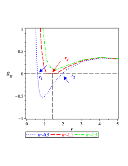
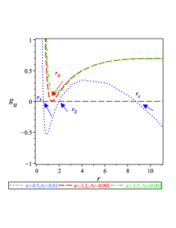
In this section, we will study the thermodynamical properties of the black hole given in (III.1). For this purpose, we remind you of the basic definitions of thermodynamical quantities. First, we depict the behavior of the metric potential in Figure 1 0(a). From Figure 1 0(a), we find that there are two horizons, the inner Cauchy horizon and the outer horizon , when the parameter , these horizons coincides when the dimensional parameter (or more exactly although we have chosen the unit where ), i.e., we have only one horizon which is called the degenerate horizon, , and when , there appears the naked singularity. Finally, we stress that although does not equal to , they have the same Killing and event horizons, that is, when , we find and vice versa.
The Hawking temperature is defined as Sheykhi:2012zz ; Sheykhi:2010zz ; Hendi:2010gq ; Sheykhi:2009pf ; Wang:2018xhw ; Zakria:2018gsf ,
| (42) |
Moreover, the Hawking entropy of the outer horizon is given by
| (43) |
Here is the area of the outer horizon.
The local energy has the following form Cognola:2011nj ; Sheykhi:2012zz ; Sheykhi:2010zz ; Hendi:2010gq ; Sheykhi:2009pf ; Zheng:2018fyn ,
| (44) |
Using the above thermodynamical quantities, we define the Gibbs free energy as follows Zheng:2018fyn ; Kim:2012cma ,
| (45) |
IV.1 The thermodynamics of the black hole solution (III.1)
The black hole solution given by Eq. (III.1) is characterized by its mass , the dimensional parameter , and the electric and magnetic charges and . We stress that the dimensional parameter cannot vanish and therefore we cannot recover the Reissner-Nordström solution in any limit. However, when we set the electric and magnetic field equal to zero and then set , we can recover the Schwarzschild solution which corresponds to general relativity. To find the horizon radii of the black hole (III.1), we solve the equation but we keep the order of up to for an approximation. Under the approximation, the equation has five roots, two of them are real and the other three are pure imaginary. It is difficult to find the analytic forms of these roots easy but the asymptotic forms of the real roots are drawn numerically in Figure 1 0(a). From Figure 1 0(a), we find that there are surely two horizons where .
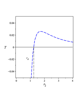

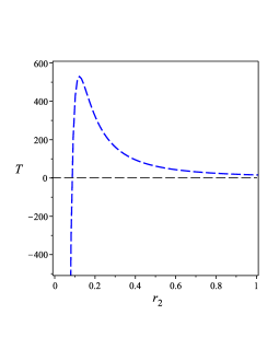
Using Eq. (42), we calculate the Hawking temperature and obtain
| (46) |
The behavior of the temperature given by Eq. (46) is depicted in Figure 1 0(b), which shows that as far as . Figure 1 0(b) indicates that temperature vanishes when . Moreover, when , the temperature becomes negative, and an ultracold black hole is constructed but because there appears a naked singularity, the case could be prohibited by cosmic censorship, that is, the space-time with the naked singularity could not be generated by the collapse of the matters. On the other hand, Davies Davies:1977bgr claimed that there is no concrete reason from the view of thermodynamical effects to stop black hole temperature to take negative values or to create a naked singularity. Figure 1 0(b) seems to support Davies’ argument at region.
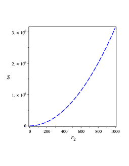
By using Eq. (43), we obtain the entropy of black hole (III.1) as follows,
| (47) |
The behavior of the entropy given by Eq. (47) is depicted in Figure 1 0(c) which indicates that is surely positive and an increasing function of .
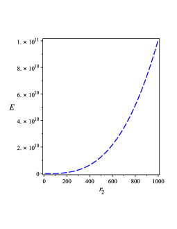
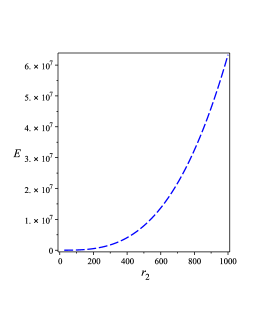
From Eq. (44), we find that the quasi-local energy takes the following form,
| (48) |
The behaviors of the quasi-local energies are shown in Figure 1 0(d) which also shows that is also positive and an increasing function of . Finally, we use Eqs. (46), (47), and (IV.1) in Eq. (45) to calculate the Gibbs free energies and obtain
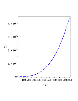
| (49) |
The behavior of this free energy is depicted in Figure 1 0(e) which shows that is positive and an increasing function of , again.
IV.2 Thermodynamics of multi-horizon black hole (III.1) with negative value of the cosmological constant
In the previous subsection, we studied a black hole solution with two horizons where the cosmological constant is positive. In this subsection, we study the same black hole solution but with a negative cosmological constant which generates a cosmological horizon and we obtain the black hole solution with three horizons. The solution is also characterized by the mass , the parameter , and the electric and magnetic charges and . When is negative, the metric components and take the following forms,
| (50) |
When the electric charge , the magnetic charge , and the parameter vanish, the space-time reduces to the Schwarzschild AdS space-time in Einstein’s general relativity. The behavior of in the black hole geometry (IV.2) is drawn in Figure 2 1(a). From Figure 2 1(a), we find that there appear three horizons in general, where in Eq. (IV.2) Wang:2018xhw . Although there are five roots in the equation , three of them are real but the others are imaginary. The expressions of these real roots are lengthy, however, their behaviors are numerically drawn in Figure 2 1(a). From the Figure, we find that the degenerate horizon for the metric potential given by Eq. (IV.2) appears for specific values for , which corresponds to the Nariai black hole.
Using Eq. (42), we obtain the Hawking temperature of the black hole (IV.2) as given by Eq. (46), whose behavior is shown in Figure 2 1(b), which shows that as long as . Figure 2 1(b) also shows that at . When , and an ultracold black hole might be formed.
By using Eq. (44), we draw the quasi-local energy in Figure 2 1(c). The Figure tells that the quasi-local energy is positive and an increasing function of . Finally, using Eqs. (46), (47), and (IV.1) in Eq. (45), we find the Gibbs free energies. The behaviors of these free energies are shown in Figure 2 1(d), which tells us the free energy is positive and an increasing function of , again.
IV.3 First law of thermodynamics in the black holes (III.1) and (IV.2)
It could be interesting to examine if the first law for the black hole geometry (III.1) could be verified. The first law should have the following form even in the gravity Zheng:2018fyn ,
| (51) |
where is the quasi-local energy, is the Bekenstein-Hawking entropy, is the Hawking temperature, is the radial component of the stress-energy tensor that serves as a thermodynamic pressure , and is the geometric volume. In the framework of the gravity, the pressure can be defined as Zheng:2018fyn
| (52) |
For the space-time (III.1), if we neglect , we obtain
| (53) |
By substituting the equations in (IV.3) into (51), we have verified the first law of thermodynamics for the black hole (III.1). Furthermore, by repeating the same procedure for the black hole (IV.2), we verify the first law of thermodynamics, again
V The stability of the black holes
In order to check the stability of the above black hole solutions given by Eqs. (III.1) and (IV.2), we rewrite the action Eq. (2) of the gravity in the scalar-tensor form
| (54) |
where is a scalar field coupled to the Ricci scalar and is the potential (see Capozziello:2011et ; DeFelice:2011ka for details). To discuss the perturbation, we assume that the background is given by the spherically symmetric metric as follows,
| (55) |
Here we denote the background metric by . We check the stability of the black hole solutions, (III.1) and (IV.2), by using the linear perturbations. Moreover, we are going to investigate the value of the propagation speed of the parity-odd perturbation. For the action (54), the background equations have the following forms,
| (56) |
where ′ means the differentiation w.r.t. the radial coordinate, .
V.1 Regge-Wheeler-Zerilli formulation
Following Regge, Wheeler Regge:1957td , and Zerilli Zerilli:1970se , we decompose the perturbed metric by using the decomposition under the two-dimensional rotations. This decomposition is familiar in the perturbations of the Schwarzschild black hole solution in general relativity.
We consider the perturbation of around the background metric , as follows,
| (58) |
Here corresponds to the perturbation and we assume the perturbed quantities to be much smaller than the background, i.e., . Under the two-dimension rotations, , and transform as scalar with spin 0 while and transform as vector with spin 1 and transforms as a tensor with spin 2. Any function including and can be expanded by the spherical harmonics ,
| (59) |
The spherical harmonics satisfies the following equation,
| (60) |
Here is the Laplacian on the two-dimensional unit sphere whose metric is given by . Additionally, the vector can decompose into two parts, that is, the gradient part and the rotational part by using two scalar functions and , as follows,
| (61) |
where is the covariant derivative with respect to the metric and
| (62) |
Here is a second-order skew-symmetric tensor with and .
For , which is a symmetric tensor, can be decomposed as
| (63) |
Here , , and are three scalar functions. Because has three independent components that describe by , we can decompose the tensor to , , and . to decompose . The importance of this decomposition is that in the linearized forms of motion, parity odd-type and parity even-type perturbations are completely decoupled. Note , , are parity-even and therefore they are real scalars but and are parity-odd and pseudo scalars.
In the next subsection, we will study the odd-type perturbations.
V.2 Perturbations with respect to odd-modes
In the Regge-Wheeler formalism, the odd-type metric perturbations have the following form,
| (64) |
By using the gauge transformation , one can choose some of the components in the metric perturbations to vanish. We now use the following transformation of the odd-type perturbation,
| (65) |
and we choose so that vanishes, which is called the Regge-Wheeler gauge. By using the gauge condition, the action of odd modes becomes Regge:1957td
| (66) |
where . We should note that the action (66) does not include the derivative of concerning time, that is , and therefore is not a dynamical degree of freedom. We rewrite in Eq. (66) as in Regge:1957td ; Zerilli:1970se ,
| (67) |
By using the Lagrange multiplier , Eq. (67) can be rewritten as,
| (68) |
By the variation of the action corresponding to Eq. (68) with respect to and , we obtain the equations, which can be solved with respect to and as follows,
| (69) | ||||
| (70) |
Eq. (69) tells that the dynamical degree of the freedom of is transferred to and we can regard as a dynamical field instead of Because is also given in terms of the dynamical field by Eq. (70), by deleting and by using Eqs. (69) and (70) in the action (68), we obtain
| (71) |
where
| (72) |
and
| (73) |
By the coefficient of in the action Eq. (71), we find the condition for the absence of ghosts
| (74) |
Thus, the solutions for and therefore and , which proportional to , when and are large, the radial dispersion relation is given as
| (75) |
Therefore, the radial speed reads
| (76) |
where is the radial tortoise coordinate, defined by and is the proper time, .
We did not investigate the perturbation for the parity-even modes but as in the standard gravity, the modes could correspond to the propagation of the standard spin-two gravitational wave and the spin-zero scalar mode which is specific to the gravity.
VI Discussion and conclusions
Static space-time with spherical symmetry gives an important application for black hole physics Chakraborty:2016lxo . Especially in the case of , by using a specific form of , many spherically symmetric solutions have been derived Nashed:2019tuk ; Elizalde:2020icc ; Nashed:2018oaf ; Nashed:2018efg ; Nashed:2018piz . In this study, we considered a static and spherically symmetric space-time including the case of and we did not assume any specific form of the gravity theory.
First, we stress the following facts:
-
1.
We separated the expression of on one side using the trace of the equation of motions of with electromagnetic fields.
-
2.
By using Eq. (8), we obtained the equation of motions for gravity coupled with electromagnetic fields. The equation involves the first derivative of concerning the Ricci scalar, , i.e., but does not invole itself. By using the equation in the space-time given by Eq. (9) and with electromagnetic fields, we derived the non-linear differential equations which controlled this system. We have solved this system exactly in both cases of and .
-
(a)
When , we have shown that must be a constant, which tells that the Ricci scalar is constant but the electromagnetic field is non-trivial. In this case, the solution coincides with that in Nashed:2019tuk ; Elizalde:2020icc ; Nashed:2018oaf ; Nashed:2018efg ; Nashed:2018piz .
-
(b)
For the case , by assuming have a specific form, i.e., , we solved the system of the non-linear field equations exactly and obtained a solution for the metric and the electric and magnetic fields. We have shown that the Ricci scalar is not a constant and by using the form of the obtained Ricci scalar, we found the expression of in a form of power expansion concerning the Ricci scalar. The main feature in the case is that the solution cannot reproduce the Reissner-Nordström metric of general relativity in any limit. This means that the obtained black hole solution is a new charged exact solution in gravity theory. If the electromagnetic fields and the parameter vanish, we recover the Schwarzschild space-time. Due to the complicated forms of the metric, we have considered their asymptotic forms when the radial coordinate is large, and we have shown that they asymptotically approach AdS/dS space-time. In spite that the field equations of with electromagnetic fields did not involve a cosmological constant, the metric asymptotically approaches AdS/dS which means that acts as a cosmological constant. This effective cosmological constant played an important role in the study of horizons. We have shown that when the effective cosmological constant has a positive value, we obtain two horizons and when the effective cosmological constant is negative, we obtain a black hole with three horizons. In Jaime:2010kn , it has been shown that the conditions for the absence of the ghost is given by and . It is important to stress that our black hole solution in Eq. (III.1) also satisfies the above two conditions.
-
(a)
The Birkhoff theorem has been studied in the frame of the gravity theory Riegert:1984zz . The problem of the Birkhoff theorem in the gravity has been studied by several authors trying to explain if it is valid or not Sotiriou:2011dz ; Sebastiani:2010kv ; PerezBergliaffa:2011gj ; Gao:2016rdu ; Amirabi:2015aya ; Calza:2018ohl ; Oliva:2011xu ; Capozziello:2011wg . The present study did not assume any approximation or conformal transformation to obtain the exact black hole solution (III.1) but the results obtained in this study ensure that the Birkhoff theorem is not true for gravity theories Xavier:2020ulw . It is known that Birkhoff’s theorem is true in general relativity because of the non-existence of zero spin modes in the linear form of the field equations. When the zero spin mode is absent, the spherically symmetric space-time does not couple to higher-spin excitations Misner:1973prb ; Riegert:1984zz . Thus, in the frame of gravity theory, the differential equation verified by the Ricci scalar, , is the source of zero spin modes. Therefore, a non-dependence between the Ricci scalar and the metric, in general, yields the non-validity of the Birkhoff theorem in . This is the case of the exact solution given by Eq. (III.1) which yields a dynamical value of the Ricci scalar .
Moreover, we investigated the inherent physics of the black hole (III.1) by evaluating its scalar invariants given by the squares of the curvatures and showed all its behavior up to the leading order as . These behaviors do not coincide with those in the Reissner-Nordström black hole which yields the leading order of the Kretschmann scalar as and the Ricci tensor squared and . This shows clearly that the singularity of the black hole (III.1) for the Kretschmann scalar is much milder than the black hole of general relativity. We stress that this merit is generated because of the contribution from the higher-order curvature of , i.e., the dimensional parameter .
To clarify the physical properties of the obtained black hole, we calculated some thermodynamical quantities like the entropy, the Hawking temperature, the quasi-local energy, and the Gibbs energy for the case with the effective positive cosmological constant. We have shown that all thermodynamical quantities are consistent with what is presented in the previous literature. Mainly, we have shown that the temperature relies on the radius horizon . When is less than the degenerate horizon, we obtained a negative temperature and the contrary is valid. We did the same calculations when the effective cosmological constant takes a negative value. We have found that the degenerate horizons have an essential role to make the temperature takes a positive value. At the same time, we proved that the black hole verified the first law of thermodynamics.
Another test to examine the black hole (III.1) was the study of its stability. For this purpose, we rewrote the Lagrangian of the gravity by using a scalar field that is coupled with the Ricci scalar-tensor. By investigating the odd-type modes in the perturbation, we have obtained the gradient instability condition and the speed of the radial propagation in the parity-odd mode of the perturbation and find that the speed is equal to unity, that is the speed of light, for black holes (III.1) and (IV.2).
Finally, we stress that the black hole solutions in Eq. (III.1) and (IV.2) are not general solution of the gravity. The reason for this is the fact that in this paper, we have supposed that to obtain the black hole (III.1) and (IV.2). Maybe if we assume another form of , we will obtain another new black hole which will be different from the black hole given by Eq. (III.1) and (IV.2). Moreover, there could be any analytic spherically symmetric interior solution can be derived from the field Eq. (8) following the procedure done in Nashed:2022yfc .
References
- (1) S. Capozziello, Int. J. Mod. Phys. D 11 (2002), 483-492 doi:10.1142/S0218271802002025 [arXiv:gr-qc/0201033 [gr-qc]].
- (2) S. Capozziello, V. F. Cardone, S. Carloni and A. Troisi, Int. J. Mod. Phys. D 12 (2003), 1969-1982 doi:10.1142/S0218271803004407 [arXiv:astro-ph/0307018 [astro-ph]].
- (3) S. M. Carroll, V. Duvvuri, M. Trodden and M. S. Turner, Phys. Rev. D 70 (2004), 043528 doi:10.1103/PhysRevD.70.043528 [arXiv:astro-ph/0306438 [astro-ph]].
- (4) S. Nojiri and S. D. Odintsov, Phys. Rev. D 68 (2003), 123512 doi:10.1103/PhysRevD.68.123512 [arXiv:hep-th/0307288 [hep-th]].
- (5) W. Hu and I. Sawicki, Phys. Rev. D 76 (2007), 064004 doi:10.1103/PhysRevD.76.064004 [arXiv:0705.1158 [astro-ph]].
- (6) A. A. Starobinsky, JETP Lett. 86 (2007), 157-163 doi:10.1134/S0021364007150027 [arXiv:0706.2041 [astro-ph]].
- (7) S. Nojiri and S. D. Odintsov, eConf C0602061 (2006), 06 doi:10.1142/S0219887807001928 [arXiv:hep-th/0601213 [hep-th]].
- (8) E. J. Copeland, M. Sami and S. Tsujikawa, Int. J. Mod. Phys. D 15 (2006), 1753-1936 doi:10.1142/S021827180600942X [arXiv:hep-th/0603057 [hep-th]].
- (9) T. P. Sotiriou and V. Faraoni, Rev. Mod. Phys. 82 (2010), 451-497 doi:10.1103/RevModPhys.82.451 [arXiv:0805.1726 [gr-qc]].
- (10) S. Nojiri and S. D. Odintsov, Phys. Rept. 505 (2011), 59-144 doi:10.1016/j.physrep.2011.04.001 [arXiv:1011.0544 [gr-qc]].
- (11) S. Capozziello and M. De Laurentis, Phys. Rept. 509 (2011), 167-321 doi:10.1016/j.physrep.2011.09.003 [arXiv:1108.6266 [gr-qc]].
- (12) S. Nojiri, S. D. Odintsov and V. K. Oikonomou, Phys. Rept. 692 (2017), 1-104 doi:10.1016/j.physrep.2017.06.001 [arXiv:1705.11098 [gr-qc]].
- (13) T. Clifton, P. G. Ferreira, A. Padilla and C. Skordis, Phys. Rept. 513 (2012), 1-189 doi:10.1016/j.physrep.2012.01.001 [arXiv:1106.2476 [astro-ph.CO]].
- (14) R. Gregory, S. Kanno and J. Soda, JHEP 10 (2009), 010 doi:10.1088/1126-6708/2009/10/010 [arXiv:0907.3203 [hep-th]].
- (15) X. M. Kuang, E. Papantonopoulos, G. Siopsis and B. Wang, Phys. Rev. D 88 (2013), 086008 doi:10.1103/PhysRevD.88.086008 [arXiv:1303.2575 [hep-th]].
- (16) M. Gasperini, Phys. Rev. D 56 (1997), 4815-4823 doi:10.1103/PhysRevD.56.4815 [arXiv:gr-qc/9704045 [gr-qc]].
- (17) S. Hansraj, M. Govender, L. Moodly and K. N. Singh, Phys. Rev. D 105 (2022) no.4, 044030 doi:10.1103/PhysRevD.105.044030 [arXiv:2003.04568 [gr-qc]].
- (18) G. Cognola, E. Elizalde, S. Nojiri, S. D. Odintsov, L. Sebastiani and S. Zerbini, Phys. Rev. D 77 (2008), 046009 doi:10.1103/PhysRevD.77.046009 [arXiv:0712.4017 [hep-th]].
- (19) L. Pogosian and A. Silvestri, Phys. Rev. D 77 (2008), 023503 [erratum: Phys. Rev. D 81 (2010), 049901] doi:10.1103/PhysRevD.77.023503 [arXiv:0709.0296 [astro-ph]].
- (20) P. Zhang, Phys. Rev. D 73 (2006), 123504 doi:10.1103/PhysRevD.73.123504 [arXiv:astro-ph/0511218 [astro-ph]].
- (21) B. Li and J. D. Barrow, Phys. Rev. D 75 (2007), 084010 doi:10.1103/PhysRevD.75.084010 [arXiv:gr-qc/0701111 [gr-qc]].
- (22) Y. S. Song, H. Peiris and W. Hu, Phys. Rev. D 76 (2007), 063517 doi:10.1103/PhysRevD.76.063517 [arXiv:0706.2399 [astro-ph]].
- (23) S. Nojiri and S. D. Odintsov, Phys. Rev. D 77 (2008), 026007 doi:10.1103/PhysRevD.77.026007 [arXiv:0710.1738 [hep-th]].
- (24) S. Nojiri and S. D. Odintsov, Phys. Lett. B 657 (2007), 238-245 doi:10.1016/j.physletb.2007.10.027 [arXiv:0707.1941 [hep-th]].
- (25) S. Capozziello, C. A. Mantica and L. G. Molinari, Int. J. Geom. Meth. Mod. Phys. 16 (2018) no.01, 1950008 doi:10.1142/S0219887819500087 [arXiv:1810.03204 [gr-qc]].
- (26) J. Vainio and I. Vilja, Gen. Rel. Grav. 49 (2017) no.8, 99 doi:10.1007/s10714-017-2262-3 [arXiv:1603.09551 [astro-ph.CO]].
- (27) K. S. Stelle, Phys. Rev. D 16 (1977), 953-969 doi:10.1103/PhysRevD.16.953
- (28) M. Ostrogradsky, Mem. Acad. St. Petersbourg 6 (1850) no.4, 385-517
- (29) R. P. Woodard, Lect. Notes Phys. 720 (2007), 403-433 doi:10.1007/978-3-540-71013-4_14 [arXiv:astro-ph/0601672 [astro-ph]].
- (30) T. Multamaki and I. Vilja, Phys. Rev. D 74 (2006), 064022 doi:10.1103/Multamaki:2006zb [arXiv:astro-ph/0606373 [astro-ph]].
- (31) A. de la Cruz-Dombriz, A. Dobado and A. L. Maroto, Phys. Rev. D 80 (2009), 124011 [erratum: Phys. Rev. D 83 (2011), 029903] doi:10.1103/PhysRevD.80.124011 [arXiv:0907.3872 [gr-qc]].
- (32) S. H. Hendi and D. Momeni, Eur. Phys. J. C 71 (2011), 1823 doi:10.1140/epjc/s10052-011-1823-y [arXiv:1201.0061 [gr-qc]].
- (33) G. G. L. Nashed, Phys. Lett. B 815 (2021), 136133 doi:10.1016/j.physletb.2021.136133 [arXiv:2102.11722 [gr-qc]].
- (34) G. L. L. Nashed and S. Nojiri, JCAP 11 (2021) no.11, 007 doi:10.1088/1475-7516/2021/11/007 [arXiv:2109.02638 [gr-qc]].
- (35) G. G. L. Nashed and S. Nojiri, Phys. Rev. D 104 (2021) no.12, 124054 doi:10.1103/PhysRevD.104.124054 [arXiv:2103.02382 [gr-qc]].
- (36) G. G. L. Nashed, Phys. Lett. B 812 (2021), 136012 doi:10.1016/j.physletb.2020.136012 [arXiv:2101.02205 [gr-qc]].
- (37) G. G. L. Nashed and S. Nojiri, Phys. Rev. D 102 (2020), 124022 doi:10.1103/PhysRevD.102.124022 [arXiv:2012.05711 [gr-qc]].
- (38) G. G. L. Nashed and E. N. Saridakis, Phys. Rev. D 102 (2020) no.12, 124072 doi:10.1103/PhysRevD.102.124072 [arXiv:2010.10422 [gr-qc]].
- (39) G. G. L. Nashed and S. Nojiri, Phys. Lett. B 820 (2021), 136475 doi:10.1016/j.physletb.2021.136475 [arXiv:2010.04701 [hep-th]].
- (40) Z. Y. Tang, B. Wang and E. Papantonopoulos, Eur. Phys. J. C 81 (2021) no.4, 346 doi:10.1140/epjc/s10052-021-09122-8 [arXiv:1911.06988 [gr-qc]].
- (41) G. G. L. Nashed, Eur. Phys. J. Plus 133 (2018) no.1, 18 doi:10.1140/epjp/i2018-11849-7
- (42) G. G. L. Nashed, Int. J. Mod. Phys. D 27 (2018) no.7, 1850074 doi:10.1142/S0218271818500748
- (43) G. G. L. Nashed, Adv. High Energy Phys. 2018 (2018), 7323574 doi:10.1155/2018/7323574
- (44) L. Sebastiani and S. Zerbini, Eur. Phys. J. C 71 (2011), 1591 doi:10.1140/epjc/s10052-011-1591-8 [arXiv:1012.5230 [gr-qc]].
- (45) S. H. Hendi, B. Eslam Panah and R. Saffari, Int. J. Mod. Phys. D 23 (2014) no.11, 1450088 doi:10.1142/S0218271814500886 [arXiv:1408.5570 [hep-th]].
- (46) T. Multamaki and I. Vilja, Phys. Rev. D 76 (2007), 064021 doi:10.1103/PhysRevD.76.064021 [arXiv:astro-ph/0612775 [astro-ph]].
- (47) G. G. L. Nashed and K. Bamba, PTEP 2020 (2020) no.4, 043E05 doi:10.1093/ptep/ptaa025 [arXiv:1902.08020 [gr-qc]].
- (48) G. G. L. Nashed and S. Capozziello, Phys. Rev. D 99 (2019) no.10, 104018 doi:10.1103/PhysRevD.99.104018 [arXiv:1902.06783 [gr-qc]].
- (49) S. C. Jaryal and A. Chatterjee, Eur. Phys. J. C 81 (2021) no.4, 273 doi:10.1140/epjc/s10052-021-09079-8 [arXiv:2102.08717 [gr-qc]].
- (50) E. F. Eiroa and G. Figueroa-Aguirre, Phys. Rev. D 103 (2021) no.4, 044011 doi:10.1103/PhysRevD.103.044011 [arXiv:2011.14952 [gr-qc]].
- (51) Z. Y. Tang, B. Wang, T. Karakasis and E. Papantonopoulos, Phys. Rev. D 104 (2021) no.6, 064017 doi:10.1103/PhysRevD.104.064017 [arXiv:2008.13318 [gr-qc]].
- (52) T. Karakasis, E. Papantonopoulos, Z. Y. Tang and B. Wang, Phys. Rev. D 103 (2021) no.6, 064063 doi:10.1103/PhysRevD.103.064063 [arXiv:2101.06410 [gr-qc]].
- (53) T. Karakasis, E. Papantonopoulos, Z. Y. Tang and B. Wang, Eur. Phys. J. C 81 (2021) no.10, 897 doi:10.1140/epjc/s10052-021-09717-1 [arXiv:2103.14141 [gr-qc]].
- (54) S. Pi, Y. l. Zhang, Q. G. Huang and M. Sasaki, JCAP 05 (2018), 042 doi:10.1088/1475-7516/2018/05/042 [arXiv:1712.09896 [astro-ph.CO]].
- (55) A. de la Cruz-Dombriz, E. Elizalde, S. D. Odintsov and D. Sáez-Gómez, JCAP 05 (2016), 060 doi:10.1088/1475-7516/2016/05/060 [arXiv:1603.05537 [gr-qc]].
- (56) S. Capozziello, A. Stabile and A. Troisi, Class. Quant. Grav. 24 (2007), 2153-2166 doi:10.1088/0264-9381/24/8/013 [arXiv:gr-qc/0703067 [gr-qc]].
- (57) S. Capozziello, N. Frusciante and D. Vernieri, Gen. Rel. Grav. 44 (2012), 1881-1891 doi:10.1007/s10714-012-1367-y [arXiv:1204.4650 [gr-qc]].
- (58) S. Capozziello, M. De laurentis and A. Stabile, Class. Quant. Grav. 27 (2010), 165008 doi:10.1088/0264-9381/27/16/165008 [arXiv:0912.5286 [gr-qc]].
- (59) E. Elizalde, G. G. L. Nashed, S. Nojiri and S. D. Odintsov, Eur. Phys. J. C 80 (2020) no.2, 109 doi:10.1140/epjc/s10052-020-7686-3 [arXiv:2001.11357 [gr-qc]].
- (60) G. G. L. Nashed, W. El Hanafy, S. D. Odintsov and V. K. Oikonomou, Int. J. Mod. Phys. D 29 (2020) no.13, 2050090 doi:10.1142/S021827182050090X [arXiv:1912.03897 [gr-qc]].
- (61) J. Sultana and D. Kazanas, Gen. Rel. Grav. 50 (2018) no.11, 137 doi:10.1007/s10714-018-2463-4 [arXiv:1810.02915 [gr-qc]].
- (62) P. Cañate, Class. Quant. Grav. 35 (2018) no.2, 025018 doi:10.1088/1361-6382/aa8e2e
- (63) S. Yu, C. Gao and M. Liu, Res. Astron. Astrophys. 18 (2018) no.12, 157 doi:10.1088/1674-4527/18/12/157 [arXiv:1711.04064 [gr-qc]].
- (64) P. Cañate, L. G. Jaime and M. Salgado, Class. Quant. Grav. 33 (2016) no.15, 155005 doi:10.1088/0264-9381/33/15/155005 [arXiv:1509.01664 [gr-qc]].
- (65) A. Kehagias, C. Kounnas, D. Lüst and A. Riotto, JHEP 05 (2015), 143 doi:10.1007/JHEP05(2015)143 [arXiv:1502.04192 [hep-th]].
- (66) W. Nelson, Phys. Rev. D 82 (2010), 104026 doi:10.1103/PhysRevD.82.104026 [arXiv:1010.3986 [gr-qc]].
- (67) W. X. Feng, C. Q. Geng, W. F. Kao and L. W. Luo, Int. J. Mod. Phys. D 27 (2017) no.01, 1750186 doi:10.1142/S0218271817501863 [arXiv:1702.05936 [gr-qc]].
- (68) M. Aparicio Resco, Á. de la Cruz-Dombriz, F. J. Llanes Estrada and V. Zapatero Castrillo, Phys. Dark Univ. 13 (2016), 147-161 doi:10.1016/j.dark.2016.07.001 [arXiv:1602.03880 [gr-qc]].
- (69) S. Capozziello, M. De Laurentis, R. Farinelli and S. D. Odintsov, Phys. Rev. D 93 (2016) no.2, 023501 doi:10.1103/PhysRevD.93.023501 [arXiv:1509.04163 [gr-qc]].
- (70) K. V. Staykov, D. Popchev, D. D. Doneva and S. S. Yazadjiev, Eur. Phys. J. C 78 (2018) no.7, 586 doi:10.1140/epjc/s10052-018-6064-x [arXiv:1805.07818 [gr-qc]].
- (71) D. D. Doneva and S. S. Yazadjiev, JCAP 11 (2016), 019 doi:10.1088/1475-7516/2016/11/019 [arXiv:1607.03299 [gr-qc]].
- (72) S. S. Yazadjiev, D. D. Doneva and D. Popchev, Phys. Rev. D 93 (2016) no.8, 084038 doi:10.1103/PhysRevD.93.084038 [arXiv:1602.04766 [gr-qc]].
- (73) S. S. Yazadjiev, D. D. Doneva and K. D. Kokkotas, Phys. Rev. D 91 (2015) no.8, 084018 doi:10.1103/PhysRevD.91.084018 [arXiv:1501.04591 [gr-qc]].
- (74) S. S. Yazadjiev, D. D. Doneva, K. D. Kokkotas and K. V. Staykov, JCAP 06 (2014), 003 doi:10.1088/1475-7516/2014/06/003 [arXiv:1402.4469 [gr-qc]].
- (75) A. Ganguly, R. Gannouji, R. Goswami and S. Ray, Phys. Rev. D 89 (2014) no.6, 064019 doi:10.1103/PhysRevD.89.064019 [arXiv:1309.3279 [gr-qc]].
- (76) A. V. Astashenok, S. Capozziello and S. D. Odintsov, JCAP 12 (2013), 040 doi:10.1088/1475-7516/2013/12/040 [arXiv:1309.1978 [gr-qc]].
- (77) M. Orellana, F. Garcia, F. A. Teppa Pannia and G. E. Romero, Gen. Rel. Grav. 45 (2013), 771-783 doi:10.1007/s10714-013-1501-5 [arXiv:1301.5189 [astro-ph.CO]].
- (78) A. S. Arapoglu, C. Deliduman and K. Y. Eksi, JCAP 07 (2011), 020 doi:10.1088/1475-7516/2011/07/020 [arXiv:1003.3179 [gr-qc]].
- (79) A. Cooney, S. DeDeo and D. Psaltis, Phys. Rev. D 82 (2010), 064033 doi:10.1103/PhysRevD.82.064033 [arXiv:0910.5480 [astro-ph.HE]].
- (80) C. Brans and R. H. Dicke, Phys. Rev. 124 (1961), 925-935 doi:10.1103/Brans:1961sx
- (81) T. Chiba, Phys. Lett. B 575 (2003), 1-3 doi:10.1016/j.physletb.2003.09.033 [arXiv:astro-ph/0307338 [astro-ph]].
- (82) J. O’Hanlon, Phys. Rev. Lett. 29 (1972), 137-138 doi:10.1103/OHanlon:1972xqa
- (83) S. Chakraborty and S. SenGupta, Eur. Phys. J. C 77 (2017) no.8, 573 doi:10.1140/epjc/s10052-017-5138-5 [arXiv:1701.01032 [gr-qc]].
- (84) S. Chakraborty and S. SenGupta, Eur. Phys. J. C 76 (2016) no.10, 552 doi:10.1140/epjc/s10052-016-4394-0 [arXiv:1604.05301 [gr-qc]].
- (85) H. A. Buchdahl, Mon. Not. Roy. Astron. Soc. 150 (1970), 1
- (86) G. Cognola, E. Elizalde, S. Nojiri, S. D. Odintsov and S. Zerbini, JCAP 02 (2005), 010 doi:10.1088/1475-7516/2005/02/010 [arXiv:hep-th/0501096 [hep-th]].
- (87) T. Koivisto and H. Kurki-Suonio, Class. Quant. Grav. 23 (2006), 2355-2369 doi:10.1088/0264-9381/23/7/009 [arXiv:astro-ph/0509422 [astro-ph]].
- (88) C. W. Misner, K. S. Thorne and J. A. Wheeler,
- (89) A. Sheykhi, Phys. Rev. D 86 (2012), 024013 doi:10.1103/Sheykhi:2012zz [arXiv:1209.2960 [hep-th]].
- (90) A. Sheykhi, Eur. Phys. J. C 69 (2010), 265-269 doi:10.1140/epjc/s10052-010-1372-9 [arXiv:1012.0383 [hep-th]].
- (91) S. H. Hendi, A. Sheykhi and M. H. Dehghani, Eur. Phys. J. C 70 (2010), 703-712 doi:10.1140/epjc/s10052-010-1483-3 [arXiv:1002.0202 [hep-th]].
- (92) A. Sheykhi, M. H. Dehghani and S. H. Hendi, Phys. Rev. D 81 (2010), 084040 doi:10.1103/Sheykhi:2009pf [arXiv:0912.4199 [hep-th]].
- (93) Y. Q. Wang, Y. X. Liu and S. W. Wei, Phys. Rev. D 99 (2019) no.6, 064036 doi:10.1103/PhysRevD.99.064036 [arXiv:1811.08795 [gr-qc]].
- (94) A. Zakria and A. Afzal, [arXiv:1808.04361 [hep-th]].
- (95) G. Cognola, O. Gorbunova, L. Sebastiani and S. Zerbini, Phys. Rev. D 84 (2011), 023515 doi:10.1103/Cognola:2011nj [arXiv:1104.2814 [gr-qc]].
- (96) Y. Zheng and R. J. Yang, Eur. Phys. J. C 78 (2018) no.8, 682 doi:10.1140/epjc/s10052-018-6167-4 [arXiv:1806.09858 [gr-qc]].
- (97) W. Kim and Y. Kim, Phys. Lett. B 718 (2012), 687-691 doi:10.1016/j.physletb.2012.11.017 [arXiv:1207.5318 [gr-qc]].
- (98) P. C. W. Davies, Proc. Roy. Soc. Lond. A 353 (1977), 499-521 doi:10.1098/rspa.1977.0047
- (99) A. De Felice, T. Suyama and T. Tanaka, Phys. Rev. D 83 (2011), 104035 doi:10.1103/PhysRevD.83.104035 [arXiv:1102.1521 [gr-qc]].
- (100) T. Regge and J. A. Wheeler, Phys. Rev. 108 (1957), 1063-1069 doi:10.1103/Regge:1957td
- (101) F. J. Zerilli, Phys. Rev. Lett. 24 (1970), 737-738 doi:10.1103/Zerilli:1970se
- (102) S. Chakraborty and S. SenGupta, JCAP 07 (2017), 045 doi:10.1088/1475-7516/2017/07/045 [arXiv:1611.06936 [gr-qc]].
- (103) L. G. Jaime, L. Patino and M. Salgado, Phys. Rev. D 83 (2011), 024039 doi:10.1103/PhysRevD.83.024039 [arXiv:1006.5747 [gr-qc]].
- (104) R. J. Riegert, Phys. Rev. Lett. 53 (1984), 315-318 doi:10.1103/PhysRevLett.53.315
- (105) T. P. Sotiriou and V. Faraoni, Phys. Rev. Lett. 108 (2012), 081103 doi:10.1103/PhysRevLett.108.081103 [arXiv:1109.6324 [gr-qc]].
- (106) S. E. Perez Bergliaffa and Y. E. C. de Oliveira Nunes, Phys. Rev. D 84 (2011), 084006 doi:10.1103/PhysRevD.84.084006 [arXiv:1107.5727 [gr-qc]].
- (107) C. Gao and Y. G. Shen, Gen. Rel. Grav. 48 (2016) no.10, 131 doi:10.1007/s10714-016-2128-0 [arXiv:1602.08164 [gr-qc]].
- (108) Z. Amirabi, M. Halilsoy and S. Habib Mazharimousavi, Eur. Phys. J. C 76 (2016) no.6, 338 doi:10.1140/epjc/s10052-016-4164-z [arXiv:1509.06967 [gr-qc]].
- (109) M. Calzà, M. Rinaldi and L. Sebastiani, Eur. Phys. J. C 78 (2018) no.3, 178 doi:10.1140/epjc/s10052-018-5681-8 [arXiv:1802.00329 [gr-qc]].
- (110) J. Oliva and S. Ray, Class. Quant. Grav. 28 (2011), 175007 doi:10.1088/0264-9381/28/17/175007 [arXiv:1104.1205 [gr-qc]].
- (111) S. Capozziello and D. Saez-Gomez, Annalen Phys. 524 (2012), 279-285 doi:10.1002/andp.201100244 [arXiv:1107.0948 [gr-qc]].
- (112) S. Xavier, J. Mathew and S. Shankaranarayanan, Class. Quant. Grav. 37 (2020) no.22, 225006 doi:10.1088/1361-6382/abbd0f [arXiv:2003.05139 [gr-qc]].
- (113) G. G. L. Nashed and E. N. Saridakis, [arXiv:2206.12256 [gr-qc]].