Black hole binaries and light fields: Gravitational molecules
Abstract
We show that light scalars can form quasibound states around binaries. In the nonrelativistic regime, these states are formally described by the quantum-mechanical Schrödinger equation for a one-electron heteronuclear diatomic molecule. We performed extensive numerical simulations of scalar fields around black hole binaries showing that a scalar structure condenses around the binary – we dub these states “gravitational molecules”. We further show that these are well described by the perturbative, nonrelativistic description.
I Introduction
More than one century after Einstein wrote down the field equations of general relativity, black holes (BHs) remain one of its most outstanding and intriguing predictions. Among all of its features, the inherent simplicity of stationary BHs is possibly the most remarkable one: just two numbers (mass and angular momentum) suffice to fully characterize these objects in vacuum Bekenstein (1972); Robinson (1975); Bekenstein (1997); Chrusciel et al. (2012).
This simplicity and fundamental nature has led to analogies being drawn between BHs in general relativity and the hydrogen atom in quantum mechanics. In fact, in the context of fundamental fields in curved spacetime, BHs do behave as atoms: massive scalar fields can form long-lived states which are, in a certain limit, mathematically described by the nonrelativistic Schrödinger equation for the hydrogen atom Brito et al. (2015a); Detweiler (1980); Arvanitaki and Dubovsky (2011); Baumann et al. (2019a); such states have been dubbed “gravitational atoms” Baumann et al. (2019a).
The horizon of non-spinning BHs acts as a dissipative surface, and hence these scalar states are in general “quasibound”. When the host BH is spinning these configurations may grow via superradiance, extracting a substantial fraction of the BH rotation energy to a bosonic “cloud” in the BH exterior. The process slows the BH spin down and releases monochromatic gravitational waves, giving rise to very particular imprints. These states may form, through a different process, as a consequence of boson star collisions Sanchis-Gual et al. (2020) or collisions between axion stars and BHs Clough et al. (2018). Thus BHs can be used as efficient particle detectors of ultralight fields across a wide range of mass Brito et al. (2015a, b); Yoshino and Kodama (2014). For fine-tuned conditions, the states can become truly bound states, and new BH solutions become possible Herdeiro and Radu (2014).
Black hole binaries were recently shown to have characteristic vibration modes Bernard et al. (2019). Together with the above discussion on gravitational atoms, one is led to ask whether the program can be taken a step further: Does it make sense to talk about “gravitational molecules”? Recent work using effective field theory techniques indicates that quasibound states of light scalars engulfing binaries could exist Wong (2020). We explore this question further here both analytically and numerically, and give a positive answer providing (under certain mild conditions), an equivalence between BH binaries and dihydrogen molecules.
We will study this issue by looking at the dynamics of massive scalar fields in a BH binary (BHB) spacetime. We thus consider a Klein-Gordon scalar, governed by the equation
| (1) |
in a nontrivial background describing a binary—in particular, a BHB. We always neglect backreaction of the field in the spacetime geometry, which in all but extreme situations should be a very accurate approximation. Here, the mass parameter is related to the boson mass .
We use geometric units and a convention for the metric signature throughout.
II Nonrelativistic scalars around binaries
We first explore the problem in a nonrelativistic setting. This means that the spacetime is taken to be weakly curved, and could describe, for instance, two noncompact stars. It also means that the rest mass of the scalar dominates over its kinetic energy.
II.1 Equivalence with dihydrogen molecules
In a nonrelativistic setting, the Klein-Gordon equation around a single BH reduces to the Schrödinger equation Brito et al. (2015a); Arvanitaki and Dubovsky (2011); Baumann et al. (2019a). There is thus a quasibound state structure for scalar fields around a BH which is identical to the spectrum of the hydrogen atom. Let us now consider the nonrelativistic limit of a scalar field around a BHB. To lowest order in a post-Newtonian expansion, the geometry of a binary (including that of a BHB, if we are not interested in near-horizon phenomena) can be written in the form
| (2) |
where
| (3) |
is Newton’s potential. Here, are the individual component masses, and are their position vector. There are higher-order terms which depend on the specifics of the system, and which become relevant for relativistic and strongly gravitating systems, but which do not affect the physics we are interested in.
Using standard nonrelativistic limit procedures, we define the complex field as
| (4) |
Note that the Klein-Gordon field is assumed to be real throughout this work. The field is, in general, complex. Assuming that the binary components are widely separated and that the angular frequency is so small that time-dependent terms in the Newtonian potential can be neglected, the Klein-Gordon equation (1) reduces to the Schrödinger equation
| (5) |
where we neglect the subleading (for weakly gravitating, nonrelativistic systems) terms
We can also recover Eq. (5) via a Lagrangian approach Baumann et al. (2019b).
Equation (5) is written in the lab frame, . It will be useful to write it in the binary rest frame (corotating frame), , which we can do with the usual coordinate transformation
| (6) |
where spans the orbital plane, and is the BHB orbital angular velocity. The frames are related through
| (7) |
Denoting , and remembering that , we can then rewrite Eq. (5) in the corotating frame as
| (8) |
where
| (9) |
and the (time-independent) potential is given by
| (10) |
where is the distance to BH , and are the positions of each BH.
Equation (8) can be treated perturbatively when is small. Let us first consider the unperturbed system,
Since the potential is not time dependent, we can consider the energy eigenstate problem; writing
| (11) |
we then have
| (12) |
Introducing prolate spheroidal coordinates
| (13) |
where is the separation between the two BHs on the axis and , , and , Eq. (12) becomes separable. Using the ansatz
| (14) |
with , we then find
| (15a) | |||
| (15b) | |||
where we define
Here, is a separation constant. and are labeled by three integers , , , characterizing the properties of the solutions of the coupled system. We will focus on bound-state solutions, for which .
It is then easily seen that this gravitational problem is completely equivalent to the quantum-mechanical Schrödinger equation for the electronic energy of a one-electron heteronuclear diatomic molecule. In particular, if we identify , then the equations above are mathematically equivalent to the quantum-mechanical problem (in atomic units), where the nuclei have atomic numbers each and are separated by a fixed distance Burrau (1927); Wilson (1928); Brown and Steiner (1966); Nickel (2011); Leaver (1986). In particular, this system also describes the ionized dihydrogen molecule Burrau (1927); Wilson (1928). We thus have a formal equivalence between two similar systems, that of a molecule governed by electromagnetism and a simple binary system in a Newtonian setting. We will see below that the inclusion of full general-relativistic effects alters this picture only slightly.
| (0,0,0) | ||||
|---|---|---|---|---|
| (1,0,0) | ||||
| (2,0,0) | ||||
| (0,2,0) | ||||
| (1,2,0) | ||||
| (2,2,0) | ||||
Equations (15) are of spheroidal type. The first is an “angular”-type scalar spheroidal equation Leaver (1986); Berti et al. (2006), and it is coupled to the second (radial) equation through the (unknown) energy and separation constant . We have solved this system to find the characteristic energies , with two different methods. We use direct integration of the ordinary differential equations, shooting to the energy; in addition, we used a high-accuracy continued fraction approach to solve the same problem Leaver (1986). Our numerical results for selected values of the separation are shown in Table 1.
II.2 The single black hole limit
At zero separation, we are effectively dealing with one single BH, for which the energy levels are known to high precision. In spherical polar coordinates the eigenfunction is
| (16) | ||||
| (17) |
with being the scalar spherical harmonics and a generalized Laguerre polynomial (it’s a polynomial of order in its argument). Note that is the BHB mass. With these definitions and conventions, the energy eigenvalue is
| (18) |
up to . Higher-order expansions in can be calculated using well-known techniques and are shown in Ref. Baumann et al. (2019a), with a different state label. Notice that we follow the state labeling of Ref. Brito et al. (2015a). The scalar profile of mode decays spatially as and the angular profile is dictated by the corresponding spherical harmonic. The spatial extent of the scalar configuration is defined by the exponential decay, and is of order .
Note that the prolate coordinates [Eq. (13)] are also given by
| (19) |
Defining spherical coordinates such that
one finds, when ,
The relation between quantum numbers is then, in this limit Bates and Reid (1968)
| (20) |
For small separations , our results—shown in Table 1—for the fundamental () mode are compatible with (up to terms of order )
| (21) |
This analytic expansion was derived by Bethe, and in subsequent analytical work for the dihydrogen molecule and generalizations thereof Bethe (1933); Brown and Steiner (1966); Nickel (2011); Bates and Reid (1968); Abramov and Slavyanov (2001); Damburg et al. (1984). Our own numerical results in the limit of small binary separation are in perfect agreement with such expression.
We note that for our numerical simulations shown in Sec. IV, we will use a frame rotated by 90 degrees, which therefore superposes different states. In addition, and more importantly, at finite separation , we can no longer use Eq. (20): a given state in the basis involves, generically, a superposition of all modes in a spherical harmonic decomposition, such as that of Sec. IV.
II.3 Relation with classical closed orbits
Particle analogies of wave equations often play an important role in several physical phenomena. In particular, a lot of BH physics described by wave equations have particle descriptions which helps us to understand the system from a different point of view. For example, BH quasinormal modes (QNMs) can be related to closed null orbits around the BH based on the WKB approximation, where the QNM frequencies can be estimated from the orbital periods Cardoso et al. (2009). Conversely, the existence of closed null orbits around relativistic objects may hint at the possibility of the existence of QNMs Bernard et al. (2019).
We will therefore study the particle analog of the system we have been considering of a massive scalar field around a BHB. As we will now see, this particle description can be derived from the WKB approximation of Schrödinger’s equation and can be applied to states around a general separable spacetime.
In quantum mechanics, it is well known that the first order of the WKB approximation corresponds to the Hamilton-Jacobi equation for a classical particle, and the energy spectrum can be related to the particle motion through the Bohr-Sommerfeld condition Weinberg (2015)111Strictly speaking, the Bohr-Sommerfeld condition is ; however, since we are only interested in its large- limit, we have neglected the term in Eq. (22).
| (22) |
where and are the canonical coordinates and is an integer. The integral is performed over a closed classical orbit which is described by the corresponding Hamilton-Jacobi equation. Since this is derived from the WKB approximation, we can use this relation in the large- limit to estimate the frequency of the bound states of Sec. II.1.
Furthermore, from the classically allowed regions of the Hamilton-Jacobi equation, we can have an idea about the spatial profile of the wave function. Since, as shown in the previous subsection, our system can be described by Schrödinger’s equation, we can apply these arguments to get the relation between (truly) bound states and closed orbits of a massive particle.222These are actual bound states because we are using a Newtonian approximation, and horizons are not present.
Let us then consider the classical motion under Newton’s potential [Eq. (10)], which corresponds to the motion of a massive particle (of mass ) around a BHB, in the binary rest frame. The Lagrangian for the particle is
where are the particle’s coordinates. Using the coordinates , the Hamilton-Jacobi equation reads
| (23) |
where is Hamilton’s principal function. In these coordinates the Hamilton-Jacobi equation is separable; we thus write
and after substituting into Eq. (23), we obtain
| (24) | ||||
where is a separation constant. Comparing with Eq. (15), we see that corresponds to . For classical motion, the right-hand side of Eq. (24) must be positive, and the parameter space where this happens corresponds to the classically allowed region. The topology of this region can change depending on the parameters; for simplicity, we will focus on equal-mass binaries () and on bound states around the binary () with .


Considering first the case, we see from Eq. (24) that is unconstrained (), and the allowed region for is determined from
| (25) |
When , the allowed region for is , and when , the allowed region is . Here, are solutions of the equation :
| (26) |
Therefore, when , the particle motion is an orbit around the binary (see the first and second panels in Fig. 1).
We now focus on the case. The allowed region for is for . Existence of solutions to Eq. (25) then implies that , and the corresponding allowed region for is then (see the third panel in Fig. 1). In this case, the motion is an orbit around each individual BH.
Since the WKB approximation is valid only in the high-frequency limit, we cannot easily apply this classical picture to the states from the previous subsection. We can, however, see that there are two distinct profiles for these states: one corresponding to configurations bound to each individual BH, and another corresponding to a configuration bound to the binary as a whole.
In order to compare the particle picture to the states of the previous subsection, let us discuss the spectrum of these states using the Bohr-Sommerfeld condition Eq. (22). From this condition we immediately see that must be the integer and we further get
| (27a) | ||||
| (27b) | ||||
where and are integers, and the integration limits and are the roots of the expressions inside each square root. Since Eqs. (27) cannot be integrated analytically let us consider the hydrogen atom limit () by fixing and in the equal-mass case (). We obtain the spectrum
These expressions are in good agreement with the spectrum of the hydrogen atom in the large- and large- limit, confirming the validity of this particle picture.
II.4 Corrections induced by orbital motion
Having solved Eq. (8) to zeroth order in , let us now consider, perturbatively, the effect of rotation. The first-order correction in to the unperturbed energy levels that we have just computed is given by the expectation value of the rotation operator for the system in the unperturbed state. In the coordinates this operator takes the form
| (28) |
Since and , we can easily see that the expectation value of this operator in an eigenstate [Eq. (14)] is zero, . This shows that rotation effects only manifest themselves at order and will therefore be neglected.
III Setup for time evolutions
In the previous section we discussed, in a perturbative setup, the nonrelativistic limit of a massive scalar field around a BHB and found molecule-like states which were labeled therein with three parameters . We will now numerically solve the Klein-Gordon equation around a BHB to construct these (quasi)bound states through time evolutions.
III.1 Numerical implementation
For our numerical implementation we ignore the backreaction of the massive scalar field on the BHB spacetime and follow the approach described in Ref. Bernard et al. (2019). In this approach one builds an approximate BHB background metric using the construction outlined in detail in Mundim et al. Mundim et al. (2014) (see also Ref. Johnson-McDaniel et al. (2009) for the equivalent construction used in the context of generating BHB initial data). It is important to mention that for our present construction we turn off the emission of gravitational radiation and therefore always consider binaries with constant separation. We do not turn off scalar radiation; the Klein-Gordon equation is evolved in full generality.
Our approach then consists in using this approximate BHB metric construction and solving the Klein-Gordon equation (1) in this spacetime. We emphasize that this metric, even though it is time-dependent, is prescribed—that is, it is not time-evolved. Our task is then to numerically solve Eq. (1) on a time-dependent background. To do so we write the equation in a first-order form by introducing
| (29) |
where and are the lapse function and shift vector, respectively. The resulting system is numerically evolved with a method of lines approach.
For our numerical evolutions, we use the Einstein Toolkit infrastructure Löffler et al. (2012); Zilhão and Löffler (2013); Babiuc-Hamilton et al. (2019) with Carpet Schnetter et al. (2004); Carpet for mesh refinement capabilities and the multipatch infrastructure Llama Pollney et al. (2011). The scalar field equations are evolved in time by adapting the ScalarEvolve code available in Ref. Witek et al. (2020), which was first used and described in Ref. Cunha et al. (2017). Since the background metric uses harmonic coordinates, in our evolutions we further excise the BH interior with the procedure outlined in Ref. Assumpcao et al. (2018). The overall infrastructure and evolution are essentially the same those used and tested in Ref. Bernard et al. (2019). We employ fourth-order-accurate finite-differencing stencils to approximate spatial derivatives, but there are lower-order elements in the code—in particular the so-called prolongation operation is only second-order accurate in time. Our results are compatible with a convergence order between orders 2 and 3, which is consistent with the overall setup. See Appendix B for further details.
III.2 Initial data
We will evolve two different types of scalar field initial data, which will be referred to as “nonspinning” and “spinning” initial data. The first of these consists of a momentarily static Gaussian profile given by
| (30) |
where and denote the amplitude and width of the Gaussian pulse, respectively.
Secondly, we will evolve configurations which, unlike the previous construction, have angular momentum. These are the “spinning” initial data, for which
| (31) |
with
| (32) | ||||
| (33) |
and the initial configuration for the field can be trivially obtained from Eq. (29). Here, is the amplitude of each mode, which can be freely specified, and is a typical width of the clump. are the standard spherical coordinates around the center of mass of the system. The time dependence in each term introduces angular momentum on the axis. Initial data with negative are corotating with the BHB, while initial data with positive are antirotating.
III.3 Frequency extraction
To analyze our results, we decompose the evolved field at fixed radial distance into spherical harmonics as follows
| (34) |
Note that, since is real, where denotes complex conjugation. We will further Fourier-transform to check its frequency spectra and compare with the results obtained in Sec. II.1. In order to do so, however, we must note that the frequencies computed in Sec. II.1 were computed in the rest frame of the binary, whereas here we will be extracting the data in the lab frame. To compare the data we then need to change frames once again, which can be done as follows:
The Fourier spectra in the lab frame is computed through []
| (35) |
Given that , where are the Legendre polynomials and is the normalization constant, using Eq. (6), we can write
| (36) |
relating the frequencies computed in the lab frame to the ones computed in the comoving frame.
Since in the following section we will be focusing on the real part of the multipolar components let us also write
| (37) |
where and Eq. (36) is used in the last step. To connect with our upcoming results we further need to take the real part of Eq. (37),
where we have used
In conclusion, in the lab frame we expect to see a superposition of frequencies for each mode of the corotating frame.
IV Gravitational molecules
We are now in a position to discuss the evolution of scalar fields on a background describing realistic BHBs. We have evolved a battery of different configurations with the initial data of Eqs. (30) and (31) on background spacetimes described by equal-mass binaries, , for different values of binary separation . In this section we will report on the results obtained with a subset of these runs, summarized in Tables 2 and 3. The numerical convergence for the simulations nonspin2 is discussed in Appendix B. These results, as described below, are in good agreement with the nonrelativistic analysis of Sec. II, and provide strong evidence for the existence and formation of gravitational molecules with scalar fields.
| Run | |||
|---|---|---|---|
| nonspin1 | 60 | 0.5 | 12 |
| nonspin2 | 10 | 0.2 | 25 |
| nonspin3 | 60 | 0.2 | 25 |
| Run | ||||||
|---|---|---|---|---|---|---|
| spin1 | 10 | 0.2 | 25 | 0 | 1 | 0.2 |
| spin2 | 60 | 0.2 | 25 | 0 | 1 | 0.2 |
| spin3 | 60 | 0.2 | 25 | 1 | 0 | 0.2 |
It is useful to keep in mind the different length scales involved in this problem. As we saw in Sec. II.2, the scale of a state around an isolated BH of mass is of order in the small- limit. In a binary of component masses , we thus have scales , and a global scale where the total BHB mass is . If is much smaller than , the quasibound state can be formed around each BH and feels a tidal force from the companion object. On the other hand, if is much larger than , the companion BH strongly disturbs such a state, destroying it. However, as discussed in Sec. II, we can expect that a quasibound state forms around the BHB. Furthermore, if this state around the binary is stable, it should be formed starting from generic initial conditions.
Note also that timescales are important. A light-crossing timescale is of order , whereas an orbital timescale is of order or for binaries separated by or , respectively.


IV.1 quasibound states around individual BHs
Based on the scales above, we expect that for large enough couplings the scale obeys , in which case the scalar cloud localizes around each BH but not around the binary. In other words, we expect that BHs sufficiently far apart can support clouds as if in isolation. To test this, we evolve momentarily static Gaussian initial data, Eq. (30), corresponding to configuration nonspin1 in Table 2. For these parameters, the typical size of the cloud around each BH is , which is smaller than the BH separation. We therefore expect that quasibound states form around each BH and our results confirm this, as shown in Fig. 2. As can be seen, localized structures are apparent with the dominant mode being an state around each individual BH. Our results show that these configurations remain localized to the binary with negligible variation in its shape and topology for thousands of dynamical timescales, with only a slight variation in amplitude, hence qualifying as true quasibound states.
IV.2 Global quasibound states from evolution of static initial data
We will now discuss molecular-like structures—i.e., scalar clouds around BHBs. We focus on BH separations , and we fix the mass of the scalar field to . This corresponds to configurations nonspin2 and nonspin3, respectively. The scales are such that now the size of the quasibound states, if present, would encompass the binary when . We will see that even for such global states exist.


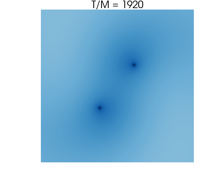


The evolution of these configurations is shown in Fig. 3. Perhaps the most evident aspect of these simulations is that there is a persistent structure, a cloud or quasibound state of scalar field around the binary for relatively long time. In the context of Fig. 3, the evolution timescale is large enough that the binary performed over ten periods for configuration nonspin2 and two periods for configuration nonspin3. This timescale is orders of magnitude larger than the free fall time, and yet the scalar structure persists throughout the evolution.
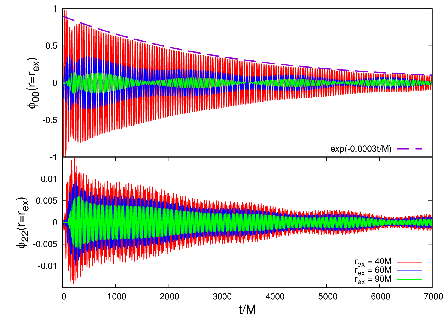

The second noteworthy aspect is that the state keeps, roughly, the symmetry of the initial conditions. This is clearly seen in the energy density plots in Fig. 3. However, it is clear also that fine structure arises, clearly seen for larger binary separations, excited by the presence of the binary, an asymmetric perturber. In particular, we observe the excitation of the quadrupole mode by the BHB. This is clearly shown in Fig. 4, where we show the monopole and quadrupole components of the field at selected “extraction” .
Figure 4 shows that this is indeed a quasibound state, decaying exponentially in time, albeit on long timescales. This is exactly as expected from an analysis of massive fields around nonspinning BHs Brito et al. (2015a). The scalar at late times behaves as an exponentially damped sinusoid, as expected for quasibound states. A fit to the late-time behavior (see Fig. 4) shows that the lifetime of such structures is for , and for . These scales should be compared with the analytical prediction, Eq. (4.13) in Ref. Wong (2020). That expression is applicable to and yields a timescale , in excellent agreement with our numerical results.
| Run | |||
|---|---|---|---|
| nonspin3 | 0.1976 | 0.1973 | |
| spin2 | 0.1992 | 0.1994 | |
| 0.1948 | 0.1951 | ||
| nonspin3 | 0.2012 | 0.2016 | |
| 0.1930 | 0.1930 |
In accordance with our analysis in Sec. II, the scalar field is oscillating with a frequency . To quantify the agreement with the nonrelativistic analysis, we computed the Fourier spectrum of the monopole and quadrupole modes at different radii, and averaged the result. We find clear peaks at different frequencies, the dominant ones are shown in Table 4 for and compared against the nonrelativistic prediction of Sec. II.333One needs to pay attention when comparing against the results of Sec. II, since a rotation of axes is involved and, as we mentioned, at finite separations a spherical harmonic mode maps into a superposition of the states used in Table 1. The agreement is of order 0.1% or better, providing strong evidence that bound, molecular-like gravitational states do form around BHBs. Notice also that we find two (or more) peaks for modes. For we can read from the table that their separation in frequency is , in good agreement with the expected prediction of Sec. III.3, ( for this example).


The interpretation of these states as molecular-like is further supported by the spatial profile of the scalar and energy density, shown in Fig. 5. The time evolution of the energy density along the axis is depicted in the three panels of this figure. The late-time profile around the binary is well described by a density . This profile is in accord with the nonrelativistic, single BH expression [Eq. (16)] for the quasibound state. Our results indicate that this is also a good expression, even for the moderately large separations that we studied. Figure 5 shows that the exponential falloff gives rise to a slowly decaying but small tail of energy density for distances . This looks to be a slow, radiative component part of the signal.
In fact, this gravitational system behaves like a rotating molecule in quantum mechanics.444Disclaimer: one should not read too much in this analogy. The shared electron cloud in a molecule is what binds the atoms together. Here, the “atoms” (two BHs) are bound together by gravity and then the “electron cloud” is a solution of the scalar wave equation on that background. The snapshots of the scalar field and energy density shown in Fig. 3 show that the scalar field is not only localized around the BHB, but that it is dragged by it, rotating counterclockwise, along the orbital motion of the binary. The field shows modulations at low-frequencies—in particular, at —as can be seen in the figures. Such modulation is the expected for an equal-mass binary. Notice that the signal is almost equally modulated in amplitude at different extraction radii; thus the low-frequency envelope is not the result of beatings caused by overtone excitation. In other words the scalar is indeed gravitationally dragged by the binary. The period of such a pattern is the same as the orbital period of the binary.
IV.3 Corotating dipolar global states


The previous evolutions referred to spherically symmetric, momentarily static initial data. We now consider time-asymmetric initial data. Let us focus on dipolar initial data corotating with the binary—i.e., configurations spin1 and spin2 of Table 3. The evolution of the spatial profile of the field and its energy density is shown in Figs. 6 and 7. A dipolar pattern stands out from these plots.
Figures 6 and 7 show that for compact binaries (when the BH separation is smaller than the typical size of the cloud), the energy density of the state acquires a torus-like shape, centered on the binary, and supported by its angular momentum. This is similar to the topology of quasibound states around single BHs. On the other hand, for large BH separations as in Fig. 7, the profile is no longer connected; the torus “breaks up”, and leaves two overdensity clumps of scalar field corotating with the BHB.

The presence of the binary excites other modes with similar symmetries to that in the initial data. In particular, we see a strong octupole mode, shown in Fig. 8 for . Notice that the octupolar mode grows from a negligible value to roughly 10% in amplitude of the dipolar component. Notice also the large timescales involved: the amplitude of these components is approximately constant up to timescales of order or larger. The modulation in the signal is, as we explained before, due to the motion of the binary, and has a frequency as expected for an equal-mass binary.
These results indicate that the evolution drove the system to a quasibound state, a relativistic analogue of the molecular solutions discussed in Sec. II.1 for the nonrelativistic system. Together with the previous results, and as we will insist below, these features indicate that the formation of quasibound states is a robust result for general initial conditions. The analysis of the Fourier-decomposed signal shows a frequency content which is peaked at . This is in good agreement with the nonrelativistic predictions of Sec. II.1 (which yield and , respectively). One finds (see Table 4) , also in very good agreement with the expectations.

The energy density of the configuration is shown in Fig. 9. These results show clearly that the initial conditions are similar to those of a quasibound state, and the system evolution does not take it away significantly from the initial conditions. The asymptotic behavior of the density profile is well described by . Note that the nonrelativistic prediction [Eq. (16)] for the scalar profile is of the form for the fundamental mode when . This is in perfect agreement with our time-evolution results around a BHB.
IV.4 Counterrotating dipolar global states


Similar results hold for the evolution of counterrotating initial data (with respect to the binary, thus data rotating clockwise). We have evolved configuration spin3 of Table 3 and the corresponding profiles of the field and energy density are shown in Fig. 10.
Since the initial profile has angular momentum which is opposite to that of the binary, the scalar field rotates in a direction opposite to the BHB. However, the energy density of the scalar cloud does rotate in the same direction as that of the binary. The asymptotic late-time spatial distribution of the energy density is well described by a radial dependence , consistent with a nonrelativistic analysis of quasibound states.

IV.5 General initial data
We investigated other types of initial conditions, such as narrower pulses, with smaller width . This changes the amount of field that is dissipated in the early stages, but a quasibound state always ends up forming, with a phenomenology similar to what we described.
We also studied data with higher initial frequency content: since quasibound states have , it is conceivable that high-frequency initial data just dissipates away. Our results show that this does not happen. Instead, again, the system evolves towards a frequency content and a spatial distribution described well by a nonrelativistic quasibound state. It seems that these quasibound states are an attractor in the phase space.
We should also add that quasibound states decay exponentially in space, far away from the binary. At large distances, the dominant behavior is controlled by power-law tails Hod and Piran (1998); Koyama and Tomimatsu (2001, 2002); Witek et al. (2013). Asymptotically, our results are consistent with a late-time decay where the exponent at intermediate times, and at very late times. Our results are consistent with analytical predictions Hod and Piran (1998); Koyama and Tomimatsu (2001, 2002); Witek et al. (2013).
Finally, we note that if the quasibound states described above did not exist, the evolution of initial data would lead, on relatively short timescales, to the total depletion of scalar field everywhere. It would quickly be absorbed by the BHs or dispersed to infinity.
V Conclusions
Light scalar fields are interesting solutions to some of the most pressing problems in physics. One example is the dark matter problem. It is tempting to introduce fields with a scale (the Compton wavelength) similar to the size of galactic cores. One would thus be dealing with fields of mass or similar, in what are known as fuzzy dark matter models Robles and Matos (2012); Hui et al. (2017). Understanding the physics and evolution of compact binaries in such environments is crucial to modeling their evolution and to searching for such fields Annulli et al. (2020a, b).
Our results indicate that, in the presence of a background scalar, the scalar field dynamics close to a BHB parallels very closely that of an electron in a one-electron heteronuclear diatomic molecule. We do note that there are very important differences between realistic BHBs and molecules. In particular, a BHB is a dissipative system. Our numerical results for the time evolution of initial data show that nonrelativistic bound states turn into quasibound states, via absorption at the horizon.
A BHB is dissipative in another way, not included (for simplicity) in our simulations: the system loses energy through gravitational wave emission. We focused on timescales much shorter than the typical scale for BH coalescence. Naturally there are systems for which this assumption is not justified. The typical timescale until coalescence is Peters (1964) (for simplicity, we assume a circular orbit and an equal mass binary). The timescale is for , and for . Our numerical simulations clearly show that the quasibound state lifetime is at least . Thus, BHB evolution via gravitational-wave emission is indeed relevant for the evolution of these states, especially at small separations, and left for future work.
We have not dealt with eccentricity, nor did we consider unequal-mass binaries, although it is straightforward to apply our formalism and methods to these situations. Unequal-mass binary evolution might lead, due asymmetric accretion and drag, to substantial center-of-mass velocities making it especially interesting to study Cardoso and Macedo (2020).
In the context of gravitational-wave imprints, dynamical friction caused by such fields and its impact on the gravitational-wave phase was recently described Annulli et al. (2020a, b). However, such description does not include possible quasibound-state formation. The clouds have a size and according to general considerations and specific calculations Feynman (1939) they should contribute an extra attracting force which scales linearly with the scalar density. Since this is a conservative effect, its only consequence is a slight renormalization of the binary mass, and we do not expect changes to the dephasing introduced by dissipative effects Annulli et al. (2020a, b) (in particular, a dephasing appearing at post-Newtonian order “” with respect to the leading vacuum general relativity prediction).
Still in the context of ultralight dark matter, consider a BHB evolving within a “cloud” of coherently oscillating scalars. This cloud could have primordial origin—and be a component of ultralight dark matter, or could simply arise as a consequence of superradiant instabilities, and be localized around a supermassive, spinning BH. Now, when this cloud is much larger than any scale in a BHB system, the corresponding boundary conditions are different. It is possible that molecular-like states arise, but their study requires understanding the time evolution of scalar fields with coherent oscillating boundary conditions Clough et al. (2019).
The tidal disruption of scalar clouds by orbiting companions was recently discussed Cardoso et al. (2020). Our results raise the interesting possibility that the final state of such a disruption can be a gravitational molecule.
We note that the response of BHBs to external fluctuations has been studied recently. In particular, the response to high-frequency and low-frequency scalars was studied in toy models Assumpcao et al. (2018); Nakashi and Igata (2019a, b). A realistic BHB configuration revealed already universal ringdown for binaries, and hints of superradiance Bernard et al. (2019); Wong (2019); Brito et al. (2015a). Together with the results we discussed here, these studies show that compact binaries are a fertile ground for new phenomenology.
Our results can also be put into the context of stationary solutions of the field equations. One can show that minimally coupling gravity to a real scalar field cannot give rise to stationary BH geometries with a nontrivial scalar field—as this would give rise to a time-dependent stress-energy tensor, and hence the emission of gravitational waves—or absorption of the scalar field at the BH horizon. However, these results can be circumvented for single-BH spacetimes if the field is complex (hence giving rise to a time-independent stress-energy tensor) and the BH is spinning (where superradiance prevents absorption by the horizon) Herdeiro and Radu (2014); Brito et al. (2015a). Thus, stationary BH solutions surrounded by scalar fields are possible Herdeiro and Radu (2014). Given the very nature of BH binaries, and the fact that they are bound by gravity and hence evolve via gravitational-wave emission, the existence of stationary solutions is a priori not expected. What we have shown, is that on timescales short compared to those caused by energy loss through gravitational radiation, quasibound states of scalar fields are possible and form naturally.
Acknowledgements.
V.C. acknowledges financial support provided under the European Union’s H2020 ERC Consolidator Grant “Matter and strong-field gravity: New frontiers in Einstein’s theory” grant agreement no. MaGRaTh–646597. M.Z. acknowledges financial support provided by FCT/Portugal through the IF programme, grant IF/00729/2015. T.I. acknowledges financial support provided under the European Union’s H2020 ERC, Starting Grant agreement no. DarkGRA–757480. This project has received funding from the European Union’s Horizon 2020 research and innovation programme under the Marie Sklodowska-Curie grant agreement No 690904. We acknowledge financial support provided by FCT/Portugal through grant PTDC/MAT-APL/30043/2017 and through the bilateral agreement FCT-PHC (Pessoa programme) 2020-2021. The authors would like to acknowledge networking support by the GWverse COST Action CA16104, “Black holes, gravitational waves and fundamental physics.” Computations were performed on the “Baltasar Sete-Sois” cluster at IST and XC40 at YITP in Kyoto University. This work was granted access to the HPC resources of MesoPSL financed by the Region Ile de France and the project Equip@Meso (reference ANR-10-EQPX-29-01) of the programme Investissements d’Avenir supervised by the Agence Nationale pour la Recherche.Appendix A Mode excitation by a binary spacetime
To understand which modes are excited by the BHB let us again consider the metric in Eq. (2). Expanding the Newtonian potential [Eq. (3)], we obtain
| (38) |
The Klein-Gordon equation on this spacetime can be written as
The formal solution of this equation is
where is the homogeneous solution, fixed by the initial data. is the Green’s function,
| (39) |
where , and is a complex conjugate. For weak couplings, ,
| (40) | |||
Let us now expand the right-hand side of this equation in spherical harmonics,
| (41) | ||||
| (42) |
where
and , , , . The Green function can also be expanded in spherical harmonics through the plane wave expansion
where the are the spherical Bessel functions and the hat denotes a unit vector. Thus,
where
Let us consider the modes of the scattered field, . Performing the integration in the angular directions of we obtain
| (43) |
where
This integral is nonzero only when . Since, from Eq. (42), is nonzero only for we see that is nontrivial only when , or , for nontrivial values of .
Appendix B Convergence test
As mentioned in Sec. III.1, for our numerical implementation we approximate spatial derivatives with fourth-order-accurate finite difference stencils and integrate in time with a fourth-order Runge-Kutta scheme. Communication between refinement levels is done by Carpet with second- and fifth-order accuracy in time and space, respectively.
To assess the convergence properties of our results we performed three simulations for configuration nonspin2, with resolutions (on the coarsest refinement level) , , and . We define the usual convergence factor
| (44) |
where is the expected convergence order, and depict the corresponding results for the , multipole of the evolved function in Fig. 12. The results are compatible with a convergence order between orders 2 and 3, which is consistent with the numerical scheme used.

References
- Bekenstein (1972) J. D. Bekenstein, Phys. Rev. D 5, 1239 (1972).
- Robinson (1975) D. Robinson, Phys. Rev. Lett. 34, 905 (1975).
- Bekenstein (1997) J. D. Bekenstein, in Proceedings of the Second International A.D. Sakharov Conference on Physics: Moscow, Russia 20-24 May 1996, edited by I. M. Dremin and A. M. Semikhatov (World Scientific, 1997) arXiv:gr-qc/9605059 [gr-qc] .
- Chrusciel et al. (2012) P. T. Chrusciel, J. L. Costa, and M. Heusler, Living Rev. Relativ. 15, 7 (2012), arXiv:1205.6112 [gr-qc] .
- Brito et al. (2015a) R. Brito, V. Cardoso, and P. Pani, Lect. Notes Phys. 906, pp.1 (2015a), arXiv:1501.06570 [gr-qc] .
- Detweiler (1980) S. L. Detweiler, Phys. Rev. D 22, 2323 (1980).
- Arvanitaki and Dubovsky (2011) A. Arvanitaki and S. Dubovsky, Phys. Rev. D 83, 044026 (2011), arXiv:1004.3558 [hep-th] .
- Baumann et al. (2019a) D. Baumann, H. S. Chia, J. Stout, and L. ter Haar, JCAP 12, 006 (2019a), arXiv:1908.10370 [gr-qc] .
- Sanchis-Gual et al. (2020) N. Sanchis-Gual, M. Zilhão, C. Herdeiro, F. Di Giovanni, J. A. Font, and E. Radu, (2020), arXiv:2007.11584 [gr-qc] .
- Clough et al. (2018) K. Clough, T. Dietrich, and J. C. Niemeyer, Phys. Rev. D 98, 083020 (2018), arXiv:1808.04668 [gr-qc] .
- Brito et al. (2015b) R. Brito, V. Cardoso, and P. Pani, Class. Quant. Grav. 32, 134001 (2015b), arXiv:1411.0686 [gr-qc] .
- Yoshino and Kodama (2014) H. Yoshino and H. Kodama, PTEP 2014, 043E02 (2014), arXiv:1312.2326 [gr-qc] .
- Herdeiro and Radu (2014) C. A. R. Herdeiro and E. Radu, Phys. Rev. Lett. 112, 221101 (2014), arXiv:1403.2757 [gr-qc] .
- Bernard et al. (2019) L. Bernard, V. Cardoso, T. Ikeda, and M. Zilhão, Phys. Rev. D 100, 044002 (2019), arXiv:1905.05204 [gr-qc] .
- Wong (2020) L. K. Wong, Phys. Rev. D 101, 124049 (2020), arXiv:2004.03570 [hep-th] .
- Baumann et al. (2019b) D. Baumann, H. S. Chia, and R. A. Porto, Phys. Rev. D 99, 044001 (2019b), arXiv:1804.03208 [gr-qc] .
- Burrau (1927) Ø. Burrau, Danske Vidensk. Selskab. Math.-fys. Meddel. (in German) M 7, 1 (1927).
- Wilson (1928) A. H. Wilson, Proceedings of the Royal Society of London A118, 635 (1928).
- Brown and Steiner (1966) W. B. Brown and E. Steiner, The Journal of Chemical Physics 44, 3934 (1966), https://doi.org/10.1063/1.1726555 .
- Nickel (2011) B. Nickel, Journal of Physics A: Mathematical and Theoretical 44, 395301 (2011).
- Leaver (1986) E. W. Leaver, Journal of Mathematical Physics 27, 1238 (1986).
- Berti et al. (2006) E. Berti, V. Cardoso, and M. Casals, Phys. Rev. D73, 024013 (2006), [Erratum: Phys. Rev.D73,109902(2006)], arXiv:gr-qc/0511111 [gr-qc] .
- Bates and Reid (1968) D. Bates and R. Reid, Electronic Eigenenergies of the Hydrogen Molecular Ion, edited by D. Bates and I. Estermann, Advances in Atomic and Molecular Physics, Vol. 4 (Academic Press, 1968) pp. 13 – 35.
- Bethe (1933) H. Bethe, Handbuch der Physik, edited by S. Flugge, Vol. 24 (Springer, 1933) p. 527.
- Abramov and Slavyanov (2001) D. Abramov and S. Slavyanov, Journal of Physics B: Atomic and Molecular Physics 11, 2229 (2001).
- Damburg et al. (1984) R. J. Damburg, R. K. Propin, S. Graffi, V. Grecchi, E. M. Harrell, J. c. v. Čížek, J. Paldus, and H. J. Silverstone, Phys. Rev. Lett. 52, 1112 (1984).
- Cardoso et al. (2009) V. Cardoso, A. S. Miranda, E. Berti, H. Witek, and V. T. Zanchin, Phys. Rev. D79, 064016 (2009), arXiv:0812.1806 [hep-th] .
- Weinberg (2015) S. Weinberg, Lectures on Quantum Mechanics, 2nd ed. (Cambridge University Press, 2015).
- Mundim et al. (2014) B. C. Mundim, H. Nakano, N. Yunes, M. Campanelli, S. C. Noble, and Y. Zlochower, Phys. Rev. D89, 084008 (2014), arXiv:1312.6731 [gr-qc] .
- Johnson-McDaniel et al. (2009) N. K. Johnson-McDaniel, N. Yunes, W. Tichy, and B. J. Owen, Physical Review D 80 (2009), 10.1103/physrevd.80.124039.
- Löffler et al. (2012) F. Löffler, J. Faber, E. Bentivegna, T. Bode, P. Diener, R. Haas, I. Hinder, B. C. Mundim, C. D. Ott, E. Schnetter, G. Allen, M. Campanelli, and P. Laguna, Class. Quantum Grav. 29, 115001 (2012), arXiv:1111.3344 [gr-qc] .
- Zilhão and Löffler (2013) M. Zilhão and F. Löffler, Proceedings, Spring School on Numerical Relativity and High Energy Physics (NR/HEP2): Lisbon, Portugal, March 11-14, 2013, Int. J. Mod. Phys. A28, 1340014 (2013), arXiv:1305.5299 [gr-qc] .
- Babiuc-Hamilton et al. (2019) M. Babiuc-Hamilton et al., (2019), 10.5281/zenodo.3522086, http://einsteintoolkit.org.
- Schnetter et al. (2004) E. Schnetter, S. H. Hawley, and I. Hawke, Class. Quant. Grav. 21, 1465 (2004), arXiv:gr-qc/0310042 [gr-qc] .
- (35) Carpet, Carpet: Adaptive Mesh Refinement for the Cactus Framework.
- Pollney et al. (2011) D. Pollney, C. Reisswig, E. Schnetter, N. Dorband, and P. Diener, Physical Review D 83 (2011), 10.1103/physrevd.83.044045.
- Witek et al. (2020) H. Witek, M. Zilhao, G. Ficarra, and M. Elley, (2020), 10.5281/zenodo.3565475.
- Cunha et al. (2017) P. V. P. Cunha, J. A. Font, C. Herdeiro, E. Radu, N. Sanchis-Gual, and M. Zilhão, Phys. Rev. D96, 104040 (2017), arXiv:1709.06118 [gr-qc] .
- Assumpcao et al. (2018) T. Assumpcao, V. Cardoso, A. Ishibashi, M. Richartz, and M. Zilhao, Phys. Rev. D98, 064036 (2018), arXiv:1806.07909 [gr-qc] .
- Hod and Piran (1998) S. Hod and T. Piran, Phys. Rev. D 58, 044018 (1998), arXiv:gr-qc/9801059 .
- Koyama and Tomimatsu (2001) H. Koyama and A. Tomimatsu, Phys. Rev. D 64, 044014 (2001), arXiv:gr-qc/0103086 .
- Koyama and Tomimatsu (2002) H. Koyama and A. Tomimatsu, Phys. Rev. D 65, 084031 (2002), arXiv:gr-qc/0112075 .
- Witek et al. (2013) H. Witek, V. Cardoso, A. Ishibashi, and U. Sperhake, Phys. Rev. D87, 043513 (2013), arXiv:1212.0551 [gr-qc] .
- Robles and Matos (2012) V. H. Robles and T. Matos, Mon. Not. Roy. Astron. Soc. 422, 282 (2012), arXiv:1201.3032 [astro-ph.CO] .
- Hui et al. (2017) L. Hui, J. P. Ostriker, S. Tremaine, and E. Witten, Phys. Rev. D95, 043541 (2017), arXiv:1610.08297 [astro-ph.CO] .
- Annulli et al. (2020a) L. Annulli, V. Cardoso, and R. Vicente, Phys. Lett. B 811, 135944 (2020a), arXiv:2007.03700 [astro-ph.HE] .
- Annulli et al. (2020b) L. Annulli, V. Cardoso, and R. Vicente, Phys. Rev. D 102, 063022 (2020b), arXiv:2009.00012 [gr-qc] .
- Peters (1964) P. Peters, Phys. Rev. 136, B1224 (1964).
- Cardoso and Macedo (2020) V. Cardoso and C. F. Macedo, Mon. Not. Roy. Astron. Soc. 498, 1963 (2020), arXiv:2008.01091 [astro-ph.HE] .
- Feynman (1939) R. Feynman, Phys. Rev. 56, 340 (1939).
- Clough et al. (2019) K. Clough, P. G. Ferreira, and M. Lagos, Phys. Rev. D 100, 063014 (2019), arXiv:1904.12783 [gr-qc] .
- Cardoso et al. (2020) V. Cardoso, F. Duque, and T. Ikeda, Phys. Rev. D 101, 064054 (2020), arXiv:2001.01729 [gr-qc] .
- Nakashi and Igata (2019a) K. Nakashi and T. Igata, Phys. Rev. D 99, 124033 (2019a), arXiv:1903.10121 [gr-qc] .
- Nakashi and Igata (2019b) K. Nakashi and T. Igata, Phys. Rev. D 100, 104006 (2019b), arXiv:1908.10075 [gr-qc] .
- Wong (2019) L. K. Wong, Phys. Rev. D 100, 044051 (2019), arXiv:1905.08543 [hep-th] .