Björling problem for zero mean curvature surfaces in the three-dimensional light cone

Joseph Cho Institute of Discrete Mathematics and Geometry, TU Wien, Wien, 1040, Austria [email protected] , So Young Kim Department of Mathematics, Korea University, Seoul, 02841, Republic of Korea [email protected] , Dami Lee Department of Mathematics, Indiana University, Bloomington, IN, 47405, USA [email protected] , Wonjoo Lee Department of Mathematics, Korea University, Seoul, 02841, Republic of Korea [email protected] and Seong-Deog Yang Department of Mathematics, Korea University, Seoul, 02841, Republic of Korea [email protected]

Abstract.

We solve the Björling problem for zero mean curvature surfaces in the three-dimensional light cone. As an application, we construct and classify all rotational zero mean curvature surfaces.

Key words and phrases:

Zero mean curvature surfaces, Björling representation

2020 Mathematics Subject Classification:

Primary 53A10; Secondary 53B30.

1. Introduction

The classical Björling problem [bjorling_integrationem_1844] poses the following question: Suppose that a curve $\gamma\mathrel{\mathop{\ordinarycolon}}I\to\mathbb{E}^{3}$ and a unit vector field $N$ along $\gamma$ in the Euclidean 3-space $\mathbb{E}^{3}$ are given so that

\dot{\gamma}\cdot N=0,

where $\dot{\phantom{\gamma}}$ denotes the differentiation with respect to $u\in I$ , and $\cdot$ is the standard Euclidean inner product. The goal is to find a minimal surface $X$ which contains $\gamma$ and whose unit normal along $\gamma$ is the prescribed $N$ . Due to the Weierstrass representation of minimal surfaces [weierstrass_untersuchungen_1866], this problem can be solved via analytic extensions of $\gamma$ and $N$ to the complex plane:

X(z)=\int_{u_{0}}^{z}(\dot{\gamma}(w)-iN(w)\times\dot{\gamma}(w))\operatorname{d\!}{w}

where $\times$ denotes the standard Euclidean cross product. The curve and the prescribed normal together are called the Björling data. Such Björling type problems are well studied across various types of surfaces in various space forms (see, for example, [alias_bjorling_2003, asperti_bjorling_2006, brander_bjorling_2010, brander_bjorling_2018, dussan_bjorling_2017, kim_spacelike_2011, kim_prescribing_2007, yang_bjorling_2017]).

The Björling data can be slightly modified by noting that $\mathcal{L}\mathrel{\mathop{\ordinarycolon}}=N\times\dot{\gamma}$ is perpendicular to $\dot{\gamma}$ and of the same length to $\dot{\gamma}$ . Thus if $\mathcal{L}$ is prescribed then one can recover $N$ via $N=\frac{\dot{\gamma}\times\mathcal{L}}{|\dot{\gamma}\times\mathcal{L}|}$ , allowing us to adopt $\gamma$ and $\mathcal{L}$ instead of $\gamma$ and $N$ as Björling data. Geometrically, the vector field $\mathcal{L}$ of the Björling data is equivalent to the prescription of the tangent vector field of the surface that is perpendicular to $\dot{\gamma}$ along $\gamma$ . This change in viewpoint of the prescribed data for the Björling problem proved to be useful for obtaining the (singular) Björling representation [kim_prescribing_2007] for maxfaces [umehara_maximal_2006] and generalized timelike minimal surfaces [kim_spacelike_2011] in Lorentz $3$ -space, and also the Björling representation for zero mean curvature surfaces in isotropic $3$ -space [seo_zero_2021].

Our goal of the paper is to solve the Björling problem for zero mean curvature surfaces in the $3$ -dimensional light cone $\mathbb{Q}^{3}_{+}$ . In the similar cases of other quadrics of Lorentz $4$ -space, namely, the hyperbolic $3$ -space $\mathbb{H}^{3}(-1)$ and de Sitter $3$ -space $\mathbb{S}^{3}_{1}(1)$ , the tangent space is isomorphic to either the Euclidean $3$ -space or the Lorentz $3$ -space, respectively. Thus one can use the cross product in the tangent space to obtain Björling representations [yang_bjorling_2017] in an analogous manner to the Euclidean case. However, the tangent space to $\mathbb{Q}^{3}_{+}$ is isomorphic to isotropic $3$ -space, so that it does not have a cross product structure. Therefore, for the Björling problem in $\mathbb{Q}^{3}_{+}$ , we use the alternative viewpoint and assume that the given Björling data consists of a spacelike analytic curve $\gamma$ , together with a spacelike vector field $\mathcal{L}$ along the curve, and find the zero mean curvature surface which contains $\gamma$ and has $\mathcal{L}$ as a tangent vector field along $\gamma$ .

The paper is structured as follows: After reviewing the basic geometry and surface theory of $\mathbb{Q}^{3}_{+}$ in Section 2, we describe the process to solve the Björling problem for a given spacelike analytic curve with prescribed tangent vector field in Section 3, culminating in the Björling representation for zero mean curvature surfaces in $3$ -dimensional light cone (see Theorem 3.8). As an application, we construct and classify (see Theorem 4.4) rotationally invariant zero mean curvature surfaces in $\mathbb{Q}^{3}_{+}$ in Section 4. Furthermore, many surfaces admitting Weierstrass representations in various space forms with indefinite metric can be extended across lightlike lines (see, for example, [akamine_reflection_2021, akamine_reflection_2022, akamine_space-like_2019, fujimori_analytic_2022, fujimori_zero_2015-1, umehara_hypersurfaces_2019]); we give an example of such surface in $\mathbb{Q}^{3}_{+}$ in Section 4.5.

2. Preliminaries

We first briefly review the geometry of three-dimensional light cone, and the surface theory within. For a detailed description, see [liu_surfaces_2007, liu_hypersurfaces_2008, liu_representation_2011].

2.1. Hermitian matrix model of three-dimensional light cone

Let $\mathbb{L}^{4}$ denote the Lorentz $4$ -space, with inner product

\langle(t_{1},x_{1},y_{1},z_{1}),(t_{2},x_{2},y_{2},z_{2})\rangle=-t_{1}t_{2}+x_{1}x_{2}+y_{1}y_{2}+z_{1}z_{2}.

The Lorentz $4$ -space can be identified with the set of $2\times 2$ Hermitian matrices $\mathrm{Herm}(2,\mathbb{C})$ via

(t,x,y,z)\sim\begin{pmatrix}t+z&x+iy\\ x-iy&t-z\end{pmatrix}

where we will abuse notation between vectors and matrices. Then for any $V,W\in\mathrm{Herm}(2,\mathbb{C})\cong\mathbb{L}^{4}$ ,

\langle V,W\rangle=-\frac{1}{2}\left(\det{(V+W)}-\det{V}-\det{W}\right),

so that

|V|^{2}\mathrel{\mathop{\ordinarycolon}}=\langle V,V\rangle=-\det{V}.

We note here that the symmetric bilinear form $\langle\cdot,\cdot\rangle$ is well-defined for all $A\in\mathrm{M}(2,\mathbb{C})$ .

Defining

f_{0}\mathrel{\mathop{\ordinarycolon}}=\begin{pmatrix}0&0\\ 0&-2\end{pmatrix},\quad f_{1}\mathrel{\mathop{\ordinarycolon}}=\begin{pmatrix}0&1\\ 1&0\end{pmatrix},\quad f_{2}\mathrel{\mathop{\ordinarycolon}}=\begin{pmatrix}0&i\\ -i&0\end{pmatrix},\quad f_{3}\mathrel{\mathop{\ordinarycolon}}=\begin{pmatrix}1&0\\ 0&0\end{pmatrix},

we see that $\{f_{0},f_{1},f_{2},f_{3}\}$ form an asymptotically orthonormal basis of $\mathbb{L}^{4}\cong\mathrm{Herm}(2,\mathbb{C})$ .

In the Hermitian model, hyperbolic $3$ -space $\mathbb{H}^{3}(-1)$ , $3$ -dimensional light cone $\mathbb{Q}^{3}_{+}$ , and de Sitter $3$ -space $\mathbb{S}^{3}_{1}(1)$ can be defined as quadrics in $\mathbb{L}^{4}$ via

	$\displaystyle\mathbb{H}^{3}(-1)$	$\displaystyle\mathrel{\mathop{\ordinarycolon}}=\{X\in\mathrm{Herm}(2,\mathbb{C})\mathrel{\mathop{\ordinarycolon}}\langle X,X\rangle=-1,\operatorname{tr}{X}>0\},$
	$\displaystyle\mathbb{Q}^{3}_{+}$	$\displaystyle\mathrel{\mathop{\ordinarycolon}}=\{X\in\mathrm{Herm}(2,\mathbb{C})\mathrel{\mathop{\ordinarycolon}}\langle X,X\rangle=0,\operatorname{tr}{X}>0\},$
	$\displaystyle\mathbb{S}^{3}_{1}(1)$	$\displaystyle\mathrel{\mathop{\ordinarycolon}}=\{X\in\mathrm{Herm}(2,\mathbb{C})\mathrel{\mathop{\ordinarycolon}}\langle X,X\rangle=1\},$

respectively. Note that for any $X\in\mathbb{Q}^{3}_{+}$ , there is some $F\in\mathrm{SL}(2,\mathbb{C})$ such that

X=F\begin{pmatrix}1&0\\ 0&0\end{pmatrix}F^{\star}=Ff_{3}F^{\star}

where $F^{\star}$ denotes the conjugate transpose of $F$ .

When we visualize surfaces in $\mathbb{Q}^{3}_{+}$ , we will use the following stereographic projection

\mathbb{Q}^{3}_{+}\ni(t,x,y,z)\mapsto\left(\frac{x}{1+t},\frac{y}{1+t},\frac{z}{1+t}\right).

Then $\mathbb{Q}^{3}_{+}$ is identified with $\{(a,b,c)\in\mathbb{R}^{3}\mathrel{\mathop{\ordinarycolon}}0<a^{2}+b^{2}+c^{2}<1\}$ .

2.2. Surface theory and Weierstrass-type representation

Let $D$ be a two-dimensional simply-connected domain, and suppose $X\mathrel{\mathop{\ordinarycolon}}D\to\mathbb{Q}^{3}_{+}$ is a spacelike immersion, that is, the induced metric on the tangent plane of $X$ at every point $p\in D$ is Riemannian. Then for conformal coordinates $(u,v)\in D$ with complex structure given via $z=u+iv$ , suppose that the first fundamental form is given by

\operatorname{d\!}{s}^{2}=\phi^{2}(\operatorname{d\!}{u}^{2}+\operatorname{d\!}{v}^{2})=\phi^{2}\operatorname{d\!}{z}\operatorname{d\!}{\bar{z}}

for some $\phi\mathrel{\mathop{\ordinarycolon}}D\to\mathbb{R}^{\times}$ . Furthermore, we have $\langle X,X_{u}\rangle=\langle X,X_{v}\rangle=0$ so that there exists a unique lightlike $n\mathrel{\mathop{\ordinarycolon}}D\to\mathbb{L}^{4}$ such that

(2.1)

\langle n,n\rangle=\langle n,X_{u}\rangle=\langle n,X_{v}\rangle=0,\quad\langle n,X\rangle=1.

Such $n$ is called the Gauss map of $X$ , and the coefficients of the second fundamental form is then computed in terms of $n$ via

L\mathrel{\mathop{\ordinarycolon}}=-\langle X_{u},n_{u}\rangle,\quad M\mathrel{\mathop{\ordinarycolon}}=-\langle X_{u},n_{v}\rangle=-\langle X_{v},n_{u}\rangle,\quad N\mathrel{\mathop{\ordinarycolon}}=-\langle X_{v},n_{v}\rangle.

Hence, the shape operator $S$ is

S=\phi^{-2}\begin{pmatrix}L&M\\ M&N\end{pmatrix}

with the (extrinsic) Gaussian curvature $K$ and mean curvature $H$ given by

K=\det{S},\quad H=\frac{1}{2}\operatorname{tr}S.

Those surfaces $X$ with $H\equiv 0$ will be referred to as zero mean curvature surfaces.

We recall the Weierstrass-type representation for zero mean curvature surfaces in the three-dimensional light cone [liu_representation_2011, Theorem 3.2] (see also [pember_weierstrass-type_2020, § 4.2] and [seo_zero_2021, Theorem 39]):

Fact 2.1.

Any zero mean curvature surface $X\mathrel{\mathop{\ordinarycolon}}D\to\mathbb{Q}^{3}_{+}$ can locally be represented as

X=Ff_{3}F^{\star}=F\begin{pmatrix}1&0\\ 0&0\end{pmatrix}F^{\star}

where $F\mathrel{\mathop{\ordinarycolon}}D\to\mathrm{SL}(2,\mathbb{C})$ satisfies

\operatorname{d\!}{F}F^{-1}=\begin{pmatrix}G&-G^{2}\\ 1&-G\end{pmatrix}\Omega

for some meromorphic function $G\mathrel{\mathop{\ordinarycolon}}D\to\mathbb{C}$ and holomorphic $1$ -form $\Omega\mathrel{\mathop{\ordinarycolon}}D\to\mathbb{C}$ such that $G^{2}\Omega$ is holomorphic. The pair $(G,\Omega)$ is called the Weierstrass data.

3. Solution of the Björling problem

Using the Weierstrass-type representation in Fact 2.1, we will now solve the Björling problem for zero mean curvature surfaces in $\mathbb{Q}^{3}_{+}$ . Unlike the cases of hyperbolic $3$ -space $\mathbb{H}^{3}(-1)$ and de Sitter $3$ -space $\mathbb{S}^{3}_{1}(1)$ , the Björling data we consider will be an analytic curve together with a tangent vector field due to the lack of cross product structure in the tangent space of $\mathbb{Q}^{3}_{+}$ .

3.1. The conformality condition for the Björling data

For an interval $I$ with parameter $u\in I$ , let $\gamma\mathrel{\mathop{\ordinarycolon}}I\to\mathbb{Q}^{3}_{+}$ be a spacelike analytic curve and $\mathcal{L}$ be an analytic spacelike vector field along $\gamma$ such that

(3.1)

\langle\dot{\gamma},\dot{\gamma}\rangle=\langle\mathcal{L},\mathcal{L}\rangle,\quad\langle\dot{\gamma},\mathcal{L}\rangle=0,\quad\langle\gamma,\mathcal{L}\rangle=0.

Geometrically, the conditions (3.1) ensure that $\mathcal{L}$ will be a tangent vector field; thus, we refer to (3.1) as the conformality condition. Our goal is to find a zero mean curvature surface $X\mathrel{\mathop{\ordinarycolon}}D\to\mathbb{Q}^{3}_{+}$ which contains $\gamma$ and which has $\mathcal{L}$ as a tangent vector field along $\gamma$ .

Note that if there is a such a zero mean curvature surface $X$ , then

(3.2)

\operatorname{d\!}{X}=\operatorname{d\!}{F}f_{3}F^{\star}=\operatorname{d\!}{F}F^{-1}Ff_{3}F^{\star}=\begin{pmatrix}G&-G^{2}\\ 1&-G\end{pmatrix}\Omega X=\mathrel{\mathop{\ordinarycolon}}\mathbf{\Omega}X.

Thus, from $\gamma$ and $\mathcal{L}$ , we will construct such $1$ -form $\mathbf{\Omega}$ .

Remark 3.1.

An important distinction from the cases of $\mathbb{H}^{3}(-1)$ and $\mathbb{S}^{3}_{1}(1)$ is that $X\in\mathbb{Q}^{3}_{+}$ is not invertible since $\det X=0$ . Thus, instead of considering $\operatorname{d\!}{X}X^{-1}$ as in the cases of $\mathbb{H}^{3}(-1)$ and $\mathbb{S}^{3}_{1}(1)$ , we consider the equation as in (3.2).

For Björling data $\gamma$ and $\mathcal{L}$ satisfying conformality condition (3.1), let $\gamma(u)=X(u,0)$ and $\mathcal{L}(u)\mathrel{\mathop{\ordinarycolon}}=X_{v}(u,0)$ . Then on one dimensional domain $I$ , (3.2) implies that we must solve for $\mathbf{\Omega}=\mathrel{\mathop{\ordinarycolon}}\tilde{\Omega}\operatorname{d\!}{u}$ satisfying

(3.3)

\Lambda(u)\mathrel{\mathop{\ordinarycolon}}=\frac{1}{2}(\dot{\gamma}(u)-i\mathcal{L}(u))=X_{z}(u,0)=\tilde{\Omega}(u)X(u,0)=\tilde{\Omega}(u)\gamma(u).

We claim that there is a unique $\tilde{\Omega}$ which solves (3.3).

Note that $\det{\Lambda}=0$ because of (3.1), and that $\det{\gamma}=0$ since it is a curve in $\mathbb{Q}^{3}_{+}$ . By standard theory we know that

\det{\tilde{\Omega}}=\operatorname{tr}{\tilde{\Omega}}=0.

Therefore

\mathbf{\Omega}=\begin{pmatrix}G&-G^{2}\\ 1&-G\end{pmatrix}\Omega

for some functions $G$ and $1$ -form $\Omega$ . We rewrite (3.3) as

(3.4)

\begin{pmatrix}\Lambda_{11}&\Lambda_{12}\\ \Lambda_{21}&\Lambda_{22}\end{pmatrix}=\begin{pmatrix}G\tilde{\Omega}&-G^{2}\tilde{\Omega}\\ \tilde{\Omega}&-G\tilde{\Omega}\end{pmatrix}\begin{pmatrix}\gamma_{11}&\gamma_{12}\\ \gamma_{21}&\gamma_{22}\end{pmatrix}.

By examining $(1,1)$ and $(2,1)$ components of (3.4), we see that $G=G_{1}$ and $\tilde{\Omega}=\tilde{\Omega}_{1}$ where

(3.5)

G_{1}=\frac{\Lambda_{11}}{\Lambda_{21}},\quad\tilde{\Omega}_{1}=\frac{\Lambda_{21}^{2}}{\Lambda_{21}\gamma_{11}-\Lambda_{11}\gamma_{21}}.

On the other hand, by examining $(1,2)$ and $(2,2)$ components of (3.4), we see that $G=G_{2}$ and $\tilde{\Omega}=\tilde{\Omega}_{2}$ where

(3.6)

G_{2}=\frac{\Lambda_{12}}{\Lambda_{22}},\quad\tilde{\Omega}_{2}=\frac{\Lambda_{22}^{2}}{\Lambda_{22}\gamma_{12}-\Lambda_{12}\gamma_{22}}.

It is immediate to see $G_{1}=G_{2}$ from the fact that $\det{\Lambda}=0$ . Then

	$\displaystyle\tilde{\Omega}_{1}$	$\displaystyle=\frac{\Lambda_{21}^{2}}{\Lambda_{21}\gamma_{11}-\frac{\Lambda_{12}\Lambda_{21}}{\Lambda_{22}}\gamma_{21}}=\frac{\Lambda_{21}\Lambda_{22}}{\Lambda_{22}\gamma_{11}-\Lambda_{12}\gamma_{21}},$
	$\displaystyle\tilde{\Omega}_{2}$	$\displaystyle=\frac{\Lambda_{22}^{2}}{\Lambda_{22}\gamma_{12}-\frac{\Lambda_{11}\Lambda_{22}}{\Lambda_{21}}\gamma_{22}}=\frac{\Lambda_{21}\Lambda_{22}}{\Lambda_{21}\gamma_{12}-\Lambda_{11}\gamma_{22}}.$

Hence, it is enough to show that the denominators are the same.

For this matter, we multiply (3.4) with the adjunct of $\gamma$ from the right to obtain

\begin{pmatrix}\Lambda_{11}&\Lambda_{12}\\ \Lambda_{21}&\Lambda_{22}\end{pmatrix}\begin{pmatrix}\gamma_{22}&-\gamma_{12}\\ -\gamma_{21}&\gamma_{11}\end{pmatrix}=\begin{pmatrix}G\tilde{\Omega}&-G^{2}\tilde{\Omega}\\ \tilde{\Omega}&-G\tilde{\Omega}\end{pmatrix}\begin{pmatrix}\det{\gamma}&0\\ 0&\det{\gamma}\end{pmatrix}.

However, we have that $\det{\gamma}=0$ since it is a curve in $\mathbb{Q}^{3}_{+}$ . Therefore, the left hand side is a zero matrix. In particular, its trace is 0; hence

\Lambda_{11}\gamma_{22}-\Lambda_{12}\gamma_{21}-\Lambda_{21}\gamma_{12}+\Lambda_{22}\gamma_{11}=0,

implying that $\tilde{\Omega}_{1}=\tilde{\Omega}_{2}$ .

Now, the expressions for $\tilde{\Omega}_{1}$ and $\tilde{\Omega}_{2}$ in (3.5) and (3.6) implies that the Björling data $\gamma$ and $\mathcal{L}$ satisfying (3.1) must additionally satisfy

(3.7)

\gamma_{11}\Lambda_{21}-\gamma_{21}\Lambda_{11}\neq 0.

Unfortunately, the conformality conditions (3.1) alone does not guarantee this; one can even construct explicit examples where the expression (3.7) vanishes for some Björling data satisfying the conformality conditions.

3.2. The orientability condition for the Björling data

To give a geometric interpretation of the condition (3.7), we define the following notion.

Definition 3.2.

For two linearly independent spacelike vectors $U,V\in\mathbb{L}^{4}$ spanning a Riemannian subspace $W$ of $\mathbb{L}^{4}$ , let $\{e_{1},e_{2}\}$ be an orthonormal basis of $W$ such that there is some $F\in\mathrm{SL}(2,\mathbb{C})$ with $Ff_{i}F^{\star}=e_{i}$ for $i=1,2$ . The signed area of $U$ and $V$ , denoted by $\mathrm{SA}(U,V)$ , is defined via

U\wedge V=\mathrel{\mathop{\ordinarycolon}}\mathrm{SA}(U,V)e_{1}\wedge e_{2}.

An important feature of the signed area is the fact that it is invariant under orientation-preserving isometries of $\mathbb{Q}^{3}_{+}$ . On the other hand, the square of the signed area (or the squared area) can be calculated using the inner product of the ambient Lorentz $4$ -space:

Lemma 3.3.

For linearly independent spacelike vectors $U,V$ spanning a Riemannian subspace $W$ , we have

\mathrm{SA}(U,V)^{2}=\langle U,U\rangle\langle V,V\rangle-\langle U,V\rangle^{2}.

Proof.

Let $\{e_{1},e_{2}\}$ be an orthonormal basis $W$ such that $Ff_{i}F^{\star}=e_{i}$ for $i=1,2$ with $F\in\mathrm{SL}(2,\mathbb{C})$ . Writing

U=ae_{1}+be_{2},\quad V=ce_{1}+de_{2}

for some constants $a,b,c,d\in\mathbb{R}$ , we calculate that

\mathrm{SA}(U,V)e_{1}\wedge e_{2}=(ae_{1}+be_{2})\wedge(ce_{1}+de_{2})=(ad-bc)e_{1}\wedge e_{2}.

On the other hand, we have

\langle U,U\rangle\langle V,V\rangle-\langle U,V\rangle^{2}=(a^{2}+b^{2})(c^{2}+d^{2})-(ac+bd)^{2}=(ad-bc)^{2},

giving us the desired conclusion. ∎

The next lemmata give additional geometric criteria for the Björling data to satisfy (3.7) in terms of the signed area.

Lemma 3.4.

Given Björling data $\gamma$ and $\mathcal{L}$ satisfying the conformality condition, the signed area of $\dot{\gamma}$ and $\mathcal{L}$ does not vanish.

Proof.

Suppose for contradiction that $\mathrm{SA}(\dot{\gamma},\mathcal{L})=0$ . Then direct calculations show that $\mathcal{\mathcal{L}}=\alpha\gamma\pm\dot{\gamma}$ for some $\alpha$ . Thus

\pm\langle\dot{\gamma},\dot{\gamma}\rangle=\langle\dot{\gamma},\alpha\gamma\pm\dot{\gamma}\rangle=\langle\dot{\gamma},\mathcal{L}\rangle=0,

which is a contradiction since $\dot{\gamma}$ is spacelike. ∎

Lemma 3.5.

Given Björling data $\gamma$ and $\mathcal{L}$ satisfying the conformality condition, $G$ and $\Omega$ are well-defined if and only if the signed area of $\dot{\gamma}$ and $\mathcal{L}$ is negative.

Proof.

Fix any $u_{0}\in I$ throughout the proof. Since signed area is invariant under orientation-preserving isometries, we may assume without loss of generality that $\gamma=2f_{3}$ , so that any vector in $T_{\gamma}\mathbb{Q}^{3}_{+}$ takes the form

\ell\gamma+xf_{1}+yf_{2}

for some $\ell,x,y\in\mathbb{R}$ . By the conformality conditions (3.1) on the Björling data, we have that $\dot{\gamma},\mathcal{L}\in T_{\gamma}\mathbb{Q}^{3}_{+}$ ; therefore, there are some constants $a,b,c,d,e,f\in\mathbb{R}$ such that

\dot{\gamma}=a\gamma+bf_{1}+cf_{2},\quad\text{and}\quad\mathcal{L}=d\gamma+ef_{1}+ff_{2}.

Since $\Lambda\mathrel{\mathop{\ordinarycolon}}=\frac{1}{2}\left(\dot{\gamma}-i\mathcal{L}\right)$ , we calculate that

\displaystyle\gamma_{11}\Lambda_{21}-\gamma_{21}\Lambda_{11}=(b-f)-i(c+e),

so that

(3.8)	$\displaystyle\|\gamma_{11}\Lambda_{21}-\gamma_{21}\Lambda_{11}\|^{2}$	$\displaystyle=b^{2}+c^{2}+e^{2}+f^{2}+2(ce-bf)$
		$\displaystyle=\|\dot{\gamma}\|^{2}+\|\mathcal{L}\|^{2}+2(ce-bf)$
		$\displaystyle=2(\|\dot{\gamma}\|^{2}-(bf-ce)).$

Now since $\gamma$ -component does not affect the signed area, we note that

\mathrm{SA}(\dot{\gamma},\mathcal{L})=\mathrm{SA}(bf_{1}+cf_{2},ef_{1}+ff_{2}).

However, we can also calculate that

\mathrm{SA}(bf_{1}+cf_{2},ef_{1}+ff_{2})f_{1}\wedge f_{2}=(bf_{1}+cf_{2})\wedge(ef_{1}+ff_{2})=(bf-ce)f_{1}\wedge f_{2},

allowing us to deduce that

\mathrm{SA}(\dot{\gamma},\mathcal{L})=bf-ce.

On the other hand, Lemma 3.3 and the conformality conditions (3.1) imply that

\mathrm{SA}(\dot{\gamma},\mathcal{L})^{2}=|\dot{\gamma}|^{2}|\mathcal{L}|^{2}-\langle\dot{\gamma},\mathcal{L}\rangle^{2}=|\dot{\gamma}|^{4}

so that

bf-ce=\mathrm{SA}(\dot{\gamma},\mathcal{L})=\begin{cases}|\dot{\gamma}|^{2},&\text{if }\mathrm{SA}(\dot{\gamma},\mathcal{L})>0,\\ -|\dot{\gamma}|^{2},&\text{if }\mathrm{SA}(\dot{\gamma},\mathcal{L})<0.\end{cases}

Thus, using (3.8) allows us to conclude that

|\gamma_{11}\Lambda_{21}-\gamma_{21}\Lambda_{11}|^{2}=\begin{cases}0,&\text{if }\mathrm{SA}(\dot{\gamma},\mathcal{L})>0,\\ 4|\dot{\gamma}|^{2},&\text{if }\mathrm{SA}(\dot{\gamma},\mathcal{L})<0.\end{cases}

Therefore, $G$ and $\Omega$ are well-defined if and only if $SA(\dot{\gamma},\mathcal{L})<0$ . ∎

Remark 3.6.

The signed area condition of Lemma 3.5 encodes the fact that the orientation of $\dot{\gamma}$ and $\mathcal{L}$ must be correct. For this reason, we call the signed area condition, the orientability condition.

Remark 3.7.

The orientability condition is unnecessary for the Björling data in other quadrics such as $\mathbb{H}^{3}(-1)$ and $\mathbb{S}^{3}_{1}(1)$ ; the crucial difference arises in the definition of the (lightlike) Gauss map used to define the second fundamental form. In the case of $\mathbb{H}^{3}(-1)$ and $\mathbb{S}^{3}_{1}(1)$ , the Gauss map $n$ and the position vector $X$ must satisfy $\langle n,X\rangle=0$ ; however, in the case $\mathbb{Q}^{3}_{+}$ , we have that $\langle n,X\rangle=1$ , so that one cannot switch the signs on the Gauss map freely.

We summarize our results in the next main theorem of our paper, the Björling representation for zero mean curvature surfaces in the $3$ -dimensional light cone:

Theorem 3.8.

Consider $\mathbb{Q}^{3}_{+}$ as a subset of $\mathrm{Herm}(2,\mathbb{C})$ identified with $\mathbb{L}^{4}$ . Given a spacelike analytic curve $\gamma\mathrel{\mathop{\ordinarycolon}}I\to\mathbb{Q}^{3}_{+}$ and an analytic vector field $\mathcal{L}$ satisfying the conformality condition

\langle\dot{\gamma},\dot{\gamma}\rangle=\langle\mathcal{L},\mathcal{L}\rangle,\quad\langle\dot{\gamma},\mathcal{L}\rangle=0,\quad\langle\gamma,\mathcal{L}\rangle=0,

and the orientability condition

\mathrm{SA}(\dot{\gamma}(u),\mathcal{L}(u))<0\qquad\text{for all }u\in I,

there exists a unique zero mean curvature surface $X$ such that

X(u,0)=\gamma(u),\qquad X_{v}(u,0)=\mathcal{L}(u)

for all $u\in I$ . It is given by $X=Ff_{3}F^{\star}$ where $F\in C^{\omega}(\mathcal{U}\subset\mathbb{C},\mathrm{SL}(2,\mathbb{C}))$ is a solution to

\operatorname{d\!}{F}F^{-1}=\text{ the analytic extension of }\mathbf{\Omega},\qquad F(u_{0})f_{3}F(u_{0})^{\star}=\gamma(u_{0})

where $u_{0}$ is an element of the domain of $\gamma$ and $\mathbf{\Omega}=\mathrel{\mathop{\ordinarycolon}}\tilde{\Omega}\operatorname{d\!}{u}$ is the solution of

\Lambda=\tilde{\Omega}\gamma,\qquad\text{where}\quad\Lambda(u)\mathrel{\mathop{\ordinarycolon}}=\frac{1}{2}(\dot{\gamma}(u)-i\mathcal{L}(u))\in M(2,\mathbb{C}).

4. Rotational zero mean curvature surfaces in $\mathbb{Q}^{3}_{+}$

In this section we construct and classify rotationally invariant zero mean curvature surfaces, which we call catenoids of the $3$ -dimensional light cone. The Björling problem is especially apt for the construction of such surface as the initial curve can be selected as the orbit of a single point under rotations of $\mathbb{Q}^{3}_{+}$ .

First, we define rotational surfaces in $\mathbb{Q}^{3}_{+}$ analogously to the definition given in hyperbolic spaces [do_carmo_rotation_1983, Definition 2.2] (see also [abe_constant_2018, Definition 3.1]):

Definition 4.1.

Let $P^{k}$ denote a $k$ -dimensional subspace of $\mathbb{L}^{4}$ . Choosing some $P^{2}$ and $P^{3}\supset P^{2}$ such that $P^{3}\cap\mathbb{Q}^{3}_{+}\neq\varnothing$ , let $\mathrm{O}(P^{2})$ denote the set of orthogonal transformations that leave $P^{2}$ fixed. For a regular curve $\gamma$ in $P^{3}\cap\mathbb{Q}^{3}_{+}$ that does not meet $P^{2}$ , we call the orbit of $\gamma$ under the action of $\mathrm{O}(P^{2})$ a rotational surface generated by $\gamma$ . Furthermore, we say that the rotational surface is

•

an elliptic rotational surface if the induced metric on $P^{2}$ is Lorentzian,
•

a parabolic rotational surface if the induced metric on $P^{2}$ is degenerate, and
•

a hyperbolic rotational surface if the induced metric on $P^{2}$ is Riemannian.

The following facts will be useful in recovering the explicit parametrizations of the catenoids from the rotationally invariant Björling data:

Fact 4.2 ([yang_bjorling_2017, Lemma 4.2]).

For $\nu\in\mathbb{C}\setminus\{0\}$ ,

F_{0}(z)\mathrel{\mathop{\ordinarycolon}}=\frac{1}{2}\begin{pmatrix}z^{1/2}&0\\ 0&z^{-1/2}\end{pmatrix}\begin{pmatrix}\sqrt{\nu}+\sqrt{\nu}^{-1}&\sqrt{\nu}-\sqrt{\nu}^{-1}\\ \sqrt{\nu}-\sqrt{\nu}^{-1}&\sqrt{\nu}+\sqrt{\nu}^{-1}\end{pmatrix}\begin{pmatrix}z^{-\nu/2}&0\\ 0&z^{\nu/2}\end{pmatrix}

is a solution to

(4.1)

\operatorname{d\!}{F}F^{-1}=\begin{pmatrix}G&-G^{2}\\ 1&-G\end{pmatrix}\Omega\quad\text{with}\quad G\mathrel{\mathop{\ordinarycolon}}=z,\quad\Omega\mathrel{\mathop{\ordinarycolon}}=\lambda\frac{\operatorname{d\!}{z}}{z^{2}},\quad\lambda\mathrel{\mathop{\ordinarycolon}}=\frac{1-\nu^{2}}{4}.

where $\lambda\in\mathbb{C}\setminus\{\frac{1}{4}\}$ . Furthermore, $\tilde{F}\mathrel{\mathop{\ordinarycolon}}=F_{0}R$ also solves (4.1) where $R\in\mathrm{SL}(2,\mathbb{C})$ controls the initial condition.

Fact 4.3 ([yang_bjorling_2017, Lemma 4.2]).

For $\beta\in\mathbb{C}\setminus\{0\}$ , let

F_{1}(z)\mathrel{\mathop{\ordinarycolon}}=\begin{pmatrix}1&z\\ 0&1\end{pmatrix}\begin{pmatrix}\beta^{-1/2}&0\\ 0&\beta^{1/2}\end{pmatrix}\begin{pmatrix}\cos{\beta z}&-\sin{\beta z}\\ \sin{\beta z}&\cos{\beta z}\end{pmatrix}\begin{pmatrix}\beta^{1/2}&0\\ 0&\beta^{-1/2}\end{pmatrix}

is a solution to

(4.2)

\operatorname{d\!}{F}F^{-1}=\begin{pmatrix}G&-G^{2}\\ 1&-G\end{pmatrix}\Omega\quad\text{with}\quad G\mathrel{\mathop{\ordinarycolon}}=z,\quad\Omega\mathrel{\mathop{\ordinarycolon}}=\beta^{2}\operatorname{d\!}{z}.

Furthermore, $\tilde{F}\mathrel{\mathop{\ordinarycolon}}=F_{1}R$ also solves (4.2) where $R\in\mathrm{SL}(2,\mathbb{C})$ controls the initial condition.

4.1. Elliptic catenoids

Consider an elliptic rotation

R^{\mathrm{E}}(u)=\begin{pmatrix}e^{iu}&0\\ 0&e^{-iu}\end{pmatrix}

applied to the point $\begin{pmatrix}1&1\\ 1&1\end{pmatrix}\in\mathbb{Q}^{3}_{+}$ to obtain an elliptic circle

\gamma(u)=R^{\mathrm{E}}(u)\begin{pmatrix}1&1\\ 1&1\end{pmatrix}R^{\mathrm{E}}(u)^{\star}=\begin{pmatrix}1&e^{2iu}\\ e^{-2iu}&1\end{pmatrix}.

Note that $\langle\dot{\gamma},\dot{\gamma}\rangle=4$ and that $\gamma(0)=\begin{pmatrix}1&0\\ 1&1\end{pmatrix}f_{3}\begin{pmatrix}1&0\\ 1&1\end{pmatrix}^{\star}$ .

To complete the Björling data, we first note that any $\mathcal{L}$ satisfying the conformality condition must be of the form

\mathcal{L}_{\pm}(u)=f(u)\gamma(u)\pm 2e_{3}

for any function $f$ . Now, we can check that $\mathcal{L}_{+}=f\gamma+2e_{3}$ fails the orientability condition, that is,

\Lambda_{21}\gamma_{11}-\Lambda_{11}\gamma_{21}=0,

while $\mathcal{L}_{-}=f\gamma-2e_{3}$ satisfies the orientability condition.

Thus we take $\mathcal{L}=\mathcal{L}_{-}$ , and note that for rotationally invariant surfaces, we must have that $\mathcal{L}$ is generated by the elliptic rotation under consideration, i.e.

\mathcal{L}(u)=R^{\mathrm{E}}(u)\mathcal{L}(0)R^{\mathrm{E}}(u)^{\star}.

Thus, we find that

f(u)\gamma(u)-2e_{3}=\mathcal{L}(u)=R^{\mathrm{E}}(u)\mathcal{L}(0)R^{\mathrm{E}}(u)^{\star}=f(0)\gamma(u)-2e_{3},

and we have $f(u)=f(0)=\mathrel{\mathop{\ordinarycolon}}a$ is a constant function so that

\mathcal{L}(u)=a\gamma(u)-2e_{3}.

Considering $\gamma$ and $\mathcal{L}$ as the Björling data, we use the Björling representation in Theorem 3.8 to calculate that

G=\frac{a-2}{a+2}e^{2iu},\quad\text{and}\quad\Omega=\frac{-i(a+2)^{2}}{8}e^{-2iu}\operatorname{d\!}{u}.

To obtain explicit parametrizations, we analytically extend $G$ and $\Omega$ and change the variables via

\frac{a-2}{a+2}e^{2iw}=\mathrel{\mathop{\ordinarycolon}}z.

Then

G=z,\quad\Omega=\lambda\frac{\operatorname{d\!}{z}}{z^{2}},\quad\lambda\mathrel{\mathop{\ordinarycolon}}=\frac{4-a^{2}}{16},

allowing us to use Fact 4.2 to compute the explicit parametrizations for the elliptic catenoid:

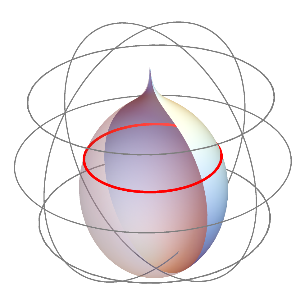
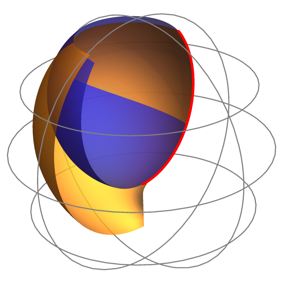
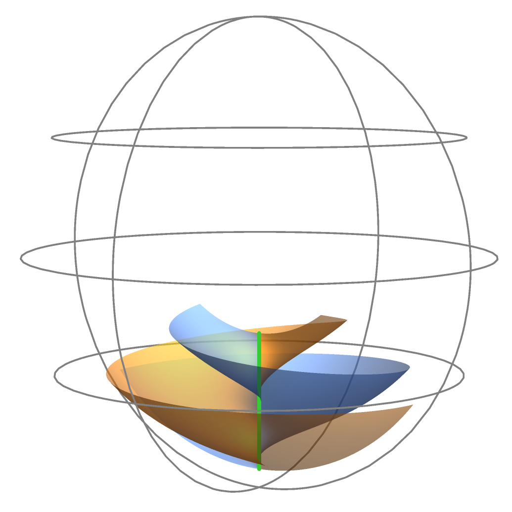
X^{\mathrm{E}}=\begin{pmatrix}e^{(a-2)v}&e^{2iu+av}\\ e^{-2iu+av}&e^{(a+2)v}\end{pmatrix}=R^{\mathrm{E}}(u)e^{av}\begin{pmatrix}e^{-2v}&1\\ 1&e^{2v}\end{pmatrix}R^{\mathrm{E}}(u)^{\star}

where $w=u+iv$ (see also Figure 1).

Refer to caption — Figure 1. Elliptic catenoids in $3$ -dimensional light cone with $a=\frac{3}{2}$ on the left, and $a=4$ on the right, where the initial given curve is highlighted.

4.2. Hyperbolic catenoids

Given a one parameter group of hyperbolic rotations

R^{\mathrm{H}}(u)=\begin{pmatrix}e^{u}&0\\ 0&e^{-u}\end{pmatrix},

the curve

\gamma(u)\mathrel{\mathop{\ordinarycolon}}=R^{\mathrm{H}}(u)\begin{pmatrix}1&1\\ 1&1\end{pmatrix}R^{\mathrm{H}}(u)^{\star}=\begin{pmatrix}e^{2u}&1\\ 1&e^{-2u}\end{pmatrix}

is a hyperbolic circle. Note that $\langle\dot{\gamma},\dot{\gamma}\rangle=4$ and that $\gamma(0)=\begin{pmatrix}1&0\\ 1&1\end{pmatrix}f_{3}\begin{pmatrix}1&0\\ 1&1\end{pmatrix}^{\star}$ .

To find the Björling data, we find that any $\mathcal{L}$ satisfying the conformality condition must take the form

\mathcal{L}_{\pm}(u)=f(u)\gamma(u)\pm f_{2},

for any function $f$ . Since $\mathcal{L}_{+}$ fails the orientability condition, we set $\mathcal{L}=\mathcal{L}_{-}$ . We also have that $\mathcal{L}$ is generated by the rotation under consideration; thus,

\mathcal{L}(u)=b\gamma(u)\pm f_{2},

for some constant $b$ .

Now, we calculate the Björling data as

G=\frac{b+2i}{b-2i}e^{2u},\quad\text{and}\quad\Omega=\frac{1}{8}(b-2i)^{2}e^{-2u}\operatorname{d\!}{u}.

Analytically extending $G$ and $\Omega$ and letting

\frac{b+2i}{b-2i}e^{2w}=z,

so that

G=z,\qquad\Omega=\lambda\frac{\operatorname{d\!}{z}}{z^{2}},\qquad\lambda=\frac{4+b^{2}}{16},

we can use Fact 4.2 to compute the explicit parametrizations for hyperbolic catenoid:

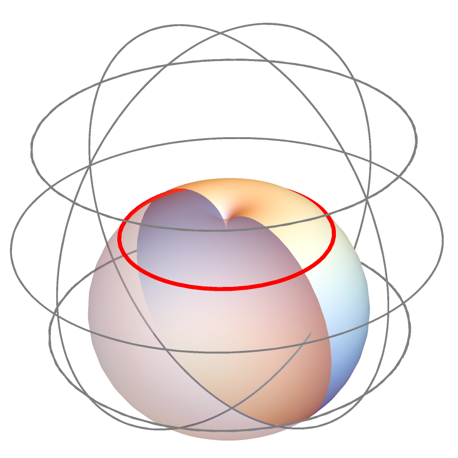
X^{\mathrm{H}}=\begin{pmatrix}e^{2u+bv}&e^{(b+2i)v}\\ e^{(b-2i)v}&e^{-2u+bv}\end{pmatrix}=R^{\mathrm{H}}(u)e^{bv}\begin{pmatrix}1&e^{2iv}\\ e^{-2iv}&1\end{pmatrix}R^{\mathrm{H}}(u)^{\star}

where $w=u+iv$ (see Figure 2).

4.3. Parabolic catenoids

Finally, we consider the parabolic rotation

R^{\mathrm{P}}(u)=\begin{pmatrix}1&u-1\\ 0&1\end{pmatrix}

applied to the point $\begin{pmatrix}1&1\\ 1&1\end{pmatrix}$ to obtain a parabolic circle

\gamma(u)=R^{\mathrm{P}}(u)\begin{pmatrix}1&1\\ 1&1\end{pmatrix}R^{\mathrm{P}}(u)^{\star}=\begin{pmatrix}u^{2}&u\\ u&1\end{pmatrix}.

Note that $\langle\dot{\gamma},\dot{\gamma}\rangle=1$ and that $\gamma(1)=\begin{pmatrix}1&0\\ 1&1\end{pmatrix}f_{3}\begin{pmatrix}1&0\\ 1&1\end{pmatrix}^{\star}$ .

We note that any $\mathcal{L}$ satisfying the conformality condition must satisfy

\mathcal{L}_{\pm}(u)\mathrel{\mathop{\ordinarycolon}}=f(u)\gamma(u)\pm f_{2}

for some function $f$ , and direct calculation tells us that $\mathcal{L}_{-}$ fails the orientability condition. Thus, we choose $\mathcal{L}=\mathcal{L}_{+}$ , and the fact that $\mathcal{L}$ must generated by the rotation under consideration allows us to deduce that

\mathcal{L}(u)=c\gamma(u)+f_{2}.

for some constant $c$ .

Using $\gamma$ and $\mathcal{L}$ as the Björling data, we calculate that

G=u+\frac{2i}{c},\quad\text{and}\quad\Omega=\frac{c^{2}}{4}\operatorname{d\!}{u}.

Analytically extending $G$ and $\Omega$ and making change of coordinates so that

w+\frac{2i}{c}=z,

we have

G=z,\qquad\Omega=\frac{c^{2}}{4}\operatorname{d\!}{z}.

This allows us to use Fact 4.3 to obtain explicit parametrizations for the parabolic catenoids:

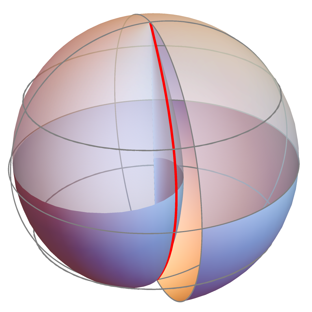
X^{\mathrm{P}}=\begin{pmatrix}e^{cv}(u^{2}+v^{2})&e^{cv}(u+iv)\\ e^{cv}(u-iv)&e^{cv}\end{pmatrix}=R^{\mathrm{P}}(u+1)e^{cv}\begin{pmatrix}v^{2}&iv\\ -iv&1\end{pmatrix}R^{\mathrm{P}}(u+1)^{\star}

where $w=u+iv$ (see Figure 3).

4.4. Classification of rotationally invariant zero mean curvature surfaces

Any circle in $\mathbb{Q}^{3}_{+}$ is congruent to one of the circles we constructed as orbits of points under rotations up to homotheties and isometries. Thus we conclude:

Theorem 4.4.

Any rotationally invariant zero mean curvature surfaces in $\mathbb{Q}^{3}_{+}$ must be a piece of one of the following surfaces (given with its respective Weierstrass data):

•

elliptic catenoid $(G=\frac{a-2}{a+2}e^{2iw},\Omega=\frac{-i(a+2)^{2}}{8}e^{-2iw}\operatorname{d\!}{w})$
•

hyperbolic catenoid $(G=\frac{b+2i}{b-2i}e^{2w},\Omega=\frac{(b-2i)^{2}}{8}e^{-2w}\operatorname{d\!}{w})$ , or
•

parabolic catenoid $(G=w+\frac{2i}{c},\Omega=\frac{c^{2}}{4}\operatorname{d\!}{w})$

up to homotheties and isometries of $\mathbb{Q}^{3}_{+}$ .

4.5. Additional example with analytic extensions

As in the parabolic catenoid case, let us take the parabolic circle as the initial curve, i.e.

\gamma(u)=R^{\mathrm{P}}(u)\begin{pmatrix}1&1\\ 1&1\end{pmatrix}R^{\mathrm{P}}(u)^{\star}=\begin{pmatrix}u^{2}&u\\ u&1\end{pmatrix}.

We have seen that $\mathcal{L}=f\gamma+f_{2}$ for any function $f$ satisfies both the conformality condition and the orientability condition.

Now, if we take

f(u)=\frac{c}{u}

for $u\in(0,\infty)$ , then we have $\mathcal{L}=\frac{c}{u}\gamma+f_{2}$ is not generated by the rotation under consideration; thus, the resulting surface will not be rotationally invariant. We can still calculate that

G=\frac{c+2i}{c}u,\qquad\Omega=\frac{c^{2}}{4u^{2}}\operatorname{d\!}{u}.

Analytically extending $G$ and $\Omega$ and letting

\frac{c+2i}{c}w=\mathrel{\mathop{\ordinarycolon}}z,

so that

G=z,\qquad\Omega=\lambda\frac{\operatorname{d\!}{z}}{z^{2}},\qquad\lambda=\frac{c(c+2i)}{4},

we can use Fact 4.2 to compute the explicit parametrizations:

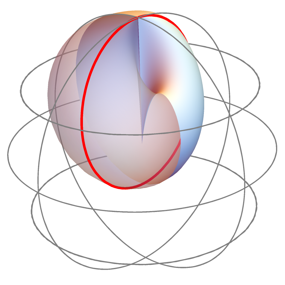
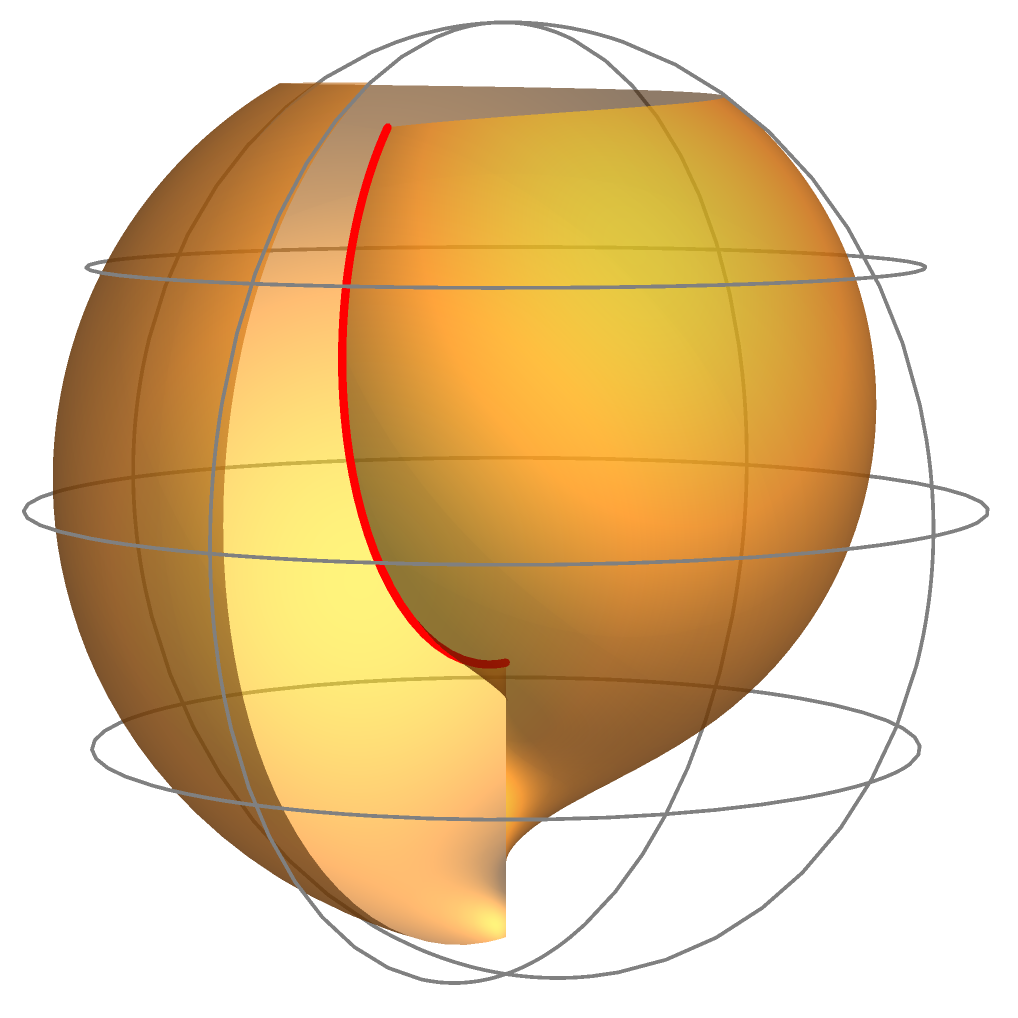
X=e^{cv}\begin{pmatrix}e^{2u}&e^{u+iv}\\ e^{u-iv}&1\end{pmatrix},

where $w=e^{u+iv}$ (see Figure 4).

If we change parameters so that $\tilde{u}=e^{u}$ , then we obtain

\tilde{X}=e^{cv}\begin{pmatrix}\tilde{u}^{2}&e^{iv}\tilde{u}\\ e^{-iv}\tilde{u}&1\end{pmatrix}

so that

\langle\tilde{X}_{v},\tilde{X}_{v}\rangle=e^{2bv}\tilde{u}^{2}.

This implies $L(v)\mathrel{\mathop{\ordinarycolon}}=\tilde{X}(0,v)$ is a lightlike curve in $\mathbb{Q}^{3}_{+}$ . In fact,

	$\displaystyle L(v)$	$\displaystyle=\tilde{X}(0,v)=\begin{pmatrix}0&0\\ 0&e^{cv}\end{pmatrix}$
		$\displaystyle=\begin{pmatrix}e^{\frac{-cv}{2}}&0\\ 0&e^{\frac{cv}{2}}\end{pmatrix}\begin{pmatrix}0&0\\ 0&1\end{pmatrix}\begin{pmatrix}e^{\frac{-cv}{2}}&0\\ 0&e^{\frac{cv}{2}}\end{pmatrix}^{\star}$
		$\displaystyle=R^{\mathrm{H}}(\tfrac{-cv}{2})\begin{pmatrix}0&0\\ 0&1\end{pmatrix}R^{\mathrm{H}}(\tfrac{-cv}{2})^{\star},$

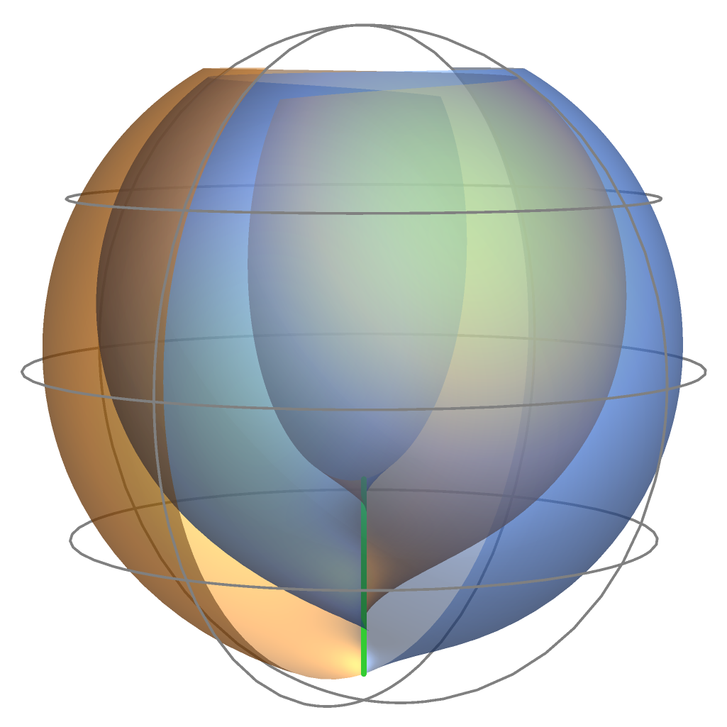
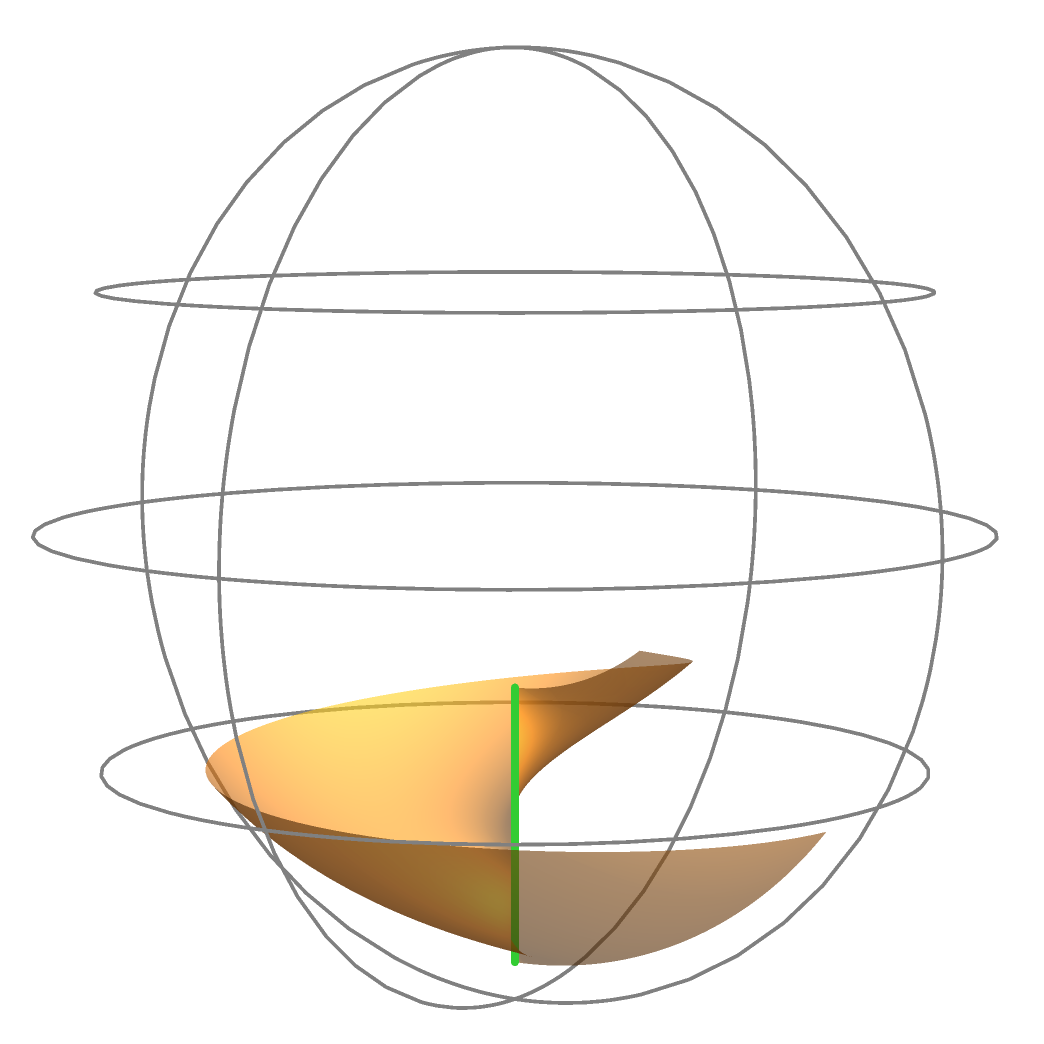
and thus $L$ is a lightlike circle. Therefore, we have that $\tilde{X}$ is an analytic extension of $X$ across the lightlike circle $L$ (see Figure 5).

Acknowledgements. The last author gratefully acknowledges the support from NRF of Korea (2017R1E1A1A03070929 and NRF 2020R1F1A1A01074585).

(3.8)	$\displaystyle\|\gamma_{11}\Lambda_{21}-\gamma_{21}\Lambda_{11}\|^{2}$	$\displaystyle=b^{2}+c^{2}+e^{2}+f^{2}+2(ce-bf)$
		$\displaystyle=\|\dot{\gamma}\|^{2}+\|\mathcal{L}\|^{2}+2(ce-bf)$
		$\displaystyle=2(\|\dot{\gamma}\|^{2}-(bf-ce)).$

Björling problem for zero mean curvature surfaces in the three-dimensional light cone

Abstract.

Key words and phrases:

2020 Mathematics Subject Classification:

1. Introduction

2. Preliminaries

2.1. Hermitian matrix model of three-dimensional light cone

2.2. Surface theory and Weierstrass-type representation

Fact 2.1.

3. Solution of the Björling problem

3.1. The conformality condition for the Björling data

Remark 3.1.

3.2. The orientability condition for the Björling data

Definition 3.2.

Lemma 3.3.

Proof.

Lemma 3.4.

Proof.

Lemma 3.5.

Proof.

Remark 3.6.

Remark 3.7.

Theorem 3.8.

4. Rotational zero mean curvature surfaces in ℚ+3\mathbb{Q}^{3}_{+}

Definition 4.1.

Fact 4.2 ([yang_bjorling_2017, Lemma 4.2]).

Fact 4.3 ([yang_bjorling_2017, Lemma 4.2]).

4.1. Elliptic catenoids

4.2. Hyperbolic catenoids

4.3. Parabolic catenoids

4.4. Classification of rotationally invariant zero mean curvature surfaces

Theorem 4.4.

4.5. Additional example with analytic extensions

References

4. Rotational zero mean curvature surfaces in $\mathbb{Q}^{3}_{+}$