Bipartite Leggett-Garg and macroscopic Bell inequality violations using cat states: distinguishing weak and deterministic macroscopic realism
Abstract
We consider tests of Leggett-Garg’s macrorealism and of macroscopic local realism, where for spacelike separated measurements the assumption of macroscopic noninvasive measurability is justified by that of macroscopic locality. We give a mapping between the Bell and Leggett-Garg experiments for microscopic qubits based on spin eigenstates and gedanken experiments for macroscopic qubits based on two macroscopically distinct coherent states (cat states). In this mapping, the unitary rotation of the Stern-Gerlach analyzer is realized by an interaction where is the number of quanta. By adjusting the time of interaction, one alters the measurement setting. We thus predict violations of Leggett-Garg and Bell inequalities in a macroscopic regime where coarse-grained measurements need only discriminate between two macroscopically distinct coherent states. To interpret the violations, we distinguish between different definitions of macroscopic realism. Deterministic macroscopic local realism (dMR) assumes a definite outcome for the measurement prior to the unitary rotation created by the analyser, and is negated by the violations. Weak macroscopic realism (wMR) assumes a definite outcome for systems prepared in a superposition of two macroscopically-distinct eigenstates of , after the unitary rotation. We find that wMR can be viewed as consistent with the violations. A model is presented, in which wMR holds, and for which the macroscopic violations emerge over the course of the unitary dynamics. Finally, we point out an EPR-type paradox, that a weak macro-realistic description for the system prior to the measurement is inconsistent with the completeness of quantum mechanics.
I Introduction
Bell’s theorem constrains the predictions of all local hidden variable theories to values governed by inequalities bell-brunner-rmp ; CShim-review ; Bell-2 ; det-bell . These inequalities can be violated by quantum mechanics, giving a falsification of both local realism and local causality. Bell tests involve measurements made on two separated particles, performed on timescales such that the two measurement events are spacelike separated. At each location, there is a choice between two measurement settings. To date, almost all Bell tests have examined microscopic systems. Bell violations have been predicted for large numbers of particles meso-bell-higher-spin-cat-states-bell ; cv-bell ; cat-bell ; mdr-mlr ; macro-bell-additional ; cv-bell-macro-ali , but, in almost all cases, the measurements for one of the settings require a resolution of a few particles, or at the level of Planck’s constant.
By contrast, Leggett and Garg derived inequalities that do not require such fine resolution of measurement legggarg-1 . Leggett-Garg inequalities are designed to falsify the assumption of macrorealism (M-R) for systems that at certain times are in a superposition (e.g. ) of two macroscopically distinct states s-cat-1 . M-R combines two premises: Macroscopic realism (MR) asserts that the system must actually be in one or other of those two states at the given time. The second premise, macroscopic noninvasive measurability (NIM), asserts the existence of a measurement that can distinguish between the two macroscopic states, with negligible effect on the subsequent dynamics (at a macroscopic level). Macroscopic realism implies a predetermined value for the outcome of the measurement legggarg-1 . Since the two states and can be distinguished by a measurement allowing a macroscopic uncertainty, the hidden variable need not specify the results of measurements to a resolution of . This was recognised by Leggett and Garg who assigned the values for the two outcomes of , in order to derive inequalities legggarg-1 .
Leggett-Garg inequalities have been reported violated for a wide range of systems emary-review ; jordan_kickedqndlg2-1 ; weak-solid-state-qubits ; NSTmunro-1 ; massiveosci-1-1 ; manushan-cat-lg ; weak-hybrid ; leggett-garg-recent ; macro-bell-lg ; nst . A complication for the interpretation of the violations has been the justification of the NIM premise for practical measurements leggett-garg-recent . Different strategies are used, including (in a recent macroscopic superconducting experiment) a control experiment which quantifies the amount of disturbance induced by the measurement, if the system is indeed in one of the states or NSTmunro-1 . An alternative strategy (that does not assume the system to be in one of the fully specified quantum states) is to violate bipartite Leggett-Garg or macroscopic Bell inequalities macro-bell-lg ; weak-hybrid ; cv-bell-macro-ali . Here, the NIM premise is replaced by that of macroscopic locality. Recent work gives predictions for such violations using NOON and multi-component cat states macro-bell-lg . The question becomes how to interpret such violations. In particular, we ask whether the assumption of the macroscopic hidden variable for the coarse-grained measurement can be negated.
In this paper, we give full details of the results presented in the Letter letter , which analyses this question. To facilitate the analysis, we give predictions of violations of macroscopic Bell inequalities and of bipartite Leggett-Garg inequalities for the conceptually simple case where a system at certain times is found to be in a superposition of two macroscopically distinct coherent states, and (cat states), as . Similar to the results of Ref. macro-bell-lg , the violations are obtained using only measurements which discriminate between the two coherent states, thereby allowing macroscopic uncertainties.
In order to interpret the violations, we are first careful to define macroscopic realism in the weakest (i.e. most minimal) sense, as weak macroscopic realism (wMR), the premise that a macroscopic hidden variable specifies the outcome of the coarse-grained pointer measurement . In contrast to many previous macrorealism tests, we find it is not necessary to include in the definition of macroscopic realism that the system be in one or other of two specific quantum states (e.g. and ), or even that the system be in one or other of two unspecified quantum states. The violations given in this paper therefore provide strong tests of both macrorealism (M-R) and macroscopic local realism (MLR), and also of macroscopic local causality (MLC).
In this paper, we further weaken the definition of weak macroscopic realism, by specifying to be a pointer measurement, and the distinct states and to be states with a definite outcome for the (coarse-grained) . In other words, the assumption of wMR asserts the validity of the macroscopic hidden variable for the state prepared after a unitary transformation that determines the choice of measurement setting. We show that the violations of M-R and MLR/ MLC given in this paper can be viewed consistently with wMR.
On the other hand, we show that the violations falsify deterministic macroscopic realism (dMR), which specifies well-defined values prior to such a unitary transformation. The assumption of dMR also includes the assumption of macroscopic locality (ML), which states that the value of cannot be changed by spacelike separated measurement events at another site. The premise of dMR implies the validity of two hidden variables, and , ascribed to the system simultaneously (prior to ) to predetermine the outcome of two pointer measurements, and , and is negated by the violation of the macroscopic Bell inequalities.
We find that the consistency of the violations with wMR is possible because of the unitary dynamics associated with the choice of measurement setting. The unitary rotation that determines the measurement setting transforms the system from one pointer superposition to another, over a time interval . The system is therefore not considered to be in a superposition of eigenstates of both pointer measurements, and , simultaneously. In our analysis, the transformation that determines the measurement setting is given by a nonlinear Hamiltonian where is the mode number operator. The dynamics leading to the macroscopic violations can therefore be observed over the interval . Recent work predicts violations of Bell inequalities at a microscopic level for the dynamical trajectories of two entangled particles bell-trajectories . This is consistent with our conclusion that deterministic macroscopic realism fails, since the choice of measurement setting involves dynamics, as given by .
There are open questions. While we show consistency with wMR, the results of this paper neither falsify nor validate this premise. The validation of this premise might be expected, in view of the known emergence of classicality with coarse-grained measurements coarse-3 ; coarse-peres ; kofler-bruck-leggett-garg-coarse . The concept might also be consistent with recent proposals to interpret quantum mechanics using theories based on multiple interacting classical worlds mhall , or with an epistemic restriction of order Planck’s constant budiyono ; bartlett-gaussian ; macro-pointer ; q-trajectories-drummond , and may also be consistent with recent interpretations of the double-slit experiment double-slit-Aharonov .
However, it is clear from the violations of the Leggett-Garg inequalities presented in this paper (and elsewhere) that if wMR holds, then the dynamics associated with the macroscopic hidden variables cannot be given by classical mechanics. If wMR holds, we show for the tests of this paper that the violations of the Leggett-Garg inequalities would therefore arise from the breakdown of the NIM assumption. We explain how this breakdown arises (in the bipartite model) from quantum nonlocality, the new feature being that there is a macroscopic nonlocality (associated with macroscopically distinct qubits and ), which we show emerges over the timescales associated with the unitary interactions at both sites. While the distinction between predictions for the superposition and the classical mixture of the two macroscopically distinct states is negligible (of order ), a macroscopic difference emerges over the course of the dynamics corresponding to the unitary rotations.
From an alternative point of view, we summarise in this paper that if one does postulate the validity of wMR, then inconsistencies arise. This can be shown in the form of an EPR-type paradox epr-1 , similar to that given in earlier papers macro-coherence-paradox ; eric_marg-1 ; irrealism-fringes ; macro-pointer . If one assumes wMR, then the assumption that the system is in one of two quantum states, such as or , can be negated. Hence, wMR is inconsistent with the completeness of quantum mechanics, which gives predictions at the level of .
Layout of paper: The paper is organised as follows. In Section II, we review and extend previous work to give derivations of bipartite Leggett-Garg and macroscopic Bell inequalities. The macroscopic Bell inequalities are derived assuming deterministic macroscopic (local) realism or macroscopic local causality, both of which are negated by violations of the inequalities given in this paper.
In Section III, we demonstrate a mapping between the spin- Bell experiments performed on microscopic qubits and , and a gedanken experiment performed on macroscopic qubits, and . The unitary rotation of the polariser or spin analyser is mapped to a transformation , which is realized for and by an evolution at certain times manushan-cat-lg . We thus show that macroscopic Bell inequalities are violated for spacelike separated systems, and , prepared in an entangled two-mode cat state . The mapping relies on the orthogonality of the coherent states, which strictly holds only for , . In our explicit model, we give full calculations, and compute the values of and for which experiments could be performed.
In Section IV, we predict violations of Leggett-Garg’s macrorealism, for both single and bipartite cat-state systems, following along the lines of Ref. manushan-cat-lg . In the Bell test, the angle is the measurement setting. In the Leggett-Garg test, the angle gives the time of evolution between measurements made at different times. The dynamics associated with the unitary evolution can be visualised by plotting the function Husimi-Q-1 . We explain weak macroscopic realism (wMR) in Sections III.E and also in Section VI. Evaluation of the function dynamics is given in Sections III.D and IV.B.2.
In Section V, we examine the measurement process more carefully. For the bipartite Leggett-Garg test, whether the measurement is performed or not on system is determined by the duration of unitary evolution, at the second location . By contrast, the timing of the final irreversible (“collapse”) stage of the measurement at is unimportant. We show by calculation that whether the collapse occurs before or after the subsequent evolution at is irrelevant to the violations, making only a difference of order to the final probabilities. Here we point out that although the results of this paper are consistent with weak macroscopic realism (wMR), it is possible to establish inconsistencies with quantum mechanics, similar to an EPR-type paradox. Finally, a conclusion is given in Section VI.
II Macroscopic Bell and bipartite Leggett-Garg inequalities
We first outline and extend the Bell and bipartite Leggett-Garg inequalities for a macroscopic system, as proposed in Refs. weak-hybrid ; macro-bell-lg . In order to test macroscopic realism, we combine aspects of the original Bell and Leggett-Garg proposals. As with Bell’s proposal, there are two spatially separated systems and upon which local measurements are made. Similar to the Leggett-Garg proposal, the systems at each location evolve dynamically according to a local Hamiltonian (or ), so that measurements can be made at different times. The measurements at each site and give only two possible outcomes, corresponding to two macroscopically distinguishable states. The outcomes are designated as pseudo-spins, and , respectively.
In fact, we present two types of test of macroscopic realism. The first (Section II.A) is a macroscopic Bell test, where for a given run of the experiment, one makes single measurements at each site, and . For each measurement, there is a choice between two measurement settings, corresponding to a choice between two different times of interaction with a measurement device. The second type of test of macroscopic realism (Section II.B) is similar to that proposed by Leggett and Garg, except there are two sites. In a given run of the experiment, one makes sequential measurements at different times , on the systems at the separated sites, and .

II.1 Macroscopic Bell test
II.1.1 Deterministic macroscopic (local) realism
We consider the situation of Figure 1. One prepares the state of the system at a time . At each site there are two possible measurement settings ( and at , and and at ) and for each of these measurements there are only two outcomes, corresponding to states of the system that are macroscopically distinct. We refer to the outcomes and as “spin” outcomes, and label the measurements at sites and as and respectively. Distinguishing only between macroscopically distinct outcomes, the measurements and can allow a significant error, beyond the level of as we will show by example in Sections III and IV. As such, we refer to the measurements as coarse-grained, or macroscopic, measurements.
The assumption of macroscopic realism (MR), as specified by Leggett and Garg legggarg-1 , asserts that each system prior to the measurement and is in one or other of the two macroscopically distinguishable states, which have a definite outcome for the spin. Here, we do not wish to restrict that the two macroscopically distinct states are specific states, and , or even that they are quantum states. The definition of MR is generalised to postulate that prior to the measurement and , the system is in a state for which the outcome of the macroscopic, coarse-grained measurement or is definite, being either or . Assuming MR, macroscopic hidden variables and with values or can be ascribed to the systems and at the time immediately prior to the measurement, the values giving the predetermined outcomes for the measurements and respectively. These variables, introduced by Leggett and Garg, are hidden variables, since they are not explicitly given by quantum mechanics.
If there is a choice of measurement settings and at a given site, then one assumes (based on the assumption of MR) that two hidden variables and describe the state of the system as it exists prior to the time the choice is made, to predetermine the results of both measurements, and . Similar to the original Bell derivation Bell-2 ; det-bell , we call the definition of MR as given here deterministic macroscopic realism (dMR).
Assuming locality, that the value of the macroscopic hidden variable for the system at one site cannot be changed by the local measurement at the other site bell-brunner-rmp ; CShim-review ; Bell-2 ; det-bell , it is straightforward to derive the Clauser-Horne-Shimony-Holt (CHSH) Bell inequality, , where CShim-review
| (1) |
Here and ( and ) are two measurement settings at sites A (and B) respectively, and is the expectation value for the product , for the choice of settings, and . The combined assumptions of locality and deterministic macroscopic realism are referred to as deterministic macroscopic local realism (MLR), or simply deterministic macroscopic realism, as the condition of locality is naturally implied by dMR for two sites det-bell . The derivation of (1) follows from the assumption of MLR, which implies .
The local measurements and have two stages: a unitary stage for which there is an interaction with an analyzer device, and a final stage which includes an irreversible coupling to a reservoir i.e. to a detector. The unitary stage determines the measurement setting, and is analogous to the transmission of a photon or spin- particle through a polarizing beam splitter or Stern-Gerlach analyzer. Thus, in the traditional Bell tests, and are polarizer or analyzer angles, determining the direction of polarisation or spin that is to be measured at each site. The final pointer stage corresponds to detection in one of the arms of the polarizing beam splitter.
For the examples given in this paper, following Refs. macro-bell-lg ; manushan-cat-lg , the unitary stage of the measurement at each site comprises an interaction with a nonlinear medium, and the measurement setting is determined by the time duration of the interaction. This need not be a choice of time itself, but can instead be a choice of the degree of nonlinearity of the medium, the choice of measurement setting being made by a switch. We identify at each site two choices of times for the measurements: and ( and ) at (and ) respectively. The Bell inequality (1) becomes where
| (2) |
Modelling the measurement in this way as an interaction with a device emphasises that the measurement will occur over a finite time interval. To justify the locality assumption, it is assumed that the measurement events at each site are spacelike separated.
II.1.2 Macroscopic local causality
When deriving (1) and (2), it is assumed that two macroscopic hidden variables describe each system at the time immediately prior to the measurement () bell-brunner-rmp ; CShim-review ; Bell-2 ; det-bell . These are and for system , and and for system . Each of these variables assumes values or . Thus, the system at is in a state with simultaneous predetermined values for the measurements and , and similarly for .
However, it is well known that the Bell inequality (1) can be derived with a weaker assumption allowing for a stochastic interaction with a local measurement device det-bell ; CShim-review . Here, one assumes that the system at time is in a hidden variable state given by a set of hidden variables with probability density . One defines the probability for obtaining a spin outcome or at site , given the system prior to measurement is in the state and given the choice of measurement setting for the local device at . The probability is defined similarly, for the spin outcome at , given the measurement setting for the local measurement device at . The locality assumption is that probability does not depend on , and does not depend on . These assumptions can be viewed as a single assumption, local causality det-bell .
Thus, the Bell inequalities (1) and (2) follow from a weaker assumption, that we refer to as macroscopic local causality (MLC). The assumption is similar to local causality, except here one postulates that prior to the measurement, the system is in a hidden variable state which gives a definite probability for just two macroscopically distinct outcomes. In this paper, the Bell inequalities can be derived from either MLR or MLC, and we will use MLR to imply either definition.
II.2 Bipartite Leggett-Garg tests
The Leggett-Garg inequalities were derived for the situation where one considers succcessive measurements on a single system, at times . Here, following macro-bell-lg ; weak-hybrid and different to the original treatment legggarg-1 , we consider two systems and (Figure 2). Measurements and are made on systems and at times and respectively. The measurements give two outcomes, and , corresponding to two macroscopically distinguishable states. However, here there is no choice of measurement setting at a given time: Rather, the unitary rotation stage (or ) of the measurement is considered to be part of the dynamics. In the examples we consider in this paper, the measurements and that occur at the times and are analogous to the pointer measurements, and , of Figure 1.
The Leggett-Garg inequalities are derived based on the assumption of macroscopic realism legggarg-1 . Hence one may identify specific macroscopic hidden variables and to describe the states immediately prior to the pointer measurements and . Different to the Bell derivation of Section II.A.1 however, one does not ascribe to the system simultaneously at a time predetermined results and for both future measurements, and . What was the local unitary interaction ( or ) with the measurement device in the Bell test is now the local trajectory. One therefore assumes macroscopic realism for a measurement with just a single setting, at the time . This means that the Leggett-Garg-Bell inequalities for the systems of interest may be derived based on the assumption of weak macroscopic realism (wMR): that for a system prepared in a superposition of macroscopically distinct pointer states, the system can be described by a single hidden variable at that time (and this is not affected by a space-like separated measurement event at the different site ).
The traditional Leggett-Garg test invokes a second assumption, that it is in principle possible to determine which of the two macrosopically distinct states the system is in at any given time, by performing a noninvasive measurement that has a negligible effect on the subsequent dynamics legggarg-1 . This assumption is necessary because the traditional Leggett-Garg tests involve measurements at different times performed on the same system, and there is the possibility of direct disturbance of the system due to measurement. In this paper, we follow macro-bell-lg , and consider two systems (Figure 2). One assumes validity of (weak) macroscopic realism, but the additional assumption of noninvasive measureability is replaced by the assumption of locality. Specifically, for measurements at and that are spacelike separated events, one assumes the hidden variable value is not changed by whether the measurement at takes place or not, and similarly for .

We consider measurements made at times and at site , and at times and at site , where . Let us denote the spin outcome at for the measurement made at time by . The spin is defined similarly, for site . With the assumptions of macroscopic realism and noninvasive measurability (locality), the Leggett-Garg-Bell inequality
| (3) | |||||
where can be shown to hold legggarg-1 . This inequality was derived as a Leggett-Garg inequality in Ref. legggarg-1 , and as a Leggett-Garg-Bell inequality, in Refs. macro-bell-lg ; weak-hybrid . Since the expectation values of the inequality involve measurements made at diffferent sites, the inequality follows based on the assumption of locality, which justifies that . We note that while we assume the time order , in fact because we have two localised sites, we need only take and .
A three-time Leggett-Garg-Bell inequality
| (4) |
where is also useful. This is based on the original three-time Leggett-Garg inequality, derived for the single-system set-up, in Refs. weak-solid-state-qubits ; jordan_kickedqndlg2-1 . Here, one assumes however that a measurement at time at site does not affect the outcome at the later time at the same site, which raises the issue of a disturbance due to the measurement at . However, for correlated initial states, one may use that the result for can be inferred from a measurement of . Thus, assuming locality, one may deduce macro-bell-lg :
| (5) |
We note that the no-signalling-in-time (NSIT) equality has been shown to give a stronger test of Leggett-Garg’s macrorealism NSTmunro-1 ; nst . However, it is more challenging to use this equality for a bipartite test.
II.3 Summary of assumptions
Since we are to show violation of the macroscopic Bell and Leggett-Garg-Bell inequalities, it is important to summarise what is the weakest (i.e. minimal) assumption needed to derive the inequalities. The Bell inequalities (2) can be derived from the minimal assumption of macroscopic local causality (MLC), as in Section 1.A.2. In this paper, however, we use the terms macroscopic local realism (MLR) and macroscopic local causality (MLC) interchangeably. The Leggett-Garg-Bell inequalities (3) and (4) on the other hand are derived assuming weak macroscopic realism, combined with macroscopic noninvasiveness (NIM) of the measurement, which for two sites is justified by macroscopic locality (ML).
III Violating the macroscopic Bell inequalities
We consider the system of Figure 1 prepared in the initial “cat” state cat-bell-wang-1
| (6) |
Here and are coherent states for two modes, labelled and , and for convenience we assume , to be real and positive. We will ultimately take , . The normalisation constant is . In the limit where , are large, we note that and become orthogonal, and similarly and , so that . In this limit, we may write the cat state as a macroscopic two-qubit state
| (7) |
Here and are orthogonal states giving an outcome of and respectively, for a measurement of the sign of the coherent amplitude, . Similarly, and are orthogonal states, with outcome and for the measurement of the sign of the amplitude . The two modes and are spatially separated, being located at sites and , respectively. The sign of the coherent amplitude is taken to be the value of the “spin” for each mode (site).
III.1 Bell violations using unitary local transformations
At locations and , we assume local unitary transformations and take place, as in Figure 1. States and are transformed after a time and according to (at site )
| (8) |
and (at site )
| (9) |
For a system prepared in the superposition of eqn. (7), the system will evolve into the final state
| (10) |
where we have abbreviated and Using that the states are orthogonal, and defining the measurement which measures the sign (which we label as its “spin”), according to and , we find that the expectation value of the spin product is
| (11) |
For the traditional Bell experiment where the transformation is achieved using a polarising beam splitter, we have and , and
| (12) |
It is known that the choice of angles , , and in the Bell inequality (1) will lead to which violates the inequality.
III.2 Unitary transformations via nonlinear media
Now we consider how to realise the transformations (8) and (9). We seek a unitary transformation such that at site the transformation
| (13) |
holds, for the particular angle choices and . At site , we seek a transformation such that
| (14) |
for the angle choices , and . We drop subscripts and , where the meaning is clear.
These transformations can be achieved by interacting each single mode system with a nonlinear medium at the given site, where the interaction Hamiltonian is ( and even) manushan-cat-lg ; yurke-stoler-1 ; wrigth-walls-gar-1 ; macro-bell-lg . Here is the mode number operator and is the nonlinear coefficient. We choose units such that . The interaction takes place independently for each mode and , and we denote the respective Hamiltonians as and . Thus we define local interactions at each site
| (15) |
The boson destruction mode operators for modes and are denoted by and , respectively, and the number operators are and .


One may solve for the dynamics given by . If the system is prepared in a coherent state , the state after time is yurke-stoler-1
| (16) | |||||
where and . For an initial coherent state at , the state after a time is given similarly, as where . These solutions are well known manushan-cat-lg ; yurke-stoler-1 and are depicted graphically in Figures 3 and 4 in terms of the function, defined as Husimi-Q-1 . Here and is a coherent state. At certain intervals of time, the system evolves into a superposition of the macroscopically distinct coherent states and (Figure 4).
Suppose at time , the systems are in the initial states and . After a time , the system at is in the state (second picture of Figure 3). This gives the transformation of eq. (14) with manushan-cat-lg . We write the state at this time as
After a time , the state is which corresponds to the transformation eq. (13) with . We write the state at as manushan-cat-lg
| (18) |
To obtain the transformation (14) with , we consider the state at time manushan-cat-lg , which is given by . The state at the time is
These transformations are shown graphically in Figure 3. The transformations at each site and are summarised as
| (20) |
where , , and . Noting from above, , and .
The Bell test of Section III.A requires a measurement of the spin for the states after the unitary rotations. As we have seen above, the unitary parts of the measurements and are to be made by interacting with the nonlinear medium at each site. This creates the superpositions (LABEL:eq:state3-20) of the coherent states and ( and ) which are rotated relative to the initial state (). The initial states determine the orientiation of real axis (i.e. the phase direction). The coherent states and ( and ) are hence the basis states for a particular pointer measurement, () that determines the sign of the coherent amplitude i.e. the value of the macroscopic qubit. The pointer measurements are hence measurements of the quadrature phase amplitudes yurke-stoler-1
| (21) |
on the evolved states at each site. The orientation of the axis that defines quadratures is aligned with the orientation of the initial coherent states () in phase space. This is set in the experiment by a local oscillator. Finally, such a measurement involves a coupling to detectors. Let us denote the results of the pointer measurements and by and respectively. The final spin outcome of the measurement is taken to be if , and otherwise. Similarly, the outcome of the measurement is if , and otherwise.
III.3 Macroscopic Bell violations
At each site and , the system of Figure 1 prepared in the cat state (6) undergoes unitary transformations and , given by (20). There is the choice of two rotation angles, corresponding to two different times, at each site. These give transformations of the form (13) and (14).
A violation of the Bell inequality (1) is obtained if we select angles and at site , and and at site (Figure 1). Therefore, in order to violate the Bell inequality (2), we select (which gives rotation ) and (which gives rotation ). Similarly at site B, we select (rotation ) and (rotation ). Using the prediction given by (12) for orthogonal states undergoing the unitary transformations (8) and (9), we see that this choice of time-settings will give a violation of the Bell inequality (2).

To account for the nonorthogonality due to finite amplitudes and , we evaluate the distributions for the outcomes of the joint measurement of the amplitudes and (eqn (21), for each of the time-settings. This constitutes the prediction for the final pointer measurements. The final state after the unitary transformations is
where the unitary operators are given by (20) and is the normalisation constant. The probability is
| (23) |
where , are eigenstates of and respectively. Details of calculation are given in the Appendix. Integrating gives the results needed for the evaluation of the Bell inequality term, , of eqn (2). We use where
| (24) |
and , and are defined similarly for the remaining three quadrants.
The results for the four choices of time settings are shown in Figures 5 and 6. For , the overlap of the coherent states and (and and ) is small and there is agreement with the calculations based on the assumption of orthogonality of the states. For each time setting, the results of the measurements and have two possible values, and , and there are four joint outcomes. In Figure 5, the plots of show four distinct Gaussian peaks corresponding to the probabilities of these joint outcomes, the peaks becomes macroscopically separated for large and . We thus verify that maximal violations of the Bell inequality (2) () are indeed predicted for the macroscopic qubits, where measurements distinguish macroscopically distinct states, as , .


III.4 Dynamics of the unitary part of the measurement
In the set-up of Figure 1, two spacelike separated systems display failure of macroscopic local realism. As the measurements take place, the systems evolve dynamically over an interval of time. This is a realistic model because the analyser measurements involve interactions over a finite time duration. In order to gain insight into how the macroscopic Bell violations arise over the course of the dynamics, we present plots in terms of the Q function.
The Husimi Q function is defined uniquely as a positive function for a two-mode quantum state by where and are coherent states for the modes Husimi-Q-1 . It is a function of four real variables , , and , where and . The Q function is a quasi-probability distribution, corresponding to an anti-normal ordering of moments, and therefore (different to a positive Wigner function) does not provide a probability distribution for the actual outcomes , , of the measurements , . However, the function provides at any given time the correct probability distribution for the outcomes of the macroscopically separated spins and , as we confirm below.


Assuming the system is prepared in the cat state (6), the state of the system after interaction times at site and at site is given by eq. (LABEL:eq:234-1-1-1). The Q function at the time and is . The marginal for the two quadratures, given by
| (25) |
One can also evaluate the marginals for each system e.g. ) by integrating over and .
In Figures 7 and 8, we plot the marginals and corresponding to the states created after the interaction times and , as in Figure 5, where there is a violation of the Bell inequality (2). As expected, there is similarity in the macroscopic limit of the Q function with the actual distributions , of Figure 5. The additional noise of order (scaled to order in the plots) which is characteristic of the Q function does not change the probabilities for the macroscopically distinct outcomes, and .


To investigate the dynamics leading to the violation of macroscopic local realism (MLR), we give a comparison with the predictions if the system is initially prepared in the non-entangled mixed state
The mixture evolves to
We plot the Q function of the mixed state , eqn. (LABEL:eq:mixunit), in Figure 7 (lower) for the choice of time-settings that for the state lead to a violation of the Bell inequality (top). The mixed state has the interpretation that the system is in one or other of the quantum states with a definite outcome for and at a time , as , . Consistent with that interpretation, the dynamics does not lead to a violation of the Bell inequality. We see that the Q functions for the initial states ( and ) at are indistinguishable. In fact, calculation shows that there is a microscopic difference , of order , between these two Q functions. We also see that the Q functions arising from initial states ( and ) are indistinguishable if either or is zero. However, for the time settings where there is evolution (rotation) at both the sites, the final outcomes are macroscopically different.
The timescales of the dynamics leading to the violation of macroscopic local realism (MLR) can be visualised if we calculate the full dynamics associated with the unitary measurements (rotations) (Figures 9 and 10). The predictions for the joint distributions depend only on the absolute value of the times and of interaction with the measurement apparatus at each site. The same violation of the Bell inequalities can thus be achieved in different ways relative to a shared clock. For example, one may measure system first, and subsequently measure system ; or vice versa. Alternatively, one may measure by evolving the systems simultaneously. In Figures 9 and 10, we choose to evolve sequentially, with first. On comparing the sequences of Q functions for the entangled state and for the mixture in Figures 9 and 10, we observe the transition from indistinguishable Q functions at though to a small but noticable difference at times and . Finally, at times and , the difference has become macroscopic.
To understand why there is little distinction between the results for and if the unitary evolution acts on the state at one site only (), but not where for and , we calculate the probabilities for each case, in the Appendix. The difference arises from quantum interference terms damped by in the first case but which are not damped for the entangled state for certain values of , in the second case. The effect for large and is in direct analogy with the calculations given for the two-qubit Bell experiment in Section III.A, as expected since these calculations rely on the orthogonality of the states forming the qubit.
The plots in Figure 8 show the marginals and at each site. These plots highlight the two-state nature of the systems immediately after the unitary rotations and for the choice of measurement settings required for the Bell violation. Identical two-state plots are obtained for the coarsely selected times given in Figure 9 that show the dynamics during those measurements. However, as seen from Figure 4, over very much shorter time scales, the unitary dynamics involves a continuous transition, and the systems cannot be regarded as two-state systems at all times.
III.5 Conclusions
It is clear from the summary given in Section II.C that the violations predicted for the macroscopic Bell inequality (1) and (2) imply failure of deterministic macroscopic (local) realism (dMR) and macroscopic local causality (MLC), which we collectively refer to as macroscopic local realism (MLR). We explain that there is no inconsistency however with the assumption of weak macroscopic realism (wMR), as introduced in the Sections I and II.
The peaks of the Q function in the Figures give the values for the probabilities of the macroscopically distinct outcomes ( and ) for the spins, and . The description is of an entire ensemble, not of an individual system. Therefore the negligible difference of order between the Q functions of the classical mixture (eqn (LABEL:eq:mixqstate)) and the superposition (eqn (6)) refers to the average over many identically prepared systems, not to any individual system at any given time.
In what we refer to here as the weak macroscopic realism (wMR) model, an interpretation is given that goes beyond this. Consider the cat-state , which for large is a superposition of two states with definite and macroscopically distinct outcomes for the pointer measurement () of the spins (). Similar superpositions (10) are created after the unitary rotations at each site, as evident in Figures 7 and 9. In analogy with the polarising beam splitter or analyser in a Bell experiment, brings about a change of basis, in preparation for a pointer measurement. The Q function for such superposition states gives macroscopically distinct peaks corresponding to outcomes () for ().
The wMR interpretation is that immediately prior to the measurement at each site, the local system was in one or other of two states (referred to as and ) predetermined to give one or other of the macroscopically distinguishable outcomes or respectively. This assumption is defined in parallel with that of macroscopic locality of the pointer (MLP): that the measurement at does not affect the (macroscopic) spin outcome at (and vice versa). In this model, the violation of macrorealism and of macroscopic local realism arises over the course of the unitary dynamics. The distinction between predictions for the initial Bell superposition and a classical mixture of the two pointer eigenstates is quantified by terms of order . The violations of macro-realism and MLR emerge with the amplification of the effect of , over the course of the unitary dynamics corresponding to the rotation of basis.
In this interpretation, it is not assumed that the states and correspond to and , nor that and correspond to quantum states (indeed, they cannot, as shown in Section V). Nonetheless, the wMR model asserts the predetermination of the macroscopic prediction.
IV Leggett-Garg tests of macro-realism and macroscopic local realism
In this section, we propose tests of macrorealism and of macroscopic local realism using cat states and the Leggett-Garg inequalities. For measurements of spin made on a single system at consecutive times , macrorealism implies the Leggett-Garg inequality weak-solid-state-qubits ; jordan_kickedqndlg2-1
| (28) |
IV.1 Leggett-Garg test with a single system
We first outline the approach using a single system, but as applied to the cat states. Here, we follow an analysis similar to that given by Ref. manushan-cat-lg . The system is prepared at time in a coherent state . The spin if measured at this time gives the result . The result however is known deterministically, from the preparation. Following preparation, there is evolution according to the Hamiltonian of eqn (15), for a time . This gives the state
| (29) |
At the time , after the rotation, we may choose to measure the value of the spin . This gives . If not measured, the system continues to evolve according to until the time . The state of the system at is
| (30) |
which implies .
To test the Leggett-Garg inequality, one requires to evaluate . Here, one assumes macrorealism. We follow the usual approach, and suppose that an ideal measurement of takes place at time , which would give a result of either or . If the result is , then one assumes the system was in the state at the time , based on the assumption that the measurement did not disturb the system, and noting that tomography of the (average) state conditional on the result would be consistent with the quantum state For either state , one deduces , since the system evolves for a further time . Thus, the prediction is . Overall, the value for the left-side of the Leggett-Garg inequality (28) is , which violates the Leggett-Garg inequality.
A criticism of the above approach is that there is a change due to the measurement at time , and the state prior to the measurement was different to . However, macrorealism postulates the existence of an ideal measurement where any such effect will have negligible impact on the future dynamics, as the system becomes macroscopic (). This would not change the prediction of a violation, if macrorealism is correct.
The dynamics as depicted in terms of the Q function is given for the sequence of times in Figure 11. There are two cases to compare: whether a measurement is performed at time , or not. Details are given in the Appendix. The lower sequence plots where a measurement is performed at time , assuming that for the ideal measurement this is done in such a way to instigate a collapse into one or other of the coherent states, as above. The Q functions (LABEL:eq:q2-2) and (48) describe the states for an ensemble of systems immediately after the time , if a measurement has or has not taken place at time respectively. The two Q functions differ by the term
| (31) |
This term is negligible for even moderate and there is no distinguishable difference between the functions at the time (refer Figure 11). Despite the negligible difference between the (average) states at time , the states at time are macroscopically different. The Q function model is consistent with the Leggett-Garg premise that a measurement exists which has increasingly negligible effect on the immediate state of the system as the system becomes larger legggarg-1 . This is because is proportional to . In this model, the Leggett-Garg inequalities are violated because the small effect nonetheless impacts the future dynamics at a macroscopic level.


A challenge for testing macrorealism is to overcome the criticism that the ideal measurement cannot be realised. While arguments can be made that the system at was in a state sufficiently close to or , if macrorealism is correct NSTmunro-1 , it becomes difficult to exclude that the system, in a theory alternative to quantum mechanics, is described by some other state at time , prior to measurement. This motivates the next section.
IV.2 Bipartite Leggett-Garg tests
IV.2.1 Violation of inequalities: idealised measurement at
We next analyse a different model for the ideal measurement that occurs at time , where strong justification can be given that the measurement at is nondisturbing. We will see that the predictions of a violation of the Leggett-Garg inequality (28) are unchanged. Consider the set-up of Figure 2 where the system is prepared in a Bell cat state
| (32) |
as in eqn. (6). We propose a test of the Leggett-Garg inequality (28) for system , where the second system is used to perform measurements on system . After preparation, both systems and interact with the nonlinear medium as given by (20) at the respective locations and evolve according to the same shared clock. At the later time , the overall state is
The system remains in a Bell cat state and there is a perfect anticorrelation between the spin results and at and . Hence, a measurement of can be made noninvasively, by performing a measurement of the spin , where . The assumption of noninvasiveness is justified by that of locality: It is assumed that the outcome of the measurement on the spacelike separated system is independent of the choice of duration of the unitary evolution at .
One requires to measure . One infers the result for by measuring . A measurement is then made of at the time , assuming such a measurement will accurately reflect the macroscopic value of the spin of system immediately prior to the time . Thus . To obtain the prediction for , one argues as follows. The result of the first measurement at time at (as measured at ) is either or . Assuming the measurement at is such to cause a “collapse” so that the system at is then either in the coherent state or , the system evolves as given by eq. (29) and . Similarly, .
One also requires to measure . The result for at time is inferred by measuring at time . However, to measure this way, we use state (LABEL:eq:bellunitary), which means that no measurement is made on system (or ) at the earlier time . The measurement at time implies either or , for the spin of at time , and hence we obtain the prediction for . This gives the left side of the Leggett-Garg inequality (28) as and a violation is predicted, as in Section IV.A.
The analysis also implies violation of the Leggett-Garg-Bell inequality (4) presented in Section II. We have taken the anti-correlated states (6) (and (32)), so that the Leggett-Garg inequality (28) is written
| (34) |
It is convenient to consider the correlated Bell state (6) (and (32)) given by so that the values of the spins and are equal. The Leggett-Garg inequality (28) becomes
| (35) |
which may also be measured as
| (36) |
This reduces to the Leggett-Garg-Bell inequality (4) of Section I. Thus, , and .
IV.2.2 Predictions for the realistic measurement
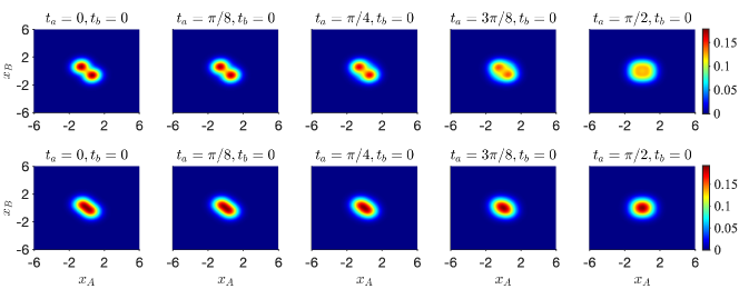
The above calculation assumes that the measurement at “collapses” the system at into one or other of the coherent states, or , at the time of the measurement, . The calculations based on that assumption can now be rigorously validated, since we give a specific proposal, that the measurement at site be performed as a quadrature phase amplitude measurement . The spin is the sign of the outcome . In this section, we carry out a complete analysis by evaluating as in Section III.C. The results shown in Figures 12 and 13 confirm the prediction of the violation of the Leggett-Garg-Bell inequality (28) and (4) for large .


The dynamics of the measurement and its disturbance is visualised, by plotting sequences of the function (Figure 14). In order to measure or , via the measurable moments and , one measures the spin at (top and centre sequences). In order to measure via the measurable moment , one measures the spin at time (with no measurement at ). The measurements are made by stopping the evolution at at the time , or , respectively.

The top two sequences of Figure 14 show measurement of or , where the system at is frozen at , so that information about the state of the system at time is stored at that site , and continues to evolve. We see from the plot of for and (last plot of the centre sequence) that . Similarly, the plot for and (last plot of the top sequence) shows . The lower sequence of Figure 14 corresponds to a measurement at site made at time , in order to evaluate . The evolution at ceases at so that the value for can be measured. The system continues to evolve, until . The correlations giving are indicated by the final plot of the lower sequence. We find and hence . The exact values for the correlations are evaluated numerically by integration of the joint distributions at the specified times. The calculation given in the Appendix leads to
| (37) | |||||
where is the error function. Results are shown in Figure 13, in agreement with the simple approach of the last section.
The pictures of Figure 11 are also justified for this measurement procedure. The impact of whether the measurement takes place at time , or not, is seen to be minimal if we examine the marginal (reduced) state for the system A, immediately after time . This is consistent with the idealised model of the measurement given in Figure 11. If there was no measurement at , and the measurement was made at time , then the system at time is in a superposition of the two coherent states. On the other hand, if a measurement is made at time , then the marginal (reduced) state for is the mixture, since no preparation took place at and the statistics for the system is given by (LABEL:eq:bellunitary). The marginal Q functions in each case are (48) and (LABEL:eq:q2-2), given as the second plots of the two sequences in Figure 11, which give indistinguishable predictions for large , justifying the arguments that this is an (apparently) non-disturbing measurement.
Despite the negligible difference in the marginal Q functions for system at the time , a macroscopic difference in the joint correlations measured between and emerges at the later time (and indeed, has already emerged at the time ). The correlations shown in Figures 12 and 14 imply results for the two-time moments corresponding exactly to those shown in the final plots of the two sequences of Figure 11. The macroscopic difference between the final plots of the two sequences in Figure 11 arises over the timescale of the unitary evolution that determines the measurement this is the evolution seen in the first three plots of the centre and lower sequence, of Figure 14. The subsequent dynamics at after leads to the macroscopic difference in correlations seen in the final plots of the sequences of Figure 11. On very short timescales (evident at of Figure 14) as the unitary rotation takes place, we note the system cannot be considered a two-state system.
V Delayed collapse
V.1 Delaying the collapse stage of the measurement
We now clarify a possible point of confusion about the timing of the final readout (the “collapse” stage) of the measurement at , for the Leggett-Garg-Bell proposal of Section IV.B. The measurement of is done by measuring at time and inferring from the correlation between the two systems, and . The measurement of comes in two stages: First, it is necessary to stop the unitary interaction of system at the time , so that information from the correlation can be stored. The second stage of the measurement at constitutes the irreversible “collapse”, where there is a coupling to a detector. While the timing of the first stage is crucial, the timing of the “collapse” stage at is immaterial.
To clarify, we compare where the collapse at has, or has not, occurred prior to the time of the (collapse) measurement of at . First, let us assume the collapse at has not occurred. Here, the two systems and are prepared in the entangled Bell state at time . System does not evolve further (), while system evolves for a time . The state formed after the evolution at is the superposition
| (38) |
The final joint distribution that describes the statistics at the later time , assuming there has been no prior collapse at , is calculated straightforwardly for this superposition state, as shown in the Appendix.

Now let us assume the final stage of the measurement at was made at the time , meaning that the pointer measurement consisting of a readout of the value of spin occurred at this time. In this case, the system has been coupled to a third system, so that a “collapse” occurs, for the system (and also for ). The system immediately after is given as the mixture (eqn (LABEL:eq:mixqstate)). The subsequent evolution is different to the evolution of the superposition (38). If a measurement is made at the later time , the joint probability is readily calculated, as shown in the Appendix. The two probabilities and are indeed different, due to the interference terms present for the superposition state, where the collapse does not occur. However, for and large, the two probabilities are indistinguishable.
The result is illustrated in Figure 15 where we consider measurements of and , for both small and large and . The Q functions depicted in the final plots of the top and lower sequences directly reflect the probabilities and for the two cases, where collapse has not, and has, taken place, respectively, by the time of the detection at . Although numerically different, these plots are, in effect, indistinguishable, for .
A similar result occurs if we consider the measurement of . It makes no effective difference to the joint probabilities whether or not the final collapse stage of the measurement at is delayed until a later time. The details are given in the Appendix.
V.2 Interpreting the delayed-collapse cat-state experiment
We ask what can be concluded from the Leggett-Garg-Bell experiments described in Sections IV and V.A, where the collapse stage of the measurement can be delayed? The latter will imply that one can perform the macroscopic Bell and Leggett-Garg tests as delayed choice and quantum eraser experiments delayed-choice-qubit . This follows naturally from the mapping from the microscopic to macroscopic qubits, which is ideal in the limit of large , for the angle choices needed for the delayed choice experiments. The new feature, compared to former delayed-choice experiments, is that the results are at the macroscopic level, where the qubit spin values reflect the macroscopically distinct amplitudes.
An argument can be given for interpretating the delayed collapse gedanken experiment in a way that is consistent with the premise of weak macroscopic realism (wMR). Here, the definition of wMR includes the assumption of macroscopic locality for the pointer (MLP) at A, as defined in Section III.E. The argument is based on the macroscopic nature of the experiment. After the time , the final collapse stage of the measurement at gives information about the macroscopic value of the spin of system (should it be measured). The delayed-collapse analysis of Sections V.A confirms that this information can be revealed at system an infinite time after , and after further events at . The system can be separated from by an infinite distance. A strong argument can then be given that carrying out the collapse stage of the measurement at does not macroscopically change the state-description of at the former time i.e. does not change the outcome for the macroscopic spin at .
We note that the wMR interpretation does not mean that prior to the measurement of spin at the system is in the quantum state or , since these states are microscopically specified, giving predictions for all measurements that might be performed on . That the system in the cat state cannot be viewed as a classical mixture can be negated in multiple ways, e.g. by observing fringes in the distribution for the orthogonal quadrature (for a single system ) or by deducing an Einstein-Podolsky-Rosen (EPR) paradox for the entangled state , along the lines given in Refs. eric_marg-1 ; irrealism-fringes ; macro-coherence-paradox ; macro-pointer ; Bohm-1 ; epr-1 ; bohm-eric ; epr-r2 . We give an example of this in the next subsection.
The consistency with wMR is explained as follows. Suppose the systems and are prepared at a time in a macroscopic superposition of states with definite outcomes for pointer measurements and , an example being (as )
| (39) |
Here, the states with definite outcomes for and are the states with definite outcomes for the spin . The assumption of wMR asserts that the system at the time is in one or other of two macroscopically specified states and , for which the result of a measurement of spin is deterministically predetermined i.e. the system at time may be described by a macroscopic hidden variable . For the bipartite system, wMR is to be consistent with MLP. MLP asserts that the value of the macroscopic hidden variable for the system cannot be changed by any spacelike separated event or measurement at the system that takes place at time e.g. it cannot be changed by a future event at . The interpretation is that the system at each time , and was in one or other of states or with a definite value of spin , and that the failure of macrorealism arises from the initial entanglement as the systems evolve dynamically at the intermediate times.
The assumption of MLP is to be distinguished from the stronger assumption, macroscopic locality (ML), introduced earlier, as part of the premise of macroscopic local realism (MLR). The premise of ML assumes locality to apply for spacelike separations where the measurement on system can vary, so that is not necessarily prepared in the pointer basis. The above wMR interpretation is thus not contradicted by the violation of macroscopic Bell inequalities. In fact, we have seen in Section III that, consistent with the validity of wMR, there is no violation of these Bell inequalities when there is no unitary transformation at . This is because in that case the system is in (immediately prior to the measurements) a state where wMR applies.
V.3 Einstein-Podolsky-Rosen-type paradox based on macroscopic realism
The EPR argument argues the incompleteness of quantum mechanics based on the assumption of local realism, or local causality epr-1 . One may also argue an EPR-type paradox for the cat states based on the validity of weak macroscopic realism. Here, we apply the argument given in Ref. macro-coherence-paradox .
One considers the superposition state (for large), similar to that prepared at the time in the Leggett-Garg-Bell tests. Here, . Macroscopic realism postulates that the system in such a state is actually in one or other state and for which the value of the macroscopic spin is predetermined. The spin is measured by the sign of : the distribution gives two separated Gaussian peaks, each with variance .
One may specify the degree of predetermination of for the macroscopic states, and , by postulating for each state and that the variance be some specified value, which we take as and respectively. If we assume each of and to be quantum states, then for each the Heisenberg uncertainty relation implies . We then argue, as was done in ref. macro-coherence-paradox , that for the ensemble of systems in a classical mixture of such states, and , we require , where , and . The observation of
| (40) |
implies incompatibility of macroscopic realism with the completeness of quantum mechanics, since the localised states and cannot be given as quantum states.
If we take , to match that the states have the variances associated with the two Gaussian peaks (the coherent states), we find the condition (40) is satisfied for . This is indeed the case for the superposition above. The distribution is
| (41) |
which shows fringes, as given in ref. yurke-stoler-1 . The variance is macro-pointer , indicating a paradox.
VI Conclusion
In this paper, we have provided ways to test quantum mechanics against macroscopic realism using cat states. We consider two definitions of macroscopic realism. The first, macrorealism (M-R), supplements the assumption of macroscopic realism with the premise of macroscopic noninvasive measurability. The second, macroscopic local realism (MLR), supplements with the premise of macroscopic locality. In this paper, “macroscopically distinct” refers to separations well beyond the quantum noise level .
In Sections II-IV, we show that quantum mechanics predicts failure of MLR (and M-R) for two spacelike-separated systems prepared in entangled cat states, in a way that is directly analogous to the original Bell and Leggett-Garg proposals. To test MLR, we consider CHSH-type Bell inequalities and three-time Leggett-Garg-Bell inequalities, where measurements are made at two spacelike separated locations, at successive times. One may construct similar tests, based on the Leggett-Garg-Bell inequality described in Section II, involving four times.
The tests give a convincing strategy to demonstrate the non-invasiveness of a measurement that is assumed in a Leggett-Garg test of macro-realism. For a macroscopic system, the usual argument is that the disturbance (at least for some ideal measurement) becomes vanishingly small, so as to have a negligible affect on the later dynamics. In order to refute the criticism that there is a disturbance, methods have been developed to quantify the effect of such a disturbance, if macroscopic realism is satisfied. One approach performs a control experiment that prepares two macroscopically distinguishable states ( and ) and then quantifies the effect of disturbance on the inequality, if the system is indeed in one of those states NSTmunro-1 . A counterargument however is that the system at time is in a state microscopically different to (or ), a state which was not prepared in the laboratory. In the present paper, such criticisms are avoided, because macroscopic realism is defined more broadly. One does not assume that the macroscopically distinct states are specific states and , nor that the states are quantum states. A direct disturbance due to measurement is ruled out, because the result for the measurement of is inferred from the measurement on the separated system . The non-classicality is then explained by quantum nonlocality, but at a macroscopic level.
In Section V, we have extended the bipartite Leggett-Garg analysis, to demonstrate that a delay of the final irreversible stage of the measurement makes no difference to the predictions, provided the amplitude of the coherent states is large. This implies that one could perform delayed choice experiments, similar to those examined for qubits in Refs. delayed-choice-qubit ; delayed-choice-interpretation . The possibility of delayed choice experiments is expected because of the mapping onto the qubit system, for large , (as the coherent states become orthogonal), for the rotation angles required for the qubit experiments. The new feature is the observation at a macroscopic level, since the qubits correspond to macroscopically distinct coherent states. As with the qubit experiments, this does not however imply acausal effects delayed-choice-interpretation .
It is clear from the violations of the macroscopic inequalities presented in this paper that MLR, macroscopic local causality (MLC), and M-R fail. We have explained in Section II that the MLR is defined as deterministic macroscopic (local) realism (dMR), that the system is predetermined to be in a state giving a definite outcome for the pointer measurement ( or ) prior to the unitary rotation that determines the measurement setting, or . The violation of the macroscopic Bell inequalities given in this paper show that dMR fails.
The results are however consistent with an interpretation in which a weak macroscopic realism (wMR) holds. The initial Bell state gives predictions for joint probabilities at time that are only microscopically different (of order ) to those of a non-entangled mixture. Yet, after the choice of measurement setting, the final joint probabilities are macroscopically different. In the wMR interpretation, the macroscopic differences arise during the unitary dynamics, corresponding in a Bell experiment to the choice of measurement setting. Such dynamics shifts the system into a superposition of states with definite outcomes for the measurement of the macroscopic spin , at a given time . The assumption of wMR postulates that a system in a superposition is describable by a macroscopic “element of reality”, , which predetermines the result of the pointer measurement for the macroscopic qubit value . The interpretation is that the system is in one or other states and giving a definite value for the macroscopic pointer measurement.
An EPR-type paradox arises from the assumption of weak macroscopic realism, if correct. The element of reality “state”, or , of the system prior to the measurement cannot be a quantum state. This is evident from calculations given in macro-coherence-paradox and explained in section V.C, where the states or that would apply to the cat state can be shown to be inconsistent with the uncertainty principle. Similar paradoxes have been illustrated for the two-slit experiment using the concept of irrealism irrealism-fringes , and for entangled cat states eric_marg-1 , based on the logic of the original EPR paradoxes that reveal the inconsistency of the completeness of quantum mechanics with local realism epr-1 ; Bohm-1 ; bohm-eric ; epr-r2 .
Finally, we comment on the possibility of an experiment. Entangled cat states have been generated cat-bell-wang-1 . The challenge is to realise the unitary rotation, given by the nonlinear Hamiltonian which has a quartic dependence on the field intensity. This is necessary for the full Bell experiment. However, a macroscopic delayed choice/ quantum eraser experiment may be carried out more straightforwardly, since this depends only on the creation of a simple cat state superposition, which can be realised at times from the nonlinear Kerr interaction yurke-stoler-1 ; manushan-cat-lg . This interaction has been experimentally achieved collapse-revival-bec-2 ; collapse-revival-super-circuit-1 .
Acknowledgements
This research has been supported by the Australian Research Council Discovery Project Grants schemes under Grant DP180102470.
Appendix
VI.1 Calculation of Bell violations
The joint probability is where , are eigenstates of and respectively. Using the overlap , we find
| (42) |
VI.2 Interference effects
Where , the joint probability for outcomes and for the system prepared in the entangled superposition (32) is
| (43) | |||||
This contains an interference term proportional to that vanishes with large . The expression reduces to the result for the mixture , given by
| (44) |
because the interference term contains the expression which is small for orthogonal state, with large .
By contrast, for and , we compare the expressions for the evolved cat state given by of eq. (LABEL:eq:234-1-1-1), with that of the evolved mixture
| (45) | |||||
The expressions are the same apart from interference terms, such as
| (46) |
We see from the solutions given by eqs. (LABEL:eq:state3-20) that for the suitable choices of , (for example) may involve terms such as , and involves terms in . This then leads to a contribution of type and therefore significant interference terms (when ). These terms are the origin of the macroscopic difference between the probability distributions in Figures 6 for nonzero and , which leads to the macroscopic Bell violation.
VI.3 Leggett-Garg test for a single system: Q function dynamics
The Q function at time is that of a coherent state where we take to be real.
| (47) |
At time , the system is in the superposition state (29) which has the Q function
| (48) |
where . Assuming no measurement takes place at time , the system at time is in the superposition state (30) with
| (49) |
If the measurement is performed at , the system “collapses” to either (with probability ) or (with probability ) and then evolves at time respectively to either or as given by eqn. (29).
There are two cases to compare: whether or not a measurement is performed at time . Figure 12 shows the sequence for the Q functions at the times , and for these two cases. The top sequence, modelling where a measurement is not performed, shows sequentially the three Q functions, (47), (48) and (49). The lower sequence plots where a measurement is performed at time , assuming this is done in such a way to instigate a collapse into one or other of the coherent states, as described above. The second plot of the lower sequence is therefore the Q function
representing the average state of the system at time , immediately after the measurement at time : . The Q function for the final state at time , if the measurement has taken place at time , is given by the evolution of for the time . The final average state is where . The Q function is
| (51) |
which is plotted as the third function of the lower sequence.
VI.4 Bipartite Leggett-Garg tests: correlation between the outcomes at the different sites
Here, we evaluate and the value of the conditional probabilities where for the case . These quantities are worked out exactly as one would measure them. We first evaluate at time .
| (52) |
where we use
| (53) |
In fact, because the system at time remains in a Bell state (apart from a phase factor), this also represents for the time . We note that
| (54) |
which on integration gives . For the value of the conditional probability , , one measures
| (55) |
Similarly, we evaluate
| (56) |
where . This gives the result (37). The plots of Figure 13 and 15 reveal that for , the positive and negative values for the outcomes of correspond to distinct macroscopically separated Gaussian peaks in the different quadrants. The conditional probability goes to as is larger, which justifies that the measurement of at indicates the value at .
VI.5 Delayed Collapse for measurement
The state formed after the evolution at is the superposition
| (57) |
The final joint distribution at time is (assuming there has been no prior collapse at )
| (58) | |||||
Now let us assume the final stage of the measurement at was made at the time , meaning that the pointer measurement consisting of a readout of the value of spin occurred at this time. In this case, the system has been coupled to a third system, so that a “collapse” occurs, for the system (and also for ). The system (or rather, an ensemble of them) immediately after is given as the mixture (eqn (LABEL:eq:mixqstate)). The system then evolves from a state that is either or , which is different to the evolution of the superposition (57). If a measurement is made at the later time , the joint probability is
| (59) | |||||
The two probabilities are indeed different. However, for and large, examination shows that the two probabilities (58) and (59) become indistinguishable.
VI.6 Delayed collapse for measurement
We may also examine where a measurement is to be made at time , as in the evaluation of . Again, it makes no difference as to the evaluation, if the “collapse” stage is delayed until a later time. Wishing to measure the spin of subsystem at time means we then “stop” the evolution of system at . If the system continues to evolve, then the state of the system is ()
| (60) |
The final distributions and are similar to those above, replacing by . The lower sequence of Figure 15 shows the Q function dynamics for the evolution where there has been no collapse at time . When plotted, the sequence where a collapse has occured shows, even for moderate , no distinguishable difference, in either the final measured probabilities or the Q function.
?refname?
- (1) J. S. Bell, Physics 1, 195 (1964).
- (2) J. F. Clauser, M. A. Horne, A. Shimony and R. A. Holt, Phys. Rev. Lett. 23, 880 (1969). J. S. Bell, Foundations of Quantum Mechanics ed B d’Espagnat (New York: Academic) pp171-81 (1971). J. F. Clauser and A. Shimony, Rep. Prog. Phys. 41, 1881 (1978).
- (3) N. Brunner, D. Cavalcanti, S. Pironio, V. Scarani, and S. Wehner, Rev. Mod. Phys. 86, 419 (2014).
- (4) H. M. Wiseman, Journ. Phys A 47, 424001 (2014).
- (5) N. D. Mermin, Phys. Rev. D 22, 356 (1980). P. D. Drummond, Phys. Rev. Lett. 50, 1407 (1983). J. C. Howell, A. Lamas-Linares, and D. Bouwmeester, Phys. Rev. Lett. 88, 030401 (2002). M. D. Reid and W. J. Munro, Phys. Rev. Lett. 69, 997 (1992). M. D. Reid, Phys. Rev. Lett. 84, 2765 (2000). H. Jeong, M. Paternostro and T. C. Ralph, Phys. Rev. Lett. 102, 060403 (2009). M. Navascués, D. Pérez-García and I. Villanueva, J. Phys. A: Math. Theor. 46 085304 (2013). J. Tura, R. Augusiak, A. B. Sainz, B. Lücke, C. Klempt, M. Lewenstein, A. Acínac, Annals of Physics 362, 370 (2015). B. J. Dalton, arXiv (2018), arXiv:1812.09651 [quant-ph]. A. B. Watts, N. Y. Halpern and A. Harrow, arXiv:1911.09122v1 [quant-ph].
- (6) N. D. Mermin, Phys. Rev. Lett. 65, 1838 (1990). A. Gilchrist, P. Deuar and M. D. Reid, Phys. Rev. A60, 4259 (1999). K. Wodkiewicz, New Journal of Physics 2, 21 (2000). G. Svetlichny, Phys. Rev. D 35, 3066 (1987). D. Collins et al., Phys. Rev. Lett. 88, 170405 (2002). J. Lavioe et al., New J. Phys 11, 073051 (2009). C. Wildfeuer, A. Lund and J. Dowling, Phys. Rev. A 76, 052101 (2007). F. Toppel, M. V. Chekhova, and G. Leuchs, arXiv:1607.01296 [quant-ph] (2016).
- (7) U. Leonhardt and J. Vaccaro, J. Mod. Opt. 42, 939 (1995). A. Gilchrist, P. Deuar and M. Reid, Phys. Rev. Lett. 80 3169 (1998). K. Banaszek and K. Wodkiewicz, Phys. Rev. Lett. 82 2009 (1999). Oliver Thearle et al., Phys. Rev. Lett. 120, 040406 (2018). A. Ketterer, A. Keller, T. Coudreau, and P. Milman, Phys. Rev. A 91, 012106 (2015).
- (8) A.S. Arora and A. Asadian, Phys. Rev. A 92, 062107 (2015). Ming-Da Huang, Ya-Fei Yu, and Zhi-Ming Zhang, Phys. Rev. A 102, 022229 (2020).
- (9) M. D. Reid, Phys. Rev. A 62, 022110 (2000). M. D. Reid, Phys. Rev. A 97, 042113 (2018).
- (10) M. Navascués and H. Wunderlich, Proc. Roy. Soc. Lond. A 466, 881 (2009).
- (11) A. Leggett and A. Garg, Phys. Rev. Lett. 54, 857 (1985).
- (12) E. Schroedinger, 23, 807 (1935). F. Frowis, P. Sekatski, W. Dur, N. Gisin, and N. Sangouard, Rev. Mod. Phys. 90, 025004 (2018).
- (13) A. N. Jordan, A. N. Korotkov, and M. Buttiker, Phys. Rev. Lett. 97, 026805 (2006).
- (14) N. S. Williams and A. N. Jordan, Phys. Rev. Lett. 100, 026804 (2008).
- (15) C. Emary, N. Lambert, and F. Nori, Rep. Prog. Phys 77, 016001 (2014). A. Palacios-Laloy, F. Mallet, F. Nguyen, P. Bertet, Denis Vion, Daniel Esteve and Alexander N. Korotkov, Nature Phys. 6, 442 (2010). M. E. Goggin, M. P. Almeida, M. Barbieri, B. P. Lanyon, J. L. O’Brien, A. G. White, and G. J. Pryde, Proc. Natl. Acad. Sci. 108, 1256 (2011). G. Waldherr, P. Neumann, S. F. Huelga, F. Jelezko, and J. Wrachtrup, Phys.Rev. Lett. 107, 090401 (2011). G. C. Knee et al., Nature Commun. 3, 606 (2012). Z. Q. Zhou, S. Huelga, C-F Li, and G-C Guo, Phys. Rev. Lett. 115, 113002 (2015). C. Robens, W. Alt, D. Meschede, C. Emary, and A. Alberti, Phys. Rev. X 5, 011003 (2015). J. A. Formaggio et al., Phys. Rev. Lett. 117, 050402 (2016).
- (16) J. Kofler and C. Brukner, Phys. Rev. A 87, 052115 (2013); L. Clemente and J. Kofler, Phys. Rev. Lett. 116, 150401 (2016).
- (17) G. C. Knee, K. Kakuyanagi, M.-C. Yeh, Y. Matsuzaki, H. Toida, H. Yamaguchi, S. Saito, A. J. Leggett and W. J. Munro, Nat. Commun. 7, 13253 (2016).
- (18) J. Dressel and A. N. Korotkov Phys. Rev. A 89, 012125 (2014). J. Dressel, C. J. Broadbent, J. C. Howell and A. N. Jordan, Phys. Rev. Lett. 106, 040402 (2011). T. C. White et al., NPJ Quantum Inf. 2, 15022 (2016). B. L. Higgins, M. S. Palsson, G. Y. Xiang, H. M. Wiseman, and G. J. Pryde, Phys. Rev. A 91, 012113 (2015).
- (19) A. Asadian, C. Brukner, and P. Rabl, Phys. Rev. Lett. 112, 190402 (2014). C. Budroni, G. Vitagliano, G. Colangelo, R. J. Sewell, O. Gühne, G. Tóth, and M. W. Mitchell, Phys. Rev. Lett. 115, 200403 (2015). J. J. Halliwell, Phys. Rev. A 93, 022123 (2016). L. Rosales-Zárate, B. Opanchuk, Q. Y. He, and M. D. Reid, Phys. Rev. A 97, 042114 (2018). L. Rosales-Zárate, B. Opanchuk, and M. D. Reid, Phys. Rev. A 97, 032123 (2018). A. K. Pan, Phys. Rev. A 102, 032206 (2020). J. Halliwell, A. Bhatnagar, E. Ireland, H. Nadeem and V. Wimalaweera, arXiv:2009.03856v3 [quant-ph]
- (20) M. Thenabadu and M. D. Reid, Phys. Rev. A 99, 032125 (2019).
- (21) R. Uola, G. Vitagliano and C. Budroni, Phys. Rev. A 100, 042117 (2019).
- (22) M. Thenabadu, G-L. Cheng, T. L. H. Pham, L. V. Drummond, L. Rosales-Zárate and M. D. Reid, Phys. Rev. A 102, 022202 (2020).
- (23) See M. D Reid and M. Thenabadu, accompanying letter.
- (24) D. Gočanin, A. Dimić, F. D. Santo and B. Dakić, Phys. Rev. A, 102, 020201(R) (2020).
- (25) A Peres, “Quantum Theory Concepts and Methods”, (Kluwer Academic Publishers) (1995).
- (26) J. Kofler and C. Brukner, Phys. Rev. Lett. 101, 090403 (2008).
- (27) D. Poulin, Physical Review A 71, 022102 (2005). J. Kofler and C. Brukner, Phys. Rev. Lett. 99, 180403 (2007). S. Raeisi, P. Sekatski, and C. Simon, Phys. Rev. Lett. 107, 250401 (2011). T. Wang, R. Ghobadi, S. Raeisi, and C. Simon, Phys. Rev. A 88, 062114 (2013). H. Jeong, Y. Lim, and M. S. Kim, Phys. Rev. Lett. 112, 010402 (2014). J. Park, S.-W. Ji, J. Lee, and H. Nha, Phys. Rev. A 89, 042102 (2014). C. Duarte, G. D. Carvalho, N. K. Bernardes, and F. de Melo, Phys. Rev. A 96, 032113 (2017). P. Silva Correia and F. de Melo, Phys. Rev. A 100, 022334 (2019). O. Kabernik, Phys. Rev. A 97, 052130 (2018). C. Duarte, arXiv preprint arXiv:1908.04432 (2019). I. Veeren and F. De Melo, Phys. Rev. A 102, 022205 (2020).
- (28) S. D. Bartlett, T. Rudolph and R. W. Spekkens,Phys. Rev. A 86, 012103 (2012). R. W. Spekkens, Phys. Rev. A 75, 032110 (2007). N. Harrigan and R. W. Spekkens, Found. Phys. 40, 125 (2010).
- (29) A. Budiyono and D. Rohrlich, Nature Communications 8, 1306 (2017). A. Budiyono, Phys. Rev. A 100, 032125 (2019). ibid, Phys. Rev. A 100, 062102 (2019).
- (30) M. D. Reid, J. Phys. A: Math. Theor. 50, 41LT01 (2017).
- (31) P. D. Drummond and M. D. Reid, Phys. Rev. Research 2, 033266 (2020).
- (32) M. J. Hall, D. Deckert and H. Wiseman, Phys. Rev. X 4, 041013 (2014).
- (33) Y. Aharonov, E. Cohen, F. Colombo, T. Landsberger, I. Sabadini, D. Struppa and J. Tollaksen, Proc. Nat. Acad. Sci. 114, 6480 (2017).
- (34) A. Einstein, B. Podolsky, and N. Rosen, Phys. Rev. 47, 777 (1935).
- (35) M. D. Reid, Phys. Rev. A 100, 052118 (2019).
- (36) F. R. Lustosa, P. R. Dieguez, and I. G. da Paz, Phys. Rev. A 102, 052205 (2020).
- (37) E. G. Cavalcanti and M. D. Reid, Phys. Rev. A. 77, 062108 (2008). L. Rosales-Zarate, R. Y. Teh, S. Kiesewetter, A. Brolis, K. Ng, and M. D. Reid, J. Opt. Soc. Am. B 32 A82 (2015). R. Y. Teh, L. Rosales-Zárate, B. Opanchuk, and M. D. Reid, Phys. Rev. A 94, 042119 (2016).
- (38) Kôdi Husimi (1940). Proc. Phys. Math. Soc. Jpn. 22: 264.
- (39) C. Wang et al., Science 352, 1087 (2016).
- (40) B. Yurke and D. Stoler, Phys. Rev. Lett. 57, 13 (1986).
- (41) E. Wright, D. Walls and J. Garrison, Phys. Rev. Lett. 77, 2158 (1996).
- (42) M. O. Scully and K. Drühl, Phys. Rev. A 25, 2208 (1982). S. P. Walborn, M. O. Terra Cunha, S. Pádua, and C. H. Monken, Phys. Rev. A 65, 033818 (2002). Y.-H. Kim, R. Yu, S. P. Kulik, Y. H. Shih and M. O. Scully, Phys. Rev. Lett. 84 (2000). A. Peruzzo, P. Shadbolt, N. Brunner, S. Popescu and J. L. O’Brien, Science 338 6107, (2012).
- (43) Xiao-Song Ma et al., Proceedings of the National Academy of Sciences. 110 (4) (2013); B. G. Englert, M. O. Scully, and H. Walther, Am. J. Phys. 67, 325 (1999). Sandro Faetti, arXiv:1912.04101 [quant-ph]. Xi. Ma, J. Kofler, and A. Zeilinger, Rev. Mod. Phys. 88, 015005 (2016).
- (44) D. Bohm, “Quantum Theory” (Constable, London 1951).
- (45) M. D. Reid, Phys. Rev. A 40, 913 (1989). M. D. Reid, P. D. Drummond, W. P. Bowen, E. G. Cavalcanti, P. K. Lam, H. A. Bachor, U. L. Andersen and G. Leuchs, Rev. Mod. Phys. 81, 1727 (2009).
- (46) E. G. Cavalcanti, P. D. Drummond, H. A. Bachor and M. D. Reid, Optics Express 17 (21), 18693 (2009).
- (47) M. Greiner, O. Mandel, T. Hånsch and I. Bloch, Nature 419, 51 (2002).
- (48) G. Kirchmair et al., Nature 495, 205 (2013).