Bi-center conditions and bifurcation of limit cycles in a class of -equivariant cubic switching systems with two nilpotent points
Abstract
In this paper, we generalize the Poincaré-Lyapunov method for systems with linear type centers to study nilpotent centers in switching polynomial systems and use it to investigate the bi-center problem of planar -equivariant cubic switching systems associated with two symmetric nilpotent singular points. With a properly designed perturbation, 6 explicit bi-center conditions for such polynomial systems are derived. Then, based on the center conditions, by using Bogdanov-Takens bifurcation theory with general perturbations, we prove that there exist at least small-amplitude limit cycles around the nilpotent bi-center for a class of -equivariant cubic switching systems. This is a new lower bound of cyclicity for such cubic polynomial systems, increased from to .
keywords:
Nilpotent singular point; -equivariant switching system; bi-center; focus; cusp; limit cycleMSC:
34C07, 34C231 Introduction
In recent years, there have been extensive studies on the qualitative behaviours of nonsmooth dynamical systems, associated with the vector fields which are either discontinuous or nondifferentiable. The main reason of the increasing interest in these studies is that many practical systems contain nonlinearity and nonsmoothness in their equations and display rich complex dynamical phenomena, as observed in biology [40], nonlinear oscillation [7, 29], dry friction of mechanical engineering [5, 30], power electronics [3] and so on. In fact, fundamental mathematical theory for such nonsmooth systems was established several decades ago, see [1, 41].
Switching system is one important class of nonsmooth systems, which is divided into several regions with different definitions of smooth vector fields. In this paper, we consider the switching systems described in the form of
| (1) |
where , are analytic functions, and the boundary between these two regions defines the switching manifold. Although the vector field could be neither continuous nor differentiable on the boundary , we recall the Filippov convention [18] that the vector field may be crossing, sliding on or escaping from the boundary. Before presenting our main results, we give an overview on two main problems in the qualitative theory of planar differential vector fields, namely, the center problem and the cyclicity problem.
We recall that an isolated singular point is monodromy in a planar vector field if all nearby orbits rotate about this point. It is well known [2] that a monodromic singular point can only be a center or a focus. The center problem is to determine whether a monodromic critical point is a center or a focus, see [20]. But this problem becomes extremely complicated in the switching systems described by (1). To overcome the difficulty, the authors of [21] presented a useful approach for computing the Lyapunov constants of switching systems, which can be used to derive the linear type center conditions for an elementary singular point characterized by a pair of purely imaginary eigenvalues. This type of centers can be determined by vanishing all the Lyapunov constants. In [9, 10, 24] a complete classification with conditions is given to determine if a singular point is a linear type center for several classes of switching systems. Nevertheless, for a given particular class of polynomial systems, finding a complete solution of the center problem is still extremely difficult.
For a given family of differential systems, the Lyapunov constants needed to solve the center problem are also related to the so called cyclicity problem, i.e., finding the maximum number of limit cycles around a singular point. The investigation on bifurcation of limit cycles in switching systems started a half century ago. In [26], Han and Zhang presented an interesting example to show that limit cycles can bifurcate in switching linear systems from a pseudo-focus, i.e., a focus of either focus-focus, parabolic-focus or parabolic-parabolic type, which cannot occur in smooth linear systems. Later, Freire et al. [19], Huan and Yang [28] independently proved that switching linear systems can have at least limit cycles. Bastos et al. [4] proved that the number of crossing limit cycles in switching linear systems is at least , which has two regions separated by a cubic curve. Tian and Yu [42] constructed a special class of switching Bautin systems to show the existence of limit cycles in the neighborhood of a center. Recently, by using the averaging method, Braun et al. [6] obtained a new lower bound with 12 limit cycles bifurcating in quadratic switching systems. On the other hand, by the so-called pseudo-Hopf bifurcation analysis, one more limit cycle can be generated by a proper perturbation. However, not many works have been focused on the studies of cubic switching systems. Yu et al. [46] proved that cubic switching systems can have at least 18 limit cycles around two elementary foci. Chen et al. [12] presented a method to study the cyclicity problem in the neighborhood of the origin and infinity for a class of cubic switching systems. The maximal number of limit cycles obtained so far for cubic switching systems by perturbing an elementary center is , see [23, 38].
The aim of this paper is to study the center and cyclicity problems associated with nilpotent singular points in switching systems. Let us recall some known results about nilpotent singular points. An isolated singular point of a planar polynomial system is said to be a nilpotent singular point if both eigenvalues of the Jacobian matrix of the system evaluated at this singular point are zero but the Jacobian matrix is not identically null. The authors of [14, 22, 31, 44, 39, 45] developed some computationally efficient methods for studying the nilpotent center problem of smooth systems. García [20] presented a technique for bounding the maximal number of limit cycles bifurcating from a family of nilpotent singular points in some symmetric smooth polynomial systems. Recently, Li et al. [32] obtained the conditions on two nilpotent singular points to be centers in a class of cubic smooth systems, and proved that limit cycles exist around each of the two nilpotent singular points, with more limit cycles bifurcating from two elementary second-order foci which are generated by breaking the first-order nilpotent foci, leading to a total of limit cycles, which is up to now the best result for cubic systems with nilpotent singular points.
However, the center problem and bifurcation of small-amplitude limit cycles for nilpotent singular points in switching systems become more challenging than that in the case of elementary centers. Facing the challenging, we generalize the Poincaré-Lyapunov method to compute what will be called generalized Lyapunov constants for switching nilpotent systems, and apply the method to study the bi-center problem and the cyclicity problem for a class of -equivariant cubic switching systems with two symmetric nilpotent singular points. Here, we say that a -equivariant differential system, whose global phase portraits are invariant under a rotation of () radians around the origin, has a bi-center at the singular points and if both the two singular points are centers, which will be called bi-center problem. The study of -equivariant polynomial systems is closely related to the well-known Hilbert’s 16th problem, for more details see [13, 33, 34, 36, 37].
Without loss of generality, the -equivariant cubic switching systems, based on (1) which satisfies (with the switching manifold defined as the -axis)
can be written in the form of the differential equations,
| (2) |
where the -axis is the switching manifold and all parameters are real. As is known, the type of nilpotent singular points can generate much more rich dynamics than that of the elementary one, such that the center of system (2) in the switching manifold can be made up of two center-focus (a center or a focus), or one cusp and one center-focus, or two cusps. In this paper, we assume that system (2) has two nilpotent singular points located at , and derive the conditions which ensure the nilpotent singular points of (2) to be bi-center for two cases of critical points, namely, the third-order critical point and the second-order critical point. Moreover, we apply general perturbations to prove the existence of at least small-amplitude limit cycles bifurcating from the nilpotent bi-center , two of them are obtained from a symmetric pseudo-Hopf bifurcation by adding a suitable additional perturbation term. This is a new lower bound (increased from to ) on the number of limit cycles bifurcating in such cubic switching systems associated with nilpotent singular points.
The rest of the paper is organized as follows. In Section 2, we will simplify system (2) for the convenience of analysis and present our main results. In Section 3, we present some formulas which are needed in Sections 4 and 5 for proving the two main theorems. Section 4 is devoted to derive conditions for of system (2) to be bi-center. Then, in Section 5 we use the center conditions to construct perturbed systems of (2) to show the bifurcation of limit cycles from the nilpotent singular points . Finally, conclusion with discussion on future work is given in Section 6.
2 Simplification of system (2) and the main results
Assuming that system (2) has two singular points at yields that
| (3) |
The Jacobian matrices of (2) evaluated at are given by
| (4) |
It follows from that
| (5) |
To have being isolated nilpotent singular points, the necessary and sufficient conditions are , but is not identically zero. It is easy to obtain that , and (but not ), which gives either or , that is
| (6) |
However, when and , system (2) becomes
| (7) |
It is easy to note that the polynomial equations in (7) have a common factor , and so are not isolated singular points. Thus, .
Further, to make be isolated nilpotent singular points of system (2), we set
| (8) |
which leads to . With the above results, system (7) is reduced to
| (9) |
For the sake of convenience, we call the system in (9) for “the upper system” and that for “the lower system”.
Now, we need to discuss the multiplicity of the nilpotent singular points for the upper and the lower systems in (9). In fact, by the symmetry of system (9), we only need to analyze the singular point . Introducing the transformation into system (9) results in
| (10) |
and thus the singular point of system (9) is shifted to the origin of system (10). Assume that
are the unique solutions of the implicit function equations . Further, we denote that
| (11) | ||||
where
| (12) | ||||
For planar smooth systems, if is the smallest integer satisfying , then the multiplicity of the nilpotent singular point is exactly , for more details see [32]. Thus, we can use Theorem 3.5 in [16] to determine the type of the nilpotent singular point of (10) for the smooth polynomial equations either in the upper system or in the lower system.
More precisely, when and , we have that
| (13) |
When , and , we have that
| (14) |
where H-E denotes the local phase portrait with one singular point consisting of one hyperbolic sector and one elliptic sector.
Proposition 2.1.
The multiplicity of the nilpotent singular point of the upper system or of the lower system of (9) is at most 6.
Proof.
Using (12) with , we have
First, assume that . Then, we obtain . If , we have , and so is not an isolated singular point, implying that . If , we have . Letting yields , and then and have a common factor . Hence, if is an isolated singular point.
Next, assume that . Then, we have . Setting
we have and
If , we have . Further, we obtain that and have a common factor , leading to . Otherwise, we assume that , under which . Then, we have
If , we obtain that and have a common factor . If , we have . Then and have a common factor . Hence, is not an isolated singular point, implying that . ∎
Next, we derive the conditions for the nilpotent singular points (,0) of the -equivariant cubic switching system (9) to be bi-center, yielding the following result.
Theorem 2.2.
The nilpotent singular points (,0) of system (9) become bi-center if one of the following conditions holds:
| (15) | ||||
Moreover, to find the maximal number of limit cycles around the nilpotent singular points (,0) of system (9), we construct perturbed -equivariant switching systems using the bi-center conditions and prove that system (9) has at least limit cycles bifurcating from the nilpotent singular points (,0). More precisely, we have the following theorem.
Theorem 2.3.
Under each of the nilpotent bi-center conditions in Theorem 2.2, the -equivariant cubic switching system (9) has at least limit cycles bifurcating from the two symmetric nilpotent singular points by using all -order cubic perturbation, and at least limit cycles by, in addition, applying a symmetric pseudo-Hopf bifurcation.
3 The generalized Poincaré-Lyapunov method
In this section, for the convenience of reading, we first briefly describe the Poincaré-Lyapunov method for determining the linear type center in switching polynomial systems divided by the -axis, and then generate this method to study switching systems associated with isolated nilpotent singular points. As described in [10], we consider the following switching system,
| (16) |
where , . Let represent two parameter vectors. The origin is a common singular point in both upper and lower systems of (16). With the polar coordinate transformation: and , system (16) can be rewritten as
| (17) |
where and are polynomials in the parameters and . We suppose that the solutions for the upper and the lower systems of (17) are respectively obtained as and satisfying the initial condition . Then, we denote by
and
the upper half-return map and the lower half-return map , respectively, where ’s are the coefficients in Taylor expansions. Following the procedure in [21], we obtain the displacement function,
| (18) |
where is called the th-order Lyapunov constant of system (16). The origin of system (16) is a center if and only if all the Lyapunov constants in (18) vanish, i.e., for . If there exists such that and , then any perturbations to system (16) can yield at most limit cycles bifurcating from the origin. Based on Lemma 4 in [42], we give the sufficient conditions for proving the existence of limit cycles bifurcating from the origin of system (16).
Lemma 3.1 ([42]).
If there exists a critical point such that , , with , and
| (19) |
then appropriate small perturbations about lead to that system (16) has exactly limit cycles bifurcating from the origin.
It is worth mentioning that a switching polynomial system can have one more small-amplitude limit cycle when the sliding segment changes its stability by adding constant terms, which is called pesudo-Hopf bifurcation, see [15, 18]. With and , we assume that and are given in (16), but has the following form
| (20) |
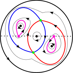
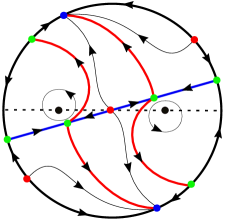
Then, the upper system of (16) still has a singular point at the origin, while the lower system of (16) has a singular point near the origin. System (16) would have a sliding segment on the switching manifold (the -axis). For small enough , the new switching system exhibits a pseudo-Hopf bifurcation at , as shown in Figure 1, which can produce one more small-amplitude limit cycle, see more details in [8].
In the above discussions, we have briefly described the Poincaré-Lyapunov method and the pesudo-Hopf bifurcation for switching polynomial systems with linear type centers. Now, we consider the switching polynomial system with a nilpotent critical point at the origin,
| (21) |
where and are real analytic functions without constant and linear terms. We will show that the Poincaré-Lyapunov method can be generalized to analyze center problem and bifurcation of limit cycles for the nilpotent singular point.
We give the following example to illustrate our idea, as the normal form of the nilpotent differential system can be simplified into the system (for example, see [25]),
| (22) | ||||
where , , and are analytic functions satisfying . For the sake of simplicity, we consider a codimension-2 Bogdanov-Takens (B-T) bifurcation of the cubic normal form (22). Then, we obtain the following normal form with unfolding:
| (23) | ||||
where the term is called unfolding with sufficiently small parameters and . Note that the origin of system (23) is a linear type singular point when and . When , , the linear type origin becomes a nilpotent singular point.
We remark that the linear type origin of system (23) is a center if and only if , and that the nilpotent monodromic origin (when ) of system (23) is also a center when . Hence, the main idea of our method is to perturb system (21) and to establish a relation between the unperturbed system and the perturbed system based on the B-T bifurcation theory, which will generate perturbed Lyapunov constants.
To achieve this, we consider the following perturbed system of (21),
| (24) |
where is called unfolding with sufficiently small , and are real polynomials.
It should be noted that the -perturbation terms in (24) are applied to the whole system, not restricted to the local behavior. We use the rather than in the linear perturbation term to avoid the () and terms generalted in the later transformed systems. Based on B-T bifurcation theory and the relation established above for the two systems (21) and (24), we know that a nilpotent center can be -approximated by a linear type center. More detailed discussions on this subject can be found in [11].
For this type system of (24), we can apply the Poincaré-Lyapunov method and compute the generalized Lyapunov constants . As a matter of fact, we have the displacement function of system (24), given by
| (25) |
in which denotes the th -order Lyapunov constant. We can determine the center conditions for system (24) by vanishing the terms in these generalized Lyapunov constants, thus leading to a set of algebraic conditions which characterize the existence of a nilpotent center of system (21).
Further, we can use the above generalized Poincaré-Lyapunov method to study the bifurcation of limit cycles from the nilpotent center of the switching system (21). By B-T bifurcation theory, we add a linear perturbation term to system (21) such that the origin of this switching system becomes a linear-type center. Then, we compute the generalized Lyapunov constants of the perturbed system with additional all -order perturbation terms. Following the procedure in [17], we can obtain the bifurcation of limit cycles from the nilpotent center as many as possible. Finally, we obtain one more limit cycle in the switching system by considering the pseudo-Hopf bifurcation.
4 The proof of Theorem 2.2
Since the multiplicity of monodromic critical point for smooth nilpotent systems is (see [16]), we know that the smallest multiplicity for a singular point is if it is a nilpotent focus or center. For the sake of convenience, we call the singular point with multiplicity the 3rd-order critical point. However, the multiplicity of the monodromic singular point in switching systems can be , i.e., a 2nd-order critical point. Hence, we consider four cases in the following two subsections.
4.1 The rd-order critical point of the upper system in (9)
By using the conditions given in (13) and (14), we obtain that the singular point of the upper system of (9) is a 3rd-order nilpotent focus or center if and only if
| (26) |
namely,
| (27) |
Then, we obtain
When , i.e., , the singular point of the lower system in (9) is a cusp. On the other hand, the singular point of the lower system in (9) is a center or a focus with multiplicity if (i.e., ), and . In order to have a monodromic singular point at of (9), it requires that there do not exist seperatrices which connect this singular point in the upper system or the lower system. With the aid of Maple, we present the following example to demonstrate a phase portrait of system (9), indicating that the lower system of (9) has two seperatrices connecting in the lower half Poincaré disc when . Thus, we only need to consider .
Example 4.1.
To discuss the bi-center conditions for of system (9), we assume that , as given in (27). Then, we show how to apply the Poincaré-Lyapunov method to derive the bi-center conditions for of system (9). By the symmetry of system (9), we only need to study the center conditions at the singular point .
With the transformation applied and perturbations added to system (9) with (27), we obtain the following perturbed system, can check from (10)
| (28) |
where
in which , are real parameters.
Note that system (28) should be invariant under the transformation (since and are symmetric singular points of (9)), which yields
| (29) |
where represent or .
Since system (28) has a large number of perturbation parameters, which makes the calculation of the generalized Lyapuov constants very difficult, we need to reduce the number of parameters. Without loss generality, we assume that because they are redundant for proving the necessity of the conditions I-VI. Further, we consider only the -order perturbed terms, i.e., setting (). The reason for why only choosing -order perturbed terms will be given in Section 5.
For convenience, we let . Further, introducing the transformation into system (28), we obtain
| (30) |
To give a clear view of the proof, we first present a table below to show the flow of the proof.
| Cases | Conditions | ||||
| (i) | I | ||||
| (ii) | (ii-1) | II | |||
| (ii-2) | II | ||||
| (ii-3) | (ii-3-1) | (ii-3-1-1) | (ii-3-1-1-1) | II, III | |
| (ii-3-1-1-2) | — | ||||
| (ii-3-1-2) | (ii-3-1-2-1) | II | |||
| (ii-3-1-2-2) | II | ||||
| (ii-3-1-2-3) | — | ||||
| (ii-3-1-2-4) | II, IV | ||||
| (ii-3-2) , , | (ii-3-2-1) | — | |||
| (ii-3-2-2) | — | ||||
The basic idea of the proof is setting the generalized Lyapunov constants zero to get a number of “necessary” center conditions, and excluding those which make certain order Lyapunov constant non-zero, and then later we prove that the remaining necessary conditions are also sufficient.
With the aid of a computer algebra system, we use the Poincaré-Lyapunov method to compute the generalized Lyapunov constants associated with the origin of system (30). The first two generalized Lyapunov constants are , and
Setting the -order and -order terms in zero yield the necessary center conditions,
Then, the rd generalized Lyapunov constant is given by
From the previous analysis for the multiplicity, we only consider two cases (i) and (ii) .
-
(i)
Assume that . Letting the -order, -order and -order terms in equal zero we obtain the conditions,
Then, we have the 4th generalized Lyapunov constant, given by
Thus, we obtain the conditions by setting the -order and -order terms in zero. Therefore, the necessary center conditions are , giving the condition I.
-
(ii)
Assume that . By setting the -order and -order terms in zero we obtain the conditions,
Then, we obtain the th generalized Lyapunov constant,
We have the following three subcases (ii-1) , (ii-2) and (ii-3) . Note that in the following analysis, when the condition in one case is satisfied, the conditions in other two cases may hold or not hold, depending upon the analysis for each case. In subcase (ii-3-1-1), both conditions and are satisfied.
(ii-1) Assume that . Then, we have by setting , yielding the condition II.
(ii-2) Assume that . Since the parameter is redundant for the analysis of this subcase, without loss of generality, we let . If , we have by using , which gives a special case of the condition II. Otherwise, if , we have by setting -order term of zero. Then, the 5th generalized Lyapunov constant becomes
Setting the -order term in zero we obtain . Further, letting we have
Letting the -order term in zero we obtain . Then, the 6th generalized Lyapunov constant becomes
where
By computing the resultant of and with respect to we have
which implies that and have no common roots. Hence, we obtain from . Then, we obtain the 7th generalized Lyapunov constant,
which indicates that the -order term in is non-zero when .
(ii-3) Assume that . Then, we have and obtain the 5th generalized Lyapunov constant,
where
Two subcases follow : (ii-3-1) and (ii-3-2)
(ii-3-1) When we have . In order to have that the -order term in equals zero, it needs or .
(ii-3-1-1) Assume that , we have . Then, we obtain the simplified ,
(ii-3-1-1-1) If
from we have , which gives a special case of the condition II, or
which does not contain the perturbed parameters, as expected, giving the condition III. Further there exists the free parameter such that .
(ii-3-1-1-2) If
we have
from . Letting
from , which yields . Then, from the -order term of ,
which also giving the special case of the condition II and the condition III. In fact, from the -order term and -order term of , we have the resultants of , , and with respect to , respectively,
i.e., there exist the free parameters such . Then we have .
We remark that since the parameter is redundant for the following subcases, without loss of generality, we let .
(ii-3-1-2) Assume that . We solve the polynomial equations: to find other real solutions for parameters , , and .
(ii-3-1-2-1) If , we have , and either or by using the equations . The first solution is included in the condition II. For the second solution, if we obtain and the 7th generalized Lyapunov constant, given by
Setting yields , leading to and
Hence, we obtain that the -order term in is not vanished.
(ii-3-1-2-2) If , by setting we obtain , which is included in the condition II.
(ii-3-1-2-3) If , we obtain
by solving . Further, we have and
But if , then .
(ii-3-1-2-4) Assume that . If , we have from , which is a special case of the condition II. Suppose that . Then, by using , we have that
where
Then, the polynomial becomes
where
To have , it requires under which , and the 7th generalized Lyapunov constant becomes
where
and
Since , we have . Then, to solve , we only need to find the solutions to the equations: . Thus, we compute the resultants of , , , and with respect to , respectively, and obtain
where , , are real constants, and
To find the common factors of the above resultants, we only need to consider the following three subcases due to .
(ii-3-1-2-4-1) If , we obtain the simplified polynomials,
If , we have , which yields violating the condition . If , we obtain from , which contradicts the condition .
(ii-3-1-2-4-2) Assume that . Similar to the above process, we use the equation with the constraint to obtain one set of parameter values:
Eliminating the perturbed parameter we obtain the condition IV.
(ii-3-1-2-4-3) Now assume and . We solve the equations: to obtain the solutions under which and the th generalized Lyapunov constant is simplified to
where , and are polynomials in , , and , with , and terms, respectively. We compute the resultants of , , and with respect to , respectively, and obtain
where , , are real constants, and , and are polynomials in , and , having 45 terms, 81 terms and 47 terms, respectively.
We again calculate the resultants of , , , with respect to , respectively, to have
where , , are real constants, and
while the polynomials , , do not have common nonzero roots. So, we only have possible solutions from . If , we solve to obtain , which yields , contradicting the condition . If , we solve to have , and either or , which violates .
Now, assume that . We have , and obtain the -order term in the th generalized Lyapunov constant, which is a polynomial in , and having terms. We compute the resultant of and with respect to to obtain
where is a real constant, and is a polynomial in and having terms. We again calculate the resultant of and with respect to , and have
where is a real constant, and is a th-degree polynomial in and . Since the resultant of and with respect to equals , where is a real constant, we conclude that there do not exist parameter values such that all -order terms in , and vanish.
(ii-3-2) Since we assume that and based on . If , we have , which is included in the condition II. Hence, we assume that . Similar to the analysis for the case (ii-3-1), we consider the two subcases and .
(ii-3-2-1) Under the condition , we assume that , which yields . Then, setting the -order term in zero we obtain , under which the polynomials and are simplified to
It is easy to find from that
Further, we have the following simplified polynomials:
Then, we compute the resultant of and with respect to to obtain
under the conditions: and . This shows that there are no parameter values satisfying .
(ii-3-2-2) Assume . Letting the -order term in be zero we have , yielding the following simplified polynomials:
Setting gives
We use the above solutions to simplify and to obtain the following polynomials:
By computing the Groebner basis for , , , , and , we obtain two polynomial equations:
which yields
under which , and the th generalized Lyapunov constant is simplified as
where , , are integers. Hence, any -order term in is non-zero under the condition and .
We have shown that the four conditions I, II, III and IV in Theorem 2.2 are necessary for the singular points of system (9) to be nilpotent bi-center. Now, we prove that these four conditions are also sufficient.
If the condition I in Theorem 2.2 holds, system (9) is reduced to
| (31) |
via . The upper and the lower systems in (31) are Hamiltonian systems, having respectively the Hamiltonian functions,
| (32) | ||||
which shows that the condition, , in Proposition 2.1 of [10] is satisfied, and so the origin of system (31) is a center. Hence, system (9) has a nilpotent bi-center at (,0), which consists of a monodromic singular point and a cusp.
If the condition II in Theorem 2.2 holds, the system (9) is simplified into a smooth one,
| (33) |
which is symmetric with respect to the -axis, so we know that the singular points (,0) of system (9) are bi-center.
If the condition III in Theorem 2.2 holds, system (9) again becomes a smooth one:
| (34) |
which has the algebraic integral curve,
giving an inverse integrating factor for this system. Thus, system (9) has a nilpotent bi-center at (,0).
If the condition IV in Theorem 2.2 holds, system (9) is a smooth one:
| (35) |
Actually, for an arbitrary nonzero constant , by the transformation,
system (35) can be changed to
| (36) |
which implies that system (35) is invariant under the following transformation . Hence, we can always choose proper to satisfy , yielding . Then, the origin of system (35) is a center according to the condition of Theorem 4.2 in [32].
4.2 The nd-order critical point of the upper system in (9)
In this subsection, we consider the center conditions associated with of the first system of (9) with multiplicity two. Thus, assume that , i.e., . Then, the singular point in the upper smooth system of (9) is a cusp. If , then in the lower system of (9) is a 3rd-order critical point. If , in the lower smooth system of (9) is also a cusp. Similarly, recall that the singular point () cannot be a monodromic singular point when , and hence we only consider the case when . Therefore, combining and we have either or .
Example 4.3.
We apply the generalized Poincaré-Lyapunov method again to system (9) with either or . Introducing the transformation into system (9), we obtain the perturbed system,
| (37) |
which satisfies the condition (29) for the perturbed parameters.
Similarly, we first present a table to outline the proof for the center conditions V and VI.
| Cases | Conditions | |||
| (i) | (i-1) | (i-1-1) | (i-1-1-1) | V |
| (i-1-1-2) | V | |||
| (i-1-2) | (i-1-2-1) | V | ||
| (i-1-2-2) | — | |||
| (i-2) | (i-2-1) | VI | ||
| (i-2-2) | VI | |||
| (ii) | VI | |||
The first two generalized Lyapunov constants at the origin of system (37) are
Setting we get the necessary center condition: , , for system (37). Then, it follows from the discussion given at the beginning of this subsection that we consider two cases: (i) and (ii) .
-
(i)
By the -order term of , we have two subcases (i-1) and (i-2) .
(i-1) If , we have . Then, the rd generalized Lyapunov constant is given by
By setting the -order term in zero we have the following two subcases: (i-1-1) and (i-1-2) .
(i-1-1) Assume that . Letting the -order and -order terms in zero we obtain
Then, we have the th generalized Lyapunov constant,
Two subcases follow the -order term in to be zero: (i-1-1-1) , and (i-1-1-2) .
(i-1-1-1) If , we obtain by , giving the condition V.
(i-1-1-2) If , we obtain and
from . Further, we have
where
It follows from that , which is included in the condition V. Otherwise, the -order term in is non-zero.
(i-1-2) Assume and . Letting the -order and -order terms in zero, we obtain
Then, we have the th generalized Lyapunov constant,
Letting the -order terms in zero we have .
(i-1-2-1) If , the -order term in becomes zero. By using we have . Then, the th generalized Lyapunov constant is simplified as
If , we obtain the condition included in the condition V. Otherwise, the -order term in does not equal zero.
(i-1-2-2) If , the -order term in again becomes zero. From we obtain . Then, we have the th generalized Lyapunov constant,
where
If we have . Hence, by using we have , and
Setting the -order term in zero we have . Further, we have the simplified Lyapunov constant,
which has a non-zero -order term.
(i-2) If , we obtain the rd generalized Lyapunov constant,
Similar to the previous case, we have the following two subcases: (i-2-1) and (i-2-2) .
(i-2-1) If , setting the -order, -order and -order terms in to equal zero yields
Further, we have
By using we have and , giving the first condition in VI.
(i-2-2) If , vanishing each order term in yields
Then, we obtain the th generalized Lyapunov constant,
It follows from that , and , which also leads to the first condition in VI.
-
(ii)
If , similar to the analysis for the subcase (i-2), replacing by in , then we obtain the second condition in VI.
The above discussions (or see Table 2) show that the conditions V and VI are necessary for the origin of the perturbed system (37) to be a center, and so they are necessary conditions for (,0) of the unperturbed system (9) to be nilpotent centers. We can also prove that these conditions are sufficient.
If the condition V in (15) holds, system (9) is reduced to
| (38) |
It is easy to see that system (38) is symmetric with respect to the -axis, and so by the symmetry of switching systems redefined in Theorem 2.1 of [35], it implies that the singular points (,0) of the system (9) are bi-center, which consists of two 2nd-order nilpotent cusps.
If the condition VI in (15) holds, via , system (9) becomes
| (39) |
Then it can be shown that the upper and lower systems in (39) are Hamiltonian systems, having respectively the Hamiltonian functions:
| (40) | ||||
It is straightforward to verify that the condition in Proposition 2.1 of [10] is satisfied, indicating that the origin of system (39) is a center. Hence, system (9) has bi-center at (,0).
Example 4.4.
The proof for Theorem 2.2 is completed.
5 The proof of Theorem 2.3
In this section, we will perturb system (9) with the center conditions in (15) to find the maximal number of small-amplitude limit cycles bifurcating from the bi-center. Since system (9) is symmetric with the origin, we only need to study the limit cycles around the singular point . Using each of the center conditions, we can show that system (9) can have small-amplitude limit cycles around each of the bi-center, and then plus additional small limit cycle from the pseudo-Hopf bifurcation, leading to a total of small-amplitude limit cycles bifurcating from the bi-center. Perturbations up to cubic terms are applied to system (9), and it will be shown that there exist maximal (including both system parameters and perturbation parameters) independent perturbation parameters. Therefore, small-amplitude limit cycles may bifurcate from each of the bi-center. Since the proofs for the center conditions I-VI are similar, we only prove one case for the center condition VI. It has been noted that for the first center conditions I-V, when the conditions are obtained to satisfy , then and equal zero simultaneously under a same condition, for which , implying that maximal small-amplitude limit cycles many exist around each of the bi-center. For the th center condition VI, solutions exist such that , , again indicating the existence of maximal small-amplitude limit cycles.
In order to include all possible perturbations, we add the perturbations including all () order terms to system (9) under the center condition VI to obtain
| (41) |
where
| (42) | ||||
With the transformation , the first two polynomials in (42) become
| (43) | ||||
In order to keep the origin of the corresponding shifted system to be a monodromic point, we eliminate the constants and the and terms in each -order term of and , and obtain
Similarly, simplifying in (42) yields
Next, with a simple parametrization: and , we have the following four translational perturbations:
| (44) | ||||
Therefore, under the transformation , system (41) becomes the following perturbed system,
| (45) |
By the approach described in [43] we introduce the following near-identity state transformation and time rescaling:
| (46) |
for the upper system in (45), where
| (47) |
A similar transformation can be used to simplify the lower system in (45). Note that the unperturbed system of (45) is unchanged by the identity map (46). Therefore, we may obtain proper ’s to simplify the perturbations without loss of generality. By substituting (46) into system (45) and taking the -order terms, we obtain
| (48) |
and
| (49) |
Now, simplify setting
eliminates the terms , , in the equation, and the terms , in the equation. It implies that the perturbations
| (50) |
in (45) are redundant and can be removed. Thus, we assume that . Further, introducing the transformation, into system (45) yields
| (51) |
To further simplify system (51), we apply the following scaling,
| (52) |
to (51), and obtain
| (53) |
Therefore, the singular point of system (9) corresponds to the origin of system (53). To compute the generalized Lyapunov constants (), we let , which yields . It is seen from (53) that there exists an infinite number of parameters, but most of them are redundant. Without loss of generality, we let
| (54) |
which, together with , are substituted into (53) to yield the final system,
| (55) |
for computing the generalized Lyapunov constants . Returning to system (51), (55) becomes
| (56) |
We will show that system (56) can have at least small-amplitude limit cycles around the origin.
Now, system (55) has only independent parameters: , , , , , , and , which will be used to solve the Lyapunov equations . Note that later we will perturb the constant term to obtain one more limit cycle by using the pseudo-Hopf bifurcation. The 1st generalized Lyapunov constant for system (55) is given by when . Then, we have the 2nd generalized Lyapunov constant,
Setting yields and the 3rd generalized Lyapunov constant,
We obtain
by solving . Further, we have the 4th generalized Lyapunov constant,
Since the condition required for the center condition VI does not allow , we have . Thus, solving for we obtain
Then, solving the 5th generalized Lyapunov constant equation for yields
leading to
where , , , , and are polynomials in , , and . In particular,
and other lengthy expressions of , , , and are omitted for brevity. Here, we assume that
| (57) |
Then, we use Maple with its built-in command eliminate,
to obtain a solution , where
and
and three polynomial resultant equations,
Further, we apply the command eliminate again to the three resultants to obtain a solution , and two lengthy polynomial resultants,
where , , and are lengthy polynomials in and , with , , and terms, respectively. There are four combinations: , , and to find the solutions for . However, it can be shown that only the combination generates maximal number of limit cycles. Finally, we use the Maple-built command resultant,
to obtain the following resultant,
| (58) | ||||
where is a big positive integer, and are respectively th-degree and th-degree polynomials in . With the aid of Maple using digits accuracy, we obtain , and real solutions from the terms in the script bracket of , the polynomials and , respectively.
Remark 5.1.
In most research articles, researchers prefer to not use numerical computation in a rigorous mathematical proof. Here, we should point out that (1) our numerical computation is only used at the last step, and all computations in the previous steps are symbolic and exact. (2) we can, instead of using numerical computation, apply the interval computation (or interval arithmetic) [27] to prove the existence of the solutions in an interval satisfying a required accuracy. This does not really change the basics of computation, and a numerical computation makes the presentation simple and clear. (3) the most important point is that the accuracy to be taken (e.g., decimal points) should be good enough to guarantee the reliability of proof. That is, the accumulation of round errors in the numerical computation does not affect the conclusion for the existence of solutions. In other words, it is not a matter of numerical computation, but the high enough accuracy.
It can be shown that all the solutions obtained from produces , but , giving small amplitude limit cycles. While from the solutions, we obtain solutions (with ):
which result in , but . Moreover, all the solutions satisfy the requirement of the center condition VI,
We choose one of the solutions,
where the subscript C indicates a critical point, under which
More precisely, with the accuracy of decimal points, we have
for which we are definitely confident that a solution exists, satisfying . In addition, a direct calculation shows that
Hence, by Lemma 3.1 we know that system (53) has at least small-amplitude limit cycles bifurcating from the origin, leading to the existence of small-amplitude limit cycles bifurcating from the bi-center of such -equivariant cubic switching systems.
Further, applying the pseudo-Hopf bifurcation, we obtain one more small-amplitude limit cycle for system (56) by perturbing the coefficient . For and sufficiently small, the switching system (56) has a small sliding segment on the switching manifold with the end points at and , where is the root of the equation in (56), namely,
which yields the solution . Thus, the sliding segment shrinks to when goes to zero.
We consider the point on the switching line with sufficiently small , where is defined as a bifurcation function, satisfying
| (59) |
Then, we have two half-return maps given in the form of
| (60) |
respectively, where
| (61) |
It follows from (59) and (60) that and , implying that when . Then, to get more small-amplitude limit cycles, we let , and compute higher-order generalized Lyapunov constants. This means that we return to exactly where we start and obtain the system (55) under the assumption . Therefore, by Lemma 3.1 and combining the small-amplitude limit cycles obtained above, we know that small-amplitude crossing limit cycles exist near the origin of system (56), and so small-amplitude limit cycles can bifurcate from the bi-center of the -equivariant cubic switching system (9).
Note that since we include all -order perturbations in constructing system (41), the number is actually the maximal number of small-amplitude limit cycles which can be obtained with the center conditions I-VI under Hopf and pseudo-Hopf bifurcations for the -equivariant cubic switching system considered in this paper.
This finishes the proof for Theorem 2.3.
6 Conclusion
In this paper, we have studied the bi-center problem and the cyclicity problem for planar switching nilpotent systems. First, we generalize the Poincaré-Lyapunov method for switching systems with linear-type centers to compute the generalized Lyapunov constants for switching nilpotent systems. Then, we derive bi-center conditions for cubic -equivariant switching systems with two symmetric nilpotent singular points. In particular, we find that the bi-center consists of the combination of two second-order nilpotent cusps. Further, we construct perturbed systems with the center conditions and present one with the center condition VI to show the existence at least small-amplitude limit cycles bifurcating from the nilpotent bi-center, which provides a great improvement from , leading to a new lower bound on the number of limit cycles in -equivariant cubic switching systems.
Motivated from this work, some questions naturally arise, which may promote future research in this direction.
-
1.
In this work, we use some special perturbation to obtain center conditions for -equivariant cubic switching system with nilpotent singular points. Does this special perturbation generate all possible center conditions? If not, what center conditions might be missed, and what kind of perturbations should be used to find all possible center conditions?
-
2.
The computation of the Lyapunov constants heavily depends upon a computer algebra system and the algorithms to be used. From this work, we have found that the current techniques for symbolic computation is good enough for computing the generalized Lyapunov constants. However, the current well-known approaches such as Groebner basis, regular chains, and Maple built-in programs eliminate, resultant, etc. seem still not powerful enough to solve the Lyapunov constant (polynomial) equations as well as many other such equations related to Hilbert’s 16th problem. So, how to develop a more efficient method (or algorithm, or program) for solving the system of multivariate polynomial equations is a very challenging task and needs further research.
-
3.
In this paper, our generalized Lyapunov constants contain different order terms (before scaling), and we treat them in a consistent way by scaling. However, in the literature, many works treat such Lyapunov constants or focus values according to the orders, similar to the consideration of the 1st-order, 2nd-order, etc. Melnikov functions (for example, see [43]). Then, what are the advantages and disadvantages of these two perturbation methods, and for what systems one of the two approaches is better to be applied?
Acknowledgment
This work was supported by the National Natural Science Foundation of China Nos. 12071091 (T. Chen), 12071198 (F. Li) and 12371175 (Y. Tian), the Guangdong Basic and Applied Basic Research Foundation No. 2022A1515011827 (T. Chen), the Project funded by China Postdoctoral Science Foundation No. 2023M744329 (T. Chen) and the Natural Sciences and Engineering Research Council of Canada, No. R2686A02 (P. Yu).
References
- [1] A. Andronov, A. Vitt, S. Khaikin, Theory of Oscillations, Pergamon Press, Oxford, 1966.
- [2] A. Algaba, C. García, J. Giné, J. Llibre, The center problem for -symmetric nilpotent vector fields, J. Math. Anal. Appl. 466 (2018) 183–198.
- [3] S. Banerjee, G. Verghese, Nonlinear Phenomena in Power Electronics: Attractors, Bifurcations, Chaos, and Nonlinear Control, Wiley-IEEE Press, New York, 2001.
- [4] J. Bastos, C. Buzzi, J. Llibre, D. Novaes, Melnikov analysis in nonsmooth differential systems with nonlinear switching manifold, J. Differential Equations 267 (2019) 3748–3767.
- [5] M.D. Bernardo, P. Kowalczyk, A.B. Nordmark, Sliding bifurcations: a novel mechanism for the sudden onset of chaos in dry friction oscillators, Int. J. Bifurcation Chaos 13 (2003) 2935–2948.
- [6] F. Braun, L. P. C. da Cruz, J. Torregrosa, On the number of limit cycles in piecewise planar quadratic differential systemss, (2023) preprint.
- [7] A. Buic, J. Llibre, O. Makarenkov, Asymptotic stability of periodic solutions for nonsmooth differential equations with application to the nonsmooth van der Pol oscillator, SIAM J. Math. Anal. 40 (2009) 2478–2495.
- [8] J. Castillo, J. Llibre, F. Verduzco, The pseudo-Hopf bifurcation for planar discontinuous piecewise linear differential systems, Nonlinear Dynam. 90 (2017) 1829–1840.
- [9] X. Chen, Z. Du, Limit cycles bifurcate from centers of discontinuous quadratic systems, Comput. Math. Appl. 59 (2010) 3836–3848.
- [10] X. Chen, W. Zhang, Isochronicity of centers in switching Bautin system, J. Differential Equations 252 (2012) 2877–2899.
- [11] T. Chen, L. Huang, P. Yu, Center condition and bifurcation of limit cycles for quadratic switching systems with a nilpotent equilibrium point, J. Differential Equations 303 (2021) 326–368.
- [12] T. Chen, L. Huang, P. Yu, W. Huang, Bifurcation of limit cycles at infinity in piecewise polynomial systems, Nonlinear Anal.: Real World Appl. 41 (2018) 82–106.
- [13] T. Chen, S. Li, J. Llibre, -equivariant linear type bi-center cubic polynomial Hamiltonian vector fields, J. Differential Equations 269 (2020) 832–861.
- [14] I. Colak, J. Llibre and C. Valls, Hamiltonian nilpotent centers of linear plus cubic homogeneous polynomial vector fields, Adv. Math. 259 (2014) 655–687.
- [15] L. Cruz, D. Novaes, J. Torregrosa, New lower bound for the Hilbert number in piecewise quadratic differential systems, J. Differential Equations 266 (2019) 4170–4203.
- [16] F. Dumortier, J. Llibre, J. Artés, Qualitative Theory of Planar Differential Systems, Universitext, Springer-Verlag, New York, 2006.
- [17] R.D. Euzébio, J. Llibre, D.J. Tonon, Lower bounds for the number of limit cycles in a generalised Rayleigh-Liénard oscillator, Nonlinearity 35 (2022) 3883–3906.
- [18] A.F. Filippov, Differential Equation with Discontinuous Right-Hand Sides, Kluwer Academic, Netherlands, 1988.
- [19] E. Freire, E. Ponce, F. Torres, A general mechanism to generate three limit cycles in planar Filippov systems with two zones, Nonlinear Dynam. 78 (2014) 251–263.
- [20] I. García, Cyclicity of some symmetric nilpotent centers, J. Differential Equations 260 (2016) 5356–5377.
- [21] A. Gasull, J. Torregrosa, Center-focus problem for discontinuous planar differential equations, Int. J. Bifurcation Chaos 13 (2003) 1755–1765.
- [22] H. Giacomini, J. Giné, J. Llibre, The problem of distinguishing between a center and a focus for nilpotent and degenerate analytic systems, J. Differential Equations 227 (2006) 406–426.
- [23] L. Gouveia, J. Torregrosa, Local cyclicity in low degree planar piecewise polynomial vector fields, Nonlinear Anal.: Real World Appl. 60 (2021) 103278 1-19.
- [24] L. Guo, P. Yu, Y. Chen, Bifurcation analysis on a class of -equivariant cubic switching systems showing eighteen limit cycles, J. Differential Equations 266 (2019) 1221–1244.
- [25] M. Han, P. Yu, Normal Forms, Melnikov Functions and Bifurcations of Limit Cycles, Springer-Verlag, New York, 2012.
- [26] M. Han, W. Zhang, On Hopf bifurcation in non-smooth planar system, J. Differential Equations 248 (2010) 2399–2416.
- [27] T. Hickey, Q. Ju, M. H. Van Emden, Interval arithmetic: From principles to implementation, J. ACM 48 (2001) 1038–1068.
- [28] S. Huan, X. Yang, Existence of limit cycles in general planar piecewise linear systems of saddle-saddle dynamics, Nonlinear Anal. 92 (2013) 82–85.
- [29] M. Kunze, T. Kupper, Qualitative bifurcation analysis of a non-smooth friction oscillator model, Math. Phys. 48 (1997) 87–101.
- [30] R. Leine, H. Nijmeijer, Dynamics and Bifurcations of Non-Smooth Mechanical Systems, Lect. Notes Appl. Comput. Mech., vol.18, Springer-Verlag, Berlin, 2004.
- [31] F. Li, H. Li, Y. Liu, New double bifurcation of nilpotent focus, Int. J. Bifurcation Chaos 31 (2021) 2150053.
- [32] F. Li, Y. Liu, Y. Liu, P. Yu, Bi-center problem and bifurcation of limit cycles from nilpotent singular points in -equivariant cubic vector fields, J. Differential Equations 265 (2018) 4965–4992.
- [33] F. Li, Y. Liu, P. Yu, J. Wang, Complex integrability and linearizability of cubic -equivariant systems with two 1:q resonant singular points, J. Differential Equations 300 (2021) 786–813.
- [34] F. Li, Y. Jin, Y. Tian, P. Yu, Integrability and linearizability of cubic systems with non-resonant singular points, J. Differential Equations 269 (2020) 9026–9049.
- [35] F. Li, P. Yu, Y. Tian, Y. Liu, Center and isochronous center conditions for switching systems associated with elementary singular points, Commun. Nonlinear Sci. Numer. Simul. 28 (2015) 81–97.
- [36] J. Li, Hilbert’s 16th problem and bifurcations of planar polynomial vector fields, Int. J. Bifurcation Chaos 3 (2013) 47–106.
- [37] J. Li, Y. Liu, New results on the study of -equivariant planar polynomial vector fields, Qual. Theo. Dyna. Syst. 9 (2010) 167–219.
- [38] J. Li, Y. Tian, Y. Liu, Twenty-six crossing limit cycles around one singular point in a cubic switching system, Int. J. Bifurcation Chaos 32(10) (2022) 2250158 (7 pages).
- [39] Y. Liu, F. Li, Double bifurcation of nilpotent focus, Int. J. Bifurcation Chaos 25(3) (2015) 1550036 (10 pages).
- [40] Y. Lv, R. Yuan, Y. Pei, Dynamics in two nonsmooth predator-prey models with threshold harvesting, Nonlinear Dynam. 74 (2013) 107–132.
- [41] N. Minorsky, Nonlinear Oscillations, Van Nostrand, New York, 1962.
- [42] Y. Tian, P. Yu, Center conditions in a switching Bautin system, J. Differential Equations 259 (2015) 1203–1226.
- [43] Y. Tian, P. Yu, Bifurcation of small limit cycles in cubic integrable systems using higher-order analysis, J. Differential Equations 264(9) (2018) 5950–5976.
- [44] E. Stróżzyna, H. Żoła̧dek, The analytic normal for the nilpotent singularity, J. Differential Equations 179 (2012) 479–537.
- [45] J. Yang, L. Zhao, The cyclicity of period annuli for a class of cubic Hamiltonian systems with nilpotent singular points, J. Differential Equations 263(9) (2017) 5554–5581.
- [46] P. Yu, M. Han, X. Zhang, Eighteen limit cycles around two symmetric foci in a cubic planar switching polynomial system, J. Differential Equations 275(2) (2021) 939–959.