![[Uncaptioned image]](https://cdn.awesomepapers.org/papers/9fab8c84-fa4b-4e73-bf8a-bf9e22413939/teaser_nice.png)
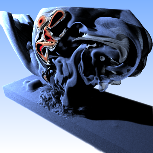
AMR rendering comparison using ExaBrick [WZU∗21] vs. our extended framework. Top-left: original “sci-vis style” rendering (old) with ray marching, local shading with on-the-fly gradients, and a delta light source. Bottom-right: volumetric path tracing (new) with multi scattering, isotropic phase function and ambient lighting. The original software used two RTX 8000 GPUs to render a convergence frame with all quality settings set to maximum at 4 frames/sec.; our framework, with the best combination of optimizations discussed in this paper, renders path-traced convergence frames with global illumination and significantly better image quality at 16 frames/sec. on a single GeForce RTX 4090 GPU.
Beyond ExaBricks: GPU Volume Path Tracing of AMR Data
Abstract
Adaptive Mesh Refinement (AMR) is becoming a prevalent data representation for HPC, and thus also for scientific visualization. AMR data is usually cell centric (which imposes numerous challenges), complex, and generally hard to render. Recent work on GPU-accelerated AMR rendering has made much progress towards real-time volume and isosurface rendering of such data, but so far this work has focused exclusively on ray marching, with simple lighting models and without scattering events or global illumination. True high-quality rendering requires a modified approach that is able to trace arbitrary incoherent paths; but this may not be a perfect fit for the types of data structures recently developed for ray marching. In this paper, we describe a novel approach to high-quality path tracing of complex AMR data, with a specific focus on analyzing and comparing different data structures and algorithms to achieve this goal.
1 Introduction
Adaptive Mesh Refinement (AMR) data is currently emerging as one of the most prevalent and important types of data that any visualization-focused renderer needs to be able to handle. Unfortunately, from a rendering point of view AMR data comes with several challenges: first, AMR data can come in many forms, from octree-AMR [BWG11] to various forms of block-structured AMR [CGL∗00]. Second, for rendering AMR data one requires a sample reconstruction method to be defined over the AMR cells’ scalar values; and how this is defined can have a huge influence on the images that the renderer produces. Third, most AMR data is highly non-uniform in nature, requiring the renderer to be able to concentrate its sampling effort where it matters most. Fourth, rendering AMR data is expensive partly because of the aforementioned issue of non-uniformity of the signal, and partly because of the hierarchical nature of the data. This means that each sample typically requires some form of hierarchical data structure traversal. Fifth, the recent advances in real-time ray- and path-tracing have raised the stakes for sci-vis rendering, too. While arguably, effects such as indirect illumination or soft shadows and ambient lighting are most important for photorealism, demand for high-quality Monte Carlo rendering is gradually becoming the de facto for sci-vis rendering as well. Particularly, this change in paradigm has been initiated by industry-quality tools like OSPRay [WJA∗17] or OpenVKL [KJM21], which are readily available to sci-vis users through ParaView or VisIt plugins [WUP∗18].
We explore the problem of high-quality path traced rendering of non-trivial AMR data sets (cf. Beyond ExaBricks: GPU Volume Path Tracing of AMR Data). For that we start with the ExaBrick AMR rendering framework by Wald et al. [WZU∗21], and look at what is required to extend this to volumetric path tracing. ExaBrick is both a framework and an acceleration data structure, similar to what kd-trees and BVHs are for surface ray tracing, and while fundamentally, there is no reason this acceleration data structure should not work with volumetric path tracing, it was not originally optimized for that. It is an open research question if this data structure optimized for sci-vis style volume ray marching can be easily adapted to support the fundamentally different operation of computing transmittance estimates as performed by a volumetric path tracer.
In contrast to ray marching, the dominating operation in volume path tracing is computing free flight distances, which require an upper bound estimate for the extinction of the volume density, called majorant. Though the method is correct irrespective of how much that upper bound over-shoots the real value, too high a difference between conservative majorant and actual extinction that varies in space causes unnecessary samples to be taken, so that key to accelerating volume path tracing is finding majorants that vary in space themselves and then form an acceleration structure.
In sci-vis, however–and in particular, for the type of data we are looking at in this paper–computing good majorants is hard: one factor is that actual extinction at any point in space depends on a transfer function that can map any data value to any extinction value, and which can—and typically will—undergo radical changes as the user explores the volume. A second factor is that the original AMR structure wants to adapt to the data, so that even if we were hypothetically allowed to relax the real-time requirement, finding good alpha-mapped majorants is a hard problem in itself.
Building upon these challenges in AMR visualization, the key contributions of this paper are the following:
-
•
We extend the AMR framework ExaBrick by replacing alpha-composited ray marching with volumetric path tracing, giving rise to significantly improved time to image for sci-vis rendering, plus the possibility to interactively create images with much better visual fidelity by using full global illumination.
-
•
We investigate the question how efficient the existing ExaBrick data structure is by systematically identifying and implementing all of the most obvious alternative variations of that approach.
-
•
We thoroughly analyze and compare the different alternatives and discuss their technical implications. This includes a comparison to a hypothetical (and due to its construction times impractical) reference data structure that is allowed to perform near unlimited preprocessing.
2 Related Work
Volume rendering is important for both scientific visualization (sci-vis) and production rendering, but opposing goals regarding visual fidelity on the one hand, and interactivity on the other hand, have led the two fields to take largely orthogonal approaches. Even early production rendering systems used scattering and virtual point lights [LSK∗07] and have since transitioned to full global illumination with multi scattering and hundreds of bounces [FHP∗18]. Scientific visualization has traditionally focused on interactive exploration [HKRs∗06] based on ray marching [Lev88] with absorption and emission [Max95]. Rendering with this lighting model can still be found in common scientific visualization systems like VisIt [CBW∗12] or ParaView [AGL05].
Exposure renderer [KPB12] is one of the first examples to use volumetric path tracing for sci-vis. It supports multi-scattering and can produce highly realistic images [MB17, IZM17]. However, volumetric path tracing only started to gain more attention from the community recently when optimized software and hardware ray tracing frameworks became widely available [WJA∗17, IGMM22]. Sci-vis renderers use simple isotropic phase functions covering the whole medium, RGB albedo from color lookup tables as opposed to full spectral rendering, and simple lighting models. Common techniques to compute free-flight distance estimates—the stochastic distance a photon travels without colliding with a particle from the density—are unbiased, which is attractive also for scientific visualization [MSG∗23].
A number of techniques exist to compute free flight distances and transmittance estimates using stochastic sampling. Woodcock (or delta-) tracking [WMPT65] is one of the oldest methods and virtually “homogenizes” the volume by introducing fictitious particles that produce null collisions where the ray is extended without a change in direction. Other estimators include decomposition tracking [KHLN17], residual ratio tracking [NSJ14], or unbiased ray marching using power series expansion [KDPN21].
Combined with spatially varying local majorants [NSJ14], unbiased transmittance and radiance estimates can be found much faster than with quadrature techniques, which is attractive for interactive exploration. In this sense, local majorants allow for the equivalent of empty space skipping and adaptive sampling, which are popular acceleration techniques in scientific volume rendering [ZSL19, ZSL21, WZM21]. In contrast to approaches that approximate the local frequency using the number of local cells and their sizes [MUWP19], majorants directly consider the actual frequency of the, which is represented by the local extinction.
Commonly used data structures that allow for traversal with local majorants are kd-trees [YIC∗10] as well as uniform macrocell grids that are traversed using the 3D digital differential analyzer (DDA) algorithm [SKTM11]. Bounding volume hierarchies (BVH) have received less attention as direct volume rendering accelerators, as the predominant techniques in sci-vis traditionally required ordered traversal. Morrical et al. [MSG∗23] used BVHs to accelerate an interactive volume path tracer, but concluded that a simple DDA grid implementation was more efficient. Approaches using BVHs as empty space skipping accelerators for volume rendering with front-to-back alpha compositing required the bounding boxes at the leaf nodes to not overlap [ZHL19]. The OpenVDB data structure that is popular in production rendering uses a hierarchical grid and DDA traversal with a fixed hierarchy size [Mus13]. Hofmann et al. [HE21] also provide a recent summarization of multi-level DDA traversal for volumetric path tracing on GPUs.
The term adaptive mesh refinement (AMR) was originally coined by Berger and Collela [BO84, BC89] at NASA. It refers to simulation codes that hierarchically subdivide a (often uniform) grid, both in space and in time, in regions where the simulation domain is more interesting than in others. Subdivision schemes include octrees [BWG11], or block-structured AMR [CGL∗00] where the rectangular regions are allowed to be irregular.
Virtually all existing AMR simulation codes (e.g., FLASH [DFG∗08], Lava [KBH∗14], etc.) output data that is cell-centric and results in T-junctions at odd level boundaries. Work by Wald et al. [WBUK17] and by Wang et al. [WWW∗19] has proposed interpolators that are continuous even at level boundaries, which is important for artifact-free visualization. These interpolators use sampling routines that perform neighbor queries by traversing tree data structures. If not carefully designed they require traversing those data structures per sample taken, resulting in non-trivial reconstruction costs infeasible for GPUs. ExaBrick by Wald et al. [WZU∗21], which is explained in more detail in Section 3.2, provides an acceleration structure to accomplish fast AMR cell location on GPUs.
For rendering octree-based AMR specifically, Wang et al. [WMU∗20] developed high-quality reconstruction filters for direct ray tracing. Other authors have also focused on large-scale out-of-core AMR rendering, such as the interactive streaming and caching framework proposed by Wu et al. [WDM22] targeted at CPU rendering, or the framework by Zellmann et al. [ZWS∗22], who proposed a similar method for AMR streaming and rendering on GPUs, but focused on time-varying data.
GPU path tracing native AMR data, to our knowledge, has not been proposed by the literature yet. Closest to this are OpenVKL [KJM21] that can path trace on the CPU but does not use any of the optimizations necessary for GPUs, and the framework proposed by Zellmann et al. [ZWMW23] that renders the AMR data by converting it to an unstructured mesh with voxels.
3 Background and Method Overview
In this section we discuss how to integrate volumetric path tracing (VPT) into a framework like Wald et al.’s ExaBrick [WZU∗21], which can render AMR data natively. A key requirement of our method is that VPT is compatible with RGB transfer functions that contribute albedo and extinction coefficients.
3.1 Scientific Visualization and Volumetric Path Tracing
In scientific visualization (sci-vis), volume renderers traditionally use the absorption plus emission model [Max95], often implemented with ray marching [Lev88], where for each screen space sample the volume is sampled at positions with uniform step size . At each position an indirect RGB transfer function lookup provides color and opacity. Final colors for the screen space sample are obtained via alpha compositing [PD84].
Rendering with volumetric path tracing (VPT) is fundamentally different in that opacity sampling and compositing are replaced with stochastically sampling the transmittance of light along a ray segment. The light then possibly (but not necessarily) bounces. Final screen space samples are averaged in the accumulation buffer instead of using alpha compositing. Despite (or probably even because of) those differences, the approach has merits also for sci-vis where it so far has not gained much attention yet.
The most notable advantage is that transmittance estimates are computed with much fewer volume samples than with ray marching. This comes at the cost of Monte Carlo noise, which however tends to converge over a few samples. Where the fast transmittance estimates pay off particularly is shadow computation: with a ray marcher, marching another volume ray towards the light source at each sample position is infeasible. With VPT a shadow ray is traced only when a collision occurs. This happens when (stochastically) the light is fully extinct and the free flight distance reached. Another advantage is that VPT is unbiased, which can give better correctness guarantees. Finally, it is perfectly viable to implement the absorption plus emission model based on the transmittance estimate routine used in VPT, and by that improving the time to (first) image, yet at the cost of introducing some noise.
We add VPT to the ExaBrick framework [WZU∗21]. A key change necessary is replacing the ray marcher used by ExaBrick with a tracking estimator that computes stochastic free fight distances that light passes through the volume without being blocked. Considering the Woodcock (also delta-) tracking algorithm [WMPT65] (cf. Algorithm 1) as an example, this estimator employs two stochastic processes–rejection and inversion sampling; rejection sampling depends on the so called majorant extinction coefficient for a region of space (in the following called , or if multiple majorants are encountered along a ray segment).
In Algorithm 1 a ray, given by its origin , direction , and range , is traversed through the volume. Rejection sampling decides if a null collision occurred; in that case, if the ray is still inside the tested segment, traversal continues in the same direction and another sample must be taken. This decision is made in line of Algorithm 1. The closer the majorant matches the actual density at the sample position , the less often the do…while loop is executed, and the less often the volume is sampled.
This gives rise to acceleration data structures over regions of space—or groups of objects—to find majorants that tightly bound the local density. This is indicated in Algorithm 1 by the outer for loop over all segments that the range is divided into; in practice, those segments are provided by a spatial accelerator like a grid or kd-tree, or by a bounding volume hierarchy (BVH). Below we explain in more detail how to implement such acceleration structures.
A requirement of sci-vis is that the volumes are color-mapped using RGB transfer functions; then becomes the extinction coefficient from Algorithm 1. RGB is interpreted as albedo, which gets evaluated during shading. Since now depends on the alpha transfer function, indirectly, so do the majorants . When spatially varying majorants are used as an acceleration data structure, hence, it is required that majorants can be recomputed interactively when the RGB map changes. However, naïvely iterating over every cell of the volume to recompute the majorants is infeasible for typical sci-vis data set sizes.
Instead, we pre-process the data storing, the min/max ranges with the accelerator leaves, as suggested by Knoll et al. [KWPH06]. When the RGB map changes, this allows us to iterate over the accelerator leaf nodes and use the min/max ranges as indices into the RGB map. The majorant for the accelerator leaf is the maximum value the RGB map takes on inside that range. In this paper, we assume that majorants are computed indirectly to maintain interactivity when updating transfer functions, but also seek to answer the question how much worse this is compared to a hypothetical pre-classified data structure without this restriction.
3.2 Extending the ExaBrick Framework
The ExaBrick framework and data structure have been explained in detail by prior works [WZU∗21, ZSM∗22, ZWS∗22]. We refer the reader to these for details. ExaBrick is a native AMR data structure, i.e., it does not resample or transform the AMR subgrids to unstructured elements, but samples the given cells directly. In its original form, ExaBrick was optimized to perform ray marching on GPUs. We extend this data structure to support volumetric path tracing. To our knowledge, volumetric path tracing using a native AMR sampling structure has not yet been proposed by the literature.
ExaBrick first generates bricks of same-level cells in the spirit of Kähler et al. [KSH03] so the builtin ray marcher can traverse relatively large coherent regions of space without requiring hierarchy traversals. Those bricks are much bigger in size than the original octree leaf nodes or block-structured AMR subgrids.
At the level boundaries, the bricks overlap by half a cell, to support reconstruction with tent-shaped basis functions. In the resulting overlap regions, filtered data values are obtained as a linear combination of the overlapping cell values. To make the non-convex overlap regions more rendering-friendly, Wald et al. subdivide them using a kd-tree. The domain boxes of the kd-tree leaves form what the authors call the active brick regions (ABRs).
An OptiX BVH is used to traverse the ABRs in hardware. Empty ABRs are culled when the alpha transfer function changes; adaptive sampling is achieved by adjusting the marcher’s step size to the size of the finest cell covered by the ABR. We extend the data structure to support VPT. For that we need to be able to support ray segment traversal as in Algorithm 1, to obtain local majorants that tightly bound the density along those segments, and support for point location queries to compute the local density and extinction coefficients using an AMR reconstruction filter.
The differences between a volume ray marcher and volumetric path tracer, and the challenges regarding memory access patterns are illustrated in Fig. 2. In the paper we explore different acceleration structures, including directly using the ABRs for segment traversal and sample reconstruction, but also evaluate alternative strategies. As in surface ray tracing, the quality of the acceleration structure has a large influence on performance, and it is unclear if the ABRs serve that purpose well. An example visualization of majorants obtained from ABRs is shown in Fig. 1.
We use CUDA and OptiX 7 to implement our extensions as this is the software framework also used by ExaBrick. We try to make use of hardware ray tracing where possible to accelerate segment traversal and sampling the AMR data structure.


4 Sci-Vis Volumetric Path Tracer
We implement volumetric path tracing (VPT) with OptiX 7. We support three visualization modes with different quality settings: absorption plus emission, realized with Woodcock tracking; single scattering, where an additional bounce to a light source chosen at random is performed to compute volumetric shadows; and multi scattering using a global phase function that allows the light to bounce arbitrarily. The different quality settings can have a tremendous impact on visual fidelity, as can be seen in Fig. 3.
Inside the OptiX ray generation program, we generate cameras ray with random jitter to compute screen space samples. For the tracking estimator implementation, the rays traverse an acceleration structure (as previously described); at each sampling position they compute the extinction coefficient by first sampling into the volume (using an AMR sample acceleration structure), and then post-classifying the sample using the RGB transfer function.
Given those two operations, which are described and evaluated in detail below—segment traversal and volume sampling—free flight distances are computed that are required by all three visualization modes. For the absorption and emission model, the sample color is proportional to the albedo from the transfer function at the position where the collision occurred. The single scattering estimator casts a shadow feeler towards a randomly chose light source, and the albedo gets weighted by the transmission between sample position and light source that we compute using ratio tracking [NSJ14]. In the case of multi scattering we evaluate a Henyey Greenstein phase function and perform bounces in a while loop inside the ray generation program. Based on the throughput, we terminate paths at random using Russian roulette.
Since we interpret the RGB component of the RGB transfer function as albedo, the path throughput is an RGB tuple as well—and so is the final screen space sample. We accumulate the screen space samples in a device-side accumulation buffer using a weighted average. Using an interactive prototypical viewer, whenever the camera changes, we reset accumulation. The accumulation buffer content is periodically presented as sRGB color tone mapped and drawn into an OpenGL pixelbuffer object mapped using CUDA/GL interop.
We describe how to implement the two core routines for VPT—ray segment traversal and AMR data sampling—in the following sections. The most obvious way to implement those operations is by using the existing ABRs (cf. Section 3.2). In the following sections, we explain the computation of ABR majorants and introduce alternative methods for spatial and object subdivision, which facilitate traversal and sampling of the AMR data structure.
5 Acceleration Structures for Traversal and Sampling
Volume acceleration data structures partition the ray into segments that each have their own majorant . Inside the segments, the rays are sampled. In this section we describe different strategies to implement those two operations. A restriction of hardware ray tracing is that when a ray traverses a BVH and the intersection or hit program is called, tracing rays against another hardware BVH is not permitted. It is thus not valid to use one BVH to traverse segments, and while integrating a segment traversing another BVH for sample reconstruction.
Alternatives to using two different hardware accelerated BVHs are using software acceleration structures for either of the operations; using the same acceleration structure for traversal and sampling; or halting the (outer) ray segment traversal for traversal, and then restarting it by setting the ray’s parameter to the previous segment’s . Each strategy we propose implements one of those alternatives.
5.1 Ray Segment Traversal Data Structures
In this subsection we discuss acceleration structures for ray segment traversal. Sampling data structures are discussed in Section 5.2. To facilitate interactive transfer function updates, all traversal accelerators (except the non-interactive reference described in Section 5.1.4) maintain two lists for each leaf node or leaf cell: one list with min/max ranges representing the actual data, and a list of majorants that is updated when the transfer function changes, by iterating over the list of ranges. The non-interactive reference stores the list of majorants only and does not support interactive transfer function updates.
5.1.1 Active Brick Region Traversal
One way to extend ExaBrick to obtain local majorants is to use the ABRs directly. The ABR extents are precomputed when the data set is loaded, and so is the list of min/max value ranges. One advantage of this mode is that it utilizes the same acceleration structure for both segment provisioning () and sampling, as the ABRs also store the overlapping brick IDs and with that all the information necessary for sample reconstruction (cf. Section 5.2.1); additional BVH traversal is hence not required.
5.1.2 Direct Brick Traversal
Another data structure that is directly available to us (although we usually do not maintain a traversal data structure for that) are the (Exa-)bricks themselves. While the default mode traverses ABRs, and bricks are only indirectly accessed during ABR traversal, it is also possible to traverse the bricks directly using an OptiX BVH.
We show min/max data range computation for bricks in Fig. 5. Every cell that overlaps a brick’s domain contributes its data value to the min/max range of that brick. We observe that the subdivision with bricks is much coarser than the ABR subdivision (cf. Fig. 4), so that a single overlapping cell can easily “infect” the whole brick with its value. A brick that would otherwise have been empty can now become “active” only due to that single cell—where the ABR subdivision would effectively have split only the region of overlap off and assigned it its own min/max range.
Bricks can be traversed in two different ways—either via their bounds (solid lines at the bottom of Fig. 5a–c) or via their domains (dashed lines at the bottom of Fig. 5a–c). The primary trade-off is that bounds traversal results in less overlap and potentially less costly BVH traversal. Domains are, however, later also used for sampling (cf. Section 5.2.2), while the bounds cannot be used for sampling directly; i.e., by traversing domains, we can safe a costly cell location operation that involves a restart and another BVH traversal. Besides, we can safe memory by storing a single data structure for traversal and sampling.
5.1.3 Traversal Using a Uniform Grid
The third option we consider is using a uniform grid with macrocells; effectively, this is the same method proposed by Szirmay-Kalos et al. [SKTM11]. Only with AMR, it is debatable if macrocell is a good description because coarse AMR cells can easily be several integer factors bigger in size than the macrocell itself. It is thus also not that simple to derive a good grid spacing from just the dimensions of the AMR grid; as a rule of thumb a good cell spacing is one where a macrocell spans many finest-level cells (a quantitative evaluation can also be found in Section 6).
When constructing the grids and min/max data ranges, we thus have to be careful to compute the real union of the AMR cells’ basis function domains with all their overlapping macrocells. We implement this by running a CUDA kernel over all the AMR cells. Each thread computes the domain of its cell and splats the value range onto the overlapping macrocells in a loop. The resulting mapping is exemplarily shown for three macrocells in Fig. 6.
The resulting uniform grid can either be traversed in software using DDA, as proposed by Szirmay-Kalos [SKTM11], or using OptiX: for that we first cull all the empty macrocells (subject to the alpha transfer function), and construct axis-aligned box user primitives from the non-empty macrocells, using the same value range/majorant logic as before. This mode allows us to traverse the macrocells in hardware, but requires more memory to accommodate the grid itself (which is dominated by the range and majorant lists), plus the OptiX BVH.
5.1.4 Non-Interactive Traversal Structure
An interesting question we seek to answer is how bad such interactive data structures would perform compared to a data structure that can be fully pre-computed, given a single, hand-picked alpha function. Interactive transfer functions add additional challenges, yet we note that even without that, finding good majorants for AMR data given a single transfer function is far from trivial. However one decides to build the accelerator, one will either guide the construction by using the cells, which represent a whole set of spatial arrangements, or the (hand-picked) transfer function, which represents a potentially different arrangement, but optimizing the accelerator for both is generally hard.
As a compromise that we believe should result in relatively high-quality accelerators we implemented a kd-tree builder that pre-applies the RGB transfer function to the volume data, then computes splits based on the knowledge of how the spatial arrangement turns out after transfer function application. This process is guided by a binned surface area heuristic (SAH) as proposed by Fong et al. [FWKH17]. Split plane placement is no longer guided by the AMR grid, but by the pre-classified data values.
We use binning [ZSL21] with seven split candidates per axis, and a priority queue-based builder to obtain a desired, pre-configurable number of leaf nodes (for the later benchmarks empirically determined as the one giving optimal frames/sec. per benchmark). We only keep the leaf nodes and feed them into the OptiX BVH builder so we can traverse them in hardware. This kd-tree needs to be fully rebuilt per transfer function change, and depending on the configuration can take on the order of several hours and longer. As such, this is an idealized benchmark telling us what performance we could achieve if the transfer function was known a priori.
In addition to the challenges discussed above, we found that even with prior knowledge of the transfer function, finding optimal majorant splits is non-trivial. First, for large volumes it is likely that the upper level split candidates have the same majorants on each side, in which case an arbitrary split must be chosen (the heuristic by Fong et al. [FWKH17] biases the split position towards the spatial median). Second, pre-classifying the AMR cells only at the known data points is not enough to give correct majorants; rather, when interpolating between two adjacent cells, again, any of the alpha values in the voxel range can be assumed, so that it is again necessary to conservatively classify with the transfer function inside the the whole value range and not just the discrete cell values.
We observed that our biased heuristic will often generate spatial median splits, and only generates SAH-optimized, yet still quite conservative majorants near the leaf level. We believe that an optimal kd-tree builder would at least be guided by the AMR cell sizes, as are the brick and ABR builders; since interactive transfer function updates are an important objective of ours, further investigation of this is interesting future work but not within the scope of our paper.
5.2 Sample Reconstruction Data Structures
Given a ray segment to integrate, the next operation that requires an acceleration structure is sample reconstruction. We resort to two different methods for this purpose. both use an OptiX BVH to perform cell location with zero-length rays [MUWP19, ZSM∗22] whose origins align with the sampling positions. The ultimate goal is to find all the cells that overlap the sampling position, allowing us to compute the reconstructed value using tent basis functions. The basis functions are evaluated on-the-fly within an OptiX intersection program. We explore two options to obtain the overlap regions for that, namely, using the ABRs, and using brick domains to compute overlap regions on-the-fly.
5.2.1 Option 1: Sample Reconstruction via ABRs
The first option we propose is to locate cells with OptiX using the ABR BVH. Note that the implementation is mostly orthogonal to which traversal method is used, so we can, e.g., use the ABR BVH for sampling, but use a grid or brick subdivision for traversal. If the traversal method also employs ABRs, then point location traversal can be expedited by directly iterating over the ABR’s brick list. Otherwise a zero-length ray must be traced to locate the cells necessary to reconstruct the value at .
5.2.2 Option 2: Extended (Exa-)Brick Sampling
An alternative to using ABRs is to instead perform cell location over the bricks that the ABRs are based off. The bricks’ bounding boxes form a spatial decomposition without overlap, so we cannot use them directly. Instead, we extend the brick domains to include the reconstruction filter overlap, by padding them by a half cell in each direction. Note that this is the same data structure also used for segment traversal illustrated in Fig. 5. Again, if both traversal and sampling use the same acceleration structure, the segment integrated over can be sampled directly. When implementing sampling this way, in overlap regions, the OptiX intersection program will encounter multiple overlapping brick domains, though in contrast to ABRs, there is no explicit adjacency list so the bricks are only considered adjacent because they are visited one after another using the sampling ray. This approach essentially computes the overlap regions dynamically, in contrast to the pre-computed method used with ABRs.
6 Evaluation
| Data Set | Rendering | ABR Majorants | Brick Majorants | Grid Majorants | Preclass. Majorants |
| TAC Molecular Cloud 102 M cells “cloud” | ![[Uncaptioned image]](https://cdn.awesomepapers.org/papers/9fab8c84-fa4b-4e73-bf8a-bf9e22413939/cloud_no_majorants.png) |
![[Uncaptioned image]](https://cdn.awesomepapers.org/papers/9fab8c84-fa4b-4e73-bf8a-bf9e22413939/cloud_abr_majorants.png) |
![[Uncaptioned image]](https://cdn.awesomepapers.org/papers/9fab8c84-fa4b-4e73-bf8a-bf9e22413939/cloud_brick_majorants.png) |
![[Uncaptioned image]](https://cdn.awesomepapers.org/papers/9fab8c84-fa4b-4e73-bf8a-bf9e22413939/cloud_grid_majorants.png) |
![[Uncaptioned image]](https://cdn.awesomepapers.org/papers/9fab8c84-fa4b-4e73-bf8a-bf9e22413939/cloud_preclass_majorants.png) |
| LANL Impact t=20060 158 M cells “meteor-20k” | ![[Uncaptioned image]](https://cdn.awesomepapers.org/papers/9fab8c84-fa4b-4e73-bf8a-bf9e22413939/meteor-20k_no_majorants.png) |
![[Uncaptioned image]](https://cdn.awesomepapers.org/papers/9fab8c84-fa4b-4e73-bf8a-bf9e22413939/meteor-20k_abr_majorants.png) |
![[Uncaptioned image]](https://cdn.awesomepapers.org/papers/9fab8c84-fa4b-4e73-bf8a-bf9e22413939/meteor-20k_brick_majorants.png) |
![[Uncaptioned image]](https://cdn.awesomepapers.org/papers/9fab8c84-fa4b-4e73-bf8a-bf9e22413939/meteor-20k_grid_majorants.png) |
![[Uncaptioned image]](https://cdn.awesomepapers.org/papers/9fab8c84-fa4b-4e73-bf8a-bf9e22413939/meteor-20k_preclass_majorants.png) |
| LANL Impact t=46112 283 M cells “meteor-46k” | ![[Uncaptioned image]](https://cdn.awesomepapers.org/papers/9fab8c84-fa4b-4e73-bf8a-bf9e22413939/meteor_no_majorants.png) |
![[Uncaptioned image]](https://cdn.awesomepapers.org/papers/9fab8c84-fa4b-4e73-bf8a-bf9e22413939/meteor_abr_majorants.png) |
![[Uncaptioned image]](https://cdn.awesomepapers.org/papers/9fab8c84-fa4b-4e73-bf8a-bf9e22413939/meteor_brick_majorants.png) |
![[Uncaptioned image]](https://cdn.awesomepapers.org/papers/9fab8c84-fa4b-4e73-bf8a-bf9e22413939/meteor_grid_majorants.png) |
![[Uncaptioned image]](https://cdn.awesomepapers.org/papers/9fab8c84-fa4b-4e73-bf8a-bf9e22413939/meteor_preclass_majorants.png) |
| NASA Landing Gear 262 M cells “gear” | ![[Uncaptioned image]](https://cdn.awesomepapers.org/papers/9fab8c84-fa4b-4e73-bf8a-bf9e22413939/gear_no_majorants.png) |
![[Uncaptioned image]](https://cdn.awesomepapers.org/papers/9fab8c84-fa4b-4e73-bf8a-bf9e22413939/gear_abr_majorants.png) |
![[Uncaptioned image]](https://cdn.awesomepapers.org/papers/9fab8c84-fa4b-4e73-bf8a-bf9e22413939/gear_brick_majorants.png) |
![[Uncaptioned image]](https://cdn.awesomepapers.org/papers/9fab8c84-fa4b-4e73-bf8a-bf9e22413939/gear_grid_majorants.png) |
![[Uncaptioned image]](https://cdn.awesomepapers.org/papers/9fab8c84-fa4b-4e73-bf8a-bf9e22413939/gear_preclass_majorants.png) |
| NASA Exajet wing view 1.31 B cells “exajet-wing” | ![[Uncaptioned image]](https://cdn.awesomepapers.org/papers/9fab8c84-fa4b-4e73-bf8a-bf9e22413939/exajet-wing_no_majorants.png) |
![[Uncaptioned image]](https://cdn.awesomepapers.org/papers/9fab8c84-fa4b-4e73-bf8a-bf9e22413939/exajet-wing_abr_majorants.png) |
![[Uncaptioned image]](https://cdn.awesomepapers.org/papers/9fab8c84-fa4b-4e73-bf8a-bf9e22413939/exajet-wing_brick_majorants.png) |
![[Uncaptioned image]](https://cdn.awesomepapers.org/papers/9fab8c84-fa4b-4e73-bf8a-bf9e22413939/exajet-wing_grid_majorants.png) |
![[Uncaptioned image]](https://cdn.awesomepapers.org/papers/9fab8c84-fa4b-4e73-bf8a-bf9e22413939/exajet-wing_preclass_majorants.png) |
| NASA Exajet rear view 1.31 B cells “exajet-rear” | ![[Uncaptioned image]](https://cdn.awesomepapers.org/papers/9fab8c84-fa4b-4e73-bf8a-bf9e22413939/exajet-rear_no_majorants.png) |
![[Uncaptioned image]](https://cdn.awesomepapers.org/papers/9fab8c84-fa4b-4e73-bf8a-bf9e22413939/exajet-rear_abr_majorants.png) |
![[Uncaptioned image]](https://cdn.awesomepapers.org/papers/9fab8c84-fa4b-4e73-bf8a-bf9e22413939/exajet-rear_brick_majorants.png) |
![[Uncaptioned image]](https://cdn.awesomepapers.org/papers/9fab8c84-fa4b-4e73-bf8a-bf9e22413939/exajet-rear_grid_majorants.png) |
![[Uncaptioned image]](https://cdn.awesomepapers.org/papers/9fab8c84-fa4b-4e73-bf8a-bf9e22413939/exajet-rear_preclass_majorants.png) |


[1pt] (a)
\stackunder[1pt]
(a)
\stackunder[1pt] (b)
\stackunder[1pt]
(b)
\stackunder[1pt] (c)
(c)
\stackunder[1pt] (d)
\stackunder[1pt]
(d)
\stackunder[1pt] (e)
(e)
| trav. | samp. | cloud | meteor-20k | meteor-46k | gear | exajet-rear | exajet-wing | ||||||
| spiky | foggy | spiky | foggy | spiky | foggy | spiky | foggy | spiky | foggy | spiky | foggy | ||
| ABR | ABR | 19.99 | 57.39 | 26.60 | 32.08 | 14.45 | 21.29 | 5.93 | 42.45 | 10.40 | 24.39 | 12.44 | 26.41 |
| ext.brick | 14.67 | 41.40 | 21.12 | 28.16 | 12.31 | 19.68 | 4.41 | 25.57 | 9.45 | 20.62 | 11.30 | 22.65 | |
| grid+DDA | ABR | 20.78 | 62.13 | 35.88 | 82.31 | 24.28 | 66.80 | 8.84 | 27.86 | 8.15 | 14.23 | 10.45 | 21.29 |
| ext.brick | 20.20 | 62.10 | 34.46 | 81.22 | 24.01 | 66.75 | 7.98 | 27.26 | 8.06 | 14.40 | 10.54 | 21.64 | |
| grid+RTX | ABR | 18.14 | 36.59 | 30.07 | 55.88 | 19.13 | 40.53 | 13.40 | 66.82 | 11.12 | 20.84 | 15.01 | 32.14 |
| ext.brick | 18.37 | 37.68 | 29.47 | 56.50 | 19.20 | 40.87 | 12.30 | 61.14 | 11.12 | 21.04 | 15.52 | 32.66 | |
| brick.bound | ABR | 15.27 | 57.13 | 31.58 | 66.26 | 13.87 | 42.67 | 3.24 | 21.51 | 10.54 | 31.44 | 11.68 | 34.84 |
| ext.brick | 14.26 | 55.29 | 30.52 | 66.13 | 13.76 | 42.46 | 2.10 | 14.08 | 10.44 | 31.31 | 11.83 | 35.05 | |
| ext.brick | ABR | 15.12 | 55.50 | 27.51 | 52.88 | 12.89 | 35.23 | 3.24 | 21.44 | 10.07 | 28.89 | 11.35 | 32.26 |
| ext.brick | 14.30 | 54.66 | 27.43 | 53.99 | 13.01 | 35.65 | 2.11 | 14.07 | 10.14 | 29.30 | 11.63 | 33.02 | |
| preclass. | ABR | 21.84 | 48.45 | 30.42 | 40.69 | 20.33 | 34.61 | 24.20 | 74.37 | 9.87 | 11.74 | 18.58 | 25.87 |
| ext.brick | 21.99 | 49.75 | 30.18 | 40.96 | 20.45 | 34.59 | 23.72 | 72.94 | 9.92 | 11.84 | 19.10 | 26.23 | |
| trav. | samp. | cloud | meteor-20k | meteor-46k | gear | exajet-rear | exajet-wing | ||||||
| spiky | foggy | spiky | foggy | spiky | foggy | spiky | foggy | spiky | foggy | spiky | foggy | ||
| ABR | ABR | 2.4 (2.3) | 2.3 (2.3) | 13.1 (6.7) | 14.0 (6.7) | 11.9 (6.6) | 12.3 (6.6) | 3.1 (3.1) | 3.1 (3.1) | 19.1 (12.0) | 20.4 (12.0) | 19.9 (12.1) | 19.1 (12.1) |
| ext.brick | 2.4 (2.3) | 2.3 (2.3) | 14.4 (6.7) | 13.7 (6.7) | 12.0 (6.6) | 12.8 (6.6) | 3.2 (3.1) | 3.2 (3.1) | 19.7 (12.0) | 20.1 (12.0) | 20.1 (12.1) | 20.1 (12.1) | |
| grid+DDA | ABR | 2.3 (2.3) | 2.3 (2.3) | 14.0 (6.7) | 14.0 (6.7) | 13.0 (6.6) | 12.3 (6.6) | 3.9 (3.9) | 3.9 (3.9) | 19.8 (12.7) | 21.1 (12.7) | 20.6 (12.8) | 19.8 (12.8) |
| ext.brick | 2.3 (2.3) | 2.3 (2.3) | 2.6 (2.6) | 2.6 (2.6) | 3.2 (3.1) | 3.2 (3.1) | 3.8 (3.8) | 3.9 (3.8) | 9.2 (8.8) | 9.0 (8.8) | 9.1 (8.8) | 9.2 (8.8) | |
| grid+RTX | ABR | 2.5 (2.3) | 2.6 (2.3) | 13.1 (6.7) | 14.0 (6.7) | 13.0 (6.6) | 13.0 (6.6) | 13.7 (4.4) | 13.1 (4.4) | 20.9 (13.1) | 21.4 (13.1) | 22.2 (13.2) | 20.9 (13.2) |
| ext.brick | 2.5 (2.3) | 2.5 (2.3) | 2.7 (2.6) | 2.8 (2.6) | 3.2 (3.1) | 3.1 (3.1) | 13.6 (4.4) | 13.2 (4.4) | 16.1 (9.2) | 16.8 (9.2) | 16.8 (9.2) | 16.6 (9.2) | |
| brick.bound | ABR | 2.4 (2.3) | 2.3 (2.3) | 14.4 (6.7) | 14.0 (6.7) | 12.8 (6.6) | 12.8 (6.6) | 3.1 (3.1) | 3.1 (3.1) | 19.2 (12.0) | 19.7 (12.0) | 19.2 (12.1) | 20.5 (12.1) |
| ext.brick | 2.2 (2.2) | 2.2 (2.2) | 2.8 (2.6) | 2.7 (2.6) | 3.1 (3.1) | 3.2 (3.1) | 3.0 (3.0) | 3.0 (3.0) | 8.5 (8.1) | 8.5 (8.1) | 8.5 (8.1) | 8.5 (8.1) | |
| ext.brick | ABR | 2.3 (2.3) | 2.3 (2.3) | 14.4 (6.7) | 14.0 (6.7) | 12.3 (6.6) | 12.0 (6.6) | 3.2 (3.1) | 3.1 (3.1) | 19.2 (12.0) | 19.7 (12.0) | 19.7 (12.1) | 19.2 (12.1) |
| ext.brick | 2.2 (2.2) | 2.2 (2.2) | 2.8 (2.6) | 2.7 (2.6) | 3.2 (3.1) | 3.2 (3.1) | 3.0 (3.0) | 3.0 (3.0) | 8.1 (8.1) | 8.1 (8.1) | 8.5 (8.1) | 8.4 (8.1) | |
| preclass. | ABR | 2.3 (2.3) | 2.3 (2.3) | 14.5 (6.8) | 13.2 (6.8) | 12.8 (6.7) | 12.4 (6.7) | 3.4 (3.3) | 3.4 (3.3) | 20.0 (12.8) | 21.2 (12.8) | 20.8 (12.9) | 20.6 (12.9) |
| ext.brick | 2.3 (2.3) | 2.3 (2.3) | 2.8 (2.7) | 2.8 (2.7) | 3.2 (3.2) | 3.2 (3.2) | 3.6 (3.3) | 3.8 (3.3) | 8.9 (8.8) | 9.2 (8.8) | 9.1 (8.8) | 9.2 (8.8) | |
For the evaluation we concentrate on runtime and memory performance of the different combinations of acceleration structures. Our goal is to compare the performance of two segment traversal structures: one adaptable to transfer function changes (sections Section 5.1.1, Section 5.1.2, Section 5.1.3), and one optimized for a single transfer function (Section 5.1.4). Another question we explore is if spatial acceleration structures (grids, kd-trees) have an advantage over object structures (BVHs)—or the other way around, when being used for ray segment traversal; we are also interested in if, for this kind of volume data it is beneficial to use the same acceleration structures for traversal and sampling. And finally, we want to explore if a universal combination of acceleration structures exists, or if the choice is predominantly dependent on the data set and transfer function.
We compare the various combinations of sampling methods (ABR BVH vs. extended brick BVH), spatial subdivion/majorant traversal data structures (extended bricks, brick bounds, macrocell grid), and implementation using ray tracing hardware (RTX BVH) vs. software DDA, against the baseline of using ABRs for both traversal and sampling. We use the data sets from Table 1, which also shows majorants for the acceleration structures.
Our target system for the performance evaluation is a GPU workstation with an NVIDIA GeForce RTX 4090 GPU (24 GB GDDR memory) and an Intel i7-6800K CPU and 128 GB main memory on the host. Our evaluation concentrates on memory consumption and rendering performance. We compute full global illumination with multi-scattering (isotropic phase function, russian roulette path termination, ambient light surrounding the whole scene). We use two transfer functions—one that generates a high-opacity visualization (cf. first column in Table 1, “spiky”), and a second that results in a more translucent appearance (“foggy”). For the grid benchmark, we first empirically determined optimal grid dimensions, the result of which is presented in Fig. 7. Based on that we chose (cloud), (meteor-20k, meteor-46k), (gear), and (exajet) for the remaining experiments. The performance results in frames/sec. can be found in Table 2. We also report peak GPU memory consumption and the total memory consumption (i.e., during rendering, when acceleration structures were built and temporary memory freed) in Table 3.
Our results allow for multiple observations. One such observation is that data structures with overlap (ABRs, bricks, brick domains) can suffer from the aforementioned problem of single cells infecting large regions with their contribution. This can also be seen in Table 1, where the majorant regions for ABRs or bricks sometimes appear excessively coarse. This observation suggests that spatial data structures are to be preferred over object data structures as this problem is easier to control. However, it is well-known that grids suffer from the “teapot in a stadium” problem. To illustrate this we include the landing gear data set whose cells are contained within a large boundary of coarser cells that do not contribute important features (cf. Fig. 8). Apart from this extreme case, we however note that the proposed traversal and sampling methods come close to and often even outperform the majorant of a laborously pre-computed kd-tree.
We also observed a fixed cost associated with using software traversal with DDA, which we suspect is due to register pressure (OptiX however does not allow us to exactly determine per-kernel register usage). This becomes obvious in the comparison between DDA and RTX grid traversal for small grid sizes (e.g., macrocells, cf. Fig. 7). We however also note that the memory consumption for this option can become quite high; in the special case of a transfer function without empty space, we have to build a full BVH over the grid, which limits the number of grid cells we can use effectively.
7 Discussion and Conclusion
We have shown how to take a visualization framework targeted at large-scale AMR data and modify it to support interactive volumetric path tracing. The benefits of this are increased visual fidelity and improved time to first image. Volumetric path tracing seamlessly integrates complex lighting models. It also supports traditional models if the user desires not to focus on realism. Even in these cases, we still find path tracing preferable, as it enables smarter sample placement compared to ray marching, resulting in fewer samples needed for volume-rendered images. We contribute the first framework plus acceleration structures optimized for volume path tracing native AMR data on GPUs with ray tracing hardware.
The base operation performed by a volumetric path tracer is free flight distance tracking, which requires routines to obtain extinction and majorant estimates for local regions. The local majorant extinctions to traverse the volume with the minimum number of samples usually have an irregular spatial arrangement. AMR hierarchies already focus their less uniform structures in regions where the entropy of the data is high and consequently the extinction varies a lot. One might therefore intuitively assume that the AMR hierarchy would be the best possible majorant traversal data structure. However, our experiments show that the task of finding majorants for this kind of data is more complicated.
We find it hard to make a general recommendation as of the best combination of acceleration structures for traversal and sampling, yet we observe a tendency for object order data structures to do a bad job in this case because their overlap allows small regions from neighboring structures to “infect” other structures that are otherwise homogeneous or even empty. Notably, both combinations that use the same acceleration structure for traversal and sampling generally do not outperform the other alternatives.
In fact, grids often present a viable alternative; in this case the outer loop traversal over ray segments is implemented in software and the inner loop uses hardware ray tracing. We find that using hardware ray tracing to traverse the grid’s macrocells pays off for large grids, though this is quite memory intensive, restricting the maximum grid size one can use.
The solutions we focus on allow us to update RGB transfer functions interactively, even for our largest data sets. The alternative to this is using pre-classified data structures, which due to the nature of how extinction is computed via alpha transfer function lookups often even results in inferior acceleration structures, and can take hours to build even when using optimizations such as priority queues and binning.
Another observation we made is that transfer functions that have high frequencies—as is often the case when extracting ISO-surface like features—can result in extreme performance degredations. Adjusting the slope of “alpha peaks” can lead to extremely “spiky” transfer functions, causing high sample counts and significant frame rate reductions.
Another point important to discuss is that our solution accounts for the (pre-tabulated) albedo by multiplying it to the result of the evaluated phase function. Because of that we cannot use residual tracking methods [KHLN17, NSJ14] as the control variates cannot vary in space, and reconstructing the correct albedo for a control variate sample is impossible. To this end, the solution employed in production rendering would be to have individual majorants plus control volumes for each R,G, and B channel of the volume. In our case, this would limit memory availability even further, so we opt to use larger grids, or deeper hierarchies with more leaves, in favor of residual tracking algorithms, which we believe gives us better overall performance. A more thorough investigation of this would however be interesting future work.
In conclusion, we have presented how to extend a sci-vis volume renderer with non-trivial sampling structures to support volumetric path tracing. Volumetric path tracing can significantly improve visual fidelity, but even with standard sci-vis lighting models has several advantages, such as better sample placement—and resulting from that faster time to image—as well as unbiasedness and fewer sampling artifacts. We have evaluated multiple alternatives to implement this by proposing extensions to the ExaBrick data structure; our experiments show that computing majorant extinctions for this kind of data is not trivial—not even in the case where a single hand-picked transfer function is used, and even less so when transfer functions are allowed to change interactively. Our results indicate a slight performance advantage for spatial over object data structures. Overall we have presented numerous different strategies to accelerate traversal and sampling that allow for interactive transfer function updates and demonstrated that these do not perform significantly worse—and sometimes even outperform—the offline reference.
Acknowledgments
This work was supported by the Deutsche Forschungsgemeinschaft (DFG, German Research Foundation)—grant no. 456842964. We also express our gratitude to NVIDIA, who kindly provided us with hardware we used for the evaluation.
References
- [AGL05] Ahrens J., Geveci B., Law C.: ParaView: An end-user tool for large-data visualization. In Visualization Handbook, Hansen C. D., Johnson C. R., (Eds.). 2005.
- [BC89] Berger M. J., Colella P.: Local adaptive mesh refinement for shock hydrodynamics. Journal of Computational Physics 82, 1 (1989).
- [BO84] Berger M. J., Oliger J.: Adaptive Mesh Refinement for Hyperbolic Partial Differential Equations. Journal of Computational Physics (1984).
- [BWG11] Burstedde C., Wilcox L. C., Ghattas O.: p4est: Scalable algorithms for parallel adaptive mesh refinement on forests of octrees. SIAM Journal on Scientific Computing 33, 3 (2011). doi:10.1137/100791634.
- [CBW∗12] Childs H., Brugger E., Whitlock B., Meredith J., Ahern S., Pugmire D., Biagas K., Miller M., Harrison C., Weber G. H., Krishnan H., Fogal T., Sanderson A., Garth C., Bethel E. W., Camp D., Rübel O., Durant M., Favre J. M., Navrátil P.: VisIt: An end-user tool for visualizing and analyzing very large data. In High Performance Visualization–Enabling Extreme-Scale Scientific Insight. 2012.
- [CGL∗00] Colella P., Graves D., Ligocki T., Martin D., Modiano D., Serafini D., Van Straalen B.: Chombo Software Package for AMR Applications Design Document, 2000.
- [DFG∗08] Dubey A., Fisher R., Graziani C., Jordan G. C. I., Lamb D. Q., Reid L. B., Rich P., Sheeler D., Townsley D., Weide K.: Challenges of Extreme Computing using the FLASH code. In Numerical Modeling of Space Plasma Flows (Apr. 2008), Pogorelov N. V., Audit E., Zank G. P., (Eds.), vol. 385 of Astronomical Society of the Pacific Conference Series, p. 145.
- [FHP∗18] Fascione L., Hanika J., Pieké R., Villemin R., Hery C., Gamito M., Emrose L., Mazzone A.: Path tracing in production. In ACM SIGGRAPH 2018 Courses (New York, NY, USA, 2018), SIGGRAPH ’18, Association for Computing Machinery. URL: https://doi.org/10.1145/3214834.3214864, doi:10.1145/3214834.3214864.
- [FWKH17] Fong J., Wrenninge M., Kulla C., Habel R.: Production volume rendering: Siggraph 2017 course. In ACM SIGGRAPH 2017 Courses (New York, NY, USA, 2017), SIGGRAPH ’17, Association for Computing Machinery. URL: https://doi.org/10.1145/3084873.3084907, doi:10.1145/3084873.3084907.
- [HE21] Hofmann N., Evans A.: Efficient Unbiased Volume Path Tracing on the GPU. In Ray Tracing Gems II. 2021. doi:10.1007/978-1-4842-7185-8_43.
- [HKRs∗06] Hadwiger M., Kniss J. M., Rezk-salama C., Weiskopf D., Engel K.: Real-Time Volume Graphics. A. K. Peters, Ltd., USA, 2006.
- [IGMM22] Iglesias-Guitian J. A., Mane P., Moon B.: Real-time denoising of volumetric path tracing for direct volume rendering. IEEE Transactions on Visualization and Computer Graphics 28, 7 (2022), 2734–2747. doi:10.1109/TVCG.2020.3037680.
- [IZM17] Igouchkine O., Zhang Y., Ma K.-L.: Multi-material volume rendering with a physically-based surface reflection model. IEEE Transactions on Visualization and Computer Graphics 24, 12 (2017), 3147–3159.
- [KBH∗14] Kiris C. C., Barad M. F., Housman J. A., Sozer E., Brehm C., Moini-Yekta S.: The LAVA Computational Fluid Dynamics Solver. 52nd Aerospace Sciences Meeting, AIAA SciTech Forum (2014).
- [KDPN21] Kettunen M., D’Eon E., Pantaleoni J., Novák J.: An unbiased ray-marching transmittance estimator. ACM Trans. Graph. 40, 4 (jul 2021). URL: https://doi.org/10.1145/3450626.3459937, doi:10.1145/3450626.3459937.
- [KHLN17] Kutz P., Habel R., Li Y. K., Novák J.: Spectral and decomposition tracking for rendering heterogeneous volumes. ACM Transactions on Graphics (Proceedings of SIGGRAPH 2017) 36, 4 (2017), 111:1–111:16. doi:10.1145/3072959.3073665.
- [KJM21] Knoll A., Johnson G. P., Meng J.: Path tracing RBF particle volumes. In Ray Tracing Gems II: Next Generation Real-Time Rendering with DXR, Vulkan, and OptiX, Marrs A., Shirley P., Wald I., (Eds.). 2021. URL: https://doi.org/10.1007/978-1-4842-7185-8_44.
- [KPB12] Kroes T., Post F. H., Botha C. P.: Exposure render: An interactive photo-realistic volume rendering framework. PloS one 7, 7 (2012), e38586.
- [KSH03] Kähler R., Simon M., Hege H.-C.: Interactive volume rendering of large data sets using adaptive mesh refinement hierarchies. IEEE Transactions on Visualization and Computer Graphics 9, 3 (2003), 341 – 351. doi:10.1109/TVCG.2003.1207442.
- [KWPH06] Knoll A., Wald I., Parker S., Hansen C.: Interactive isosurface ray tracing of large octree volumes. In 2006 IEEE Symposium on Interactive Ray Tracing (2006), pp. 115–124. doi:10.1109/RT.2006.280222.
- [Lev88] Levoy M.: Display of Surfaces from Volume Data. IEEE Computer Graphics and Applications (1988).
- [LSK∗07] Laine S., Saransaari H., Kontkanen J., Lehtinen J., Aila T.: Incremental instant radiosity for real-time indirect illumination. In Proceedings of the 18th Eurographics Conference on Rendering Techniques (Goslar, DEU, 2007), EGSR’07, Eurographics Association, p. 277–286.
- [Max95] Max N. L.: Optical models for direct volume rendering. IEEE Trans. Vis. Comput. Graph. 1, 2 (1995), 99–108. URL: https://doi.org/10.1109/2945.468400, doi:10.1109/2945.468400.
- [MB17] Magnus J. G., Bruckner S.: Interactive dynamic volume illumination with refraction and caustics. IEEE Transactions on Visualization and Computer Graphics 24, 1 (2017), 984–993.
- [MSG∗23] Morrical N., Sahistan A., Güdükbay U., Wald I., Pascucci V.: Quick clusters: A gpu-parallel partitioning for efficient path tracing of unstructured volumetric grids. IEEE Transactions on Visualization and Computer Graphics 29, 1 (2023), 537–547. doi:10.1109/TVCG.2022.3209418.
- [Mus13] Museth K.: VDB: High-resolution sparse volumes with dynamic topology. ACM Trans. Graph. 32, 3 (jul 2013). URL: https://doi.org/10.1145/2487228.2487235, doi:10.1145/2487228.2487235.
- [MUWP19] Morrical N., Usher W., Wald I., Pascucci V.: Efficient space skipping and adaptive sampling of unstructured volumes using hardware accelerated ray tracing. In Proceedings of IEEE Visualization (2019), VIS ’19, pp. 256–260.
- [NSJ14] Novák J., Selle A., Jarosz W.: Residual ratio tracking for estimating attenuation in participating media. ACM Trans. Graph. 33, 6 (nov 2014). URL: https://doi.org/10.1145/2661229.2661292, doi:10.1145/2661229.2661292.
- [PD84] Porter T., Duff T.: Compositing digital images. ACM Computer Graphics (Proceedings of SIGGRAPH ’84) 18, 3 (1984).
- [SKTM11] Szirmay-Kalos L., Tóth B., Magdics M.: Free path sampling in high resolution inhomogeneous participating media. Computer Graphics Forum 30 (2011).
- [WBUK17] Wald I., Brownlee C., Usher W., Knoll A.: CPU Volume Rendering of Adaptive Mesh Refinement Data. In SIGGRAPH Asia 2017 Symposium on Visualization (2017). doi:10.1145/3139295.3139305.
- [WDM22] Wu Q., Doyle M. J., Ma K.-L.: A Flexible Data Streaming Design for Interactive Visualization of Large-Scale Volume Data. In Eurographics Symposium on Parallel Graphics and Visualization (2022), Bujack R., Tierny J., Sadlo F., (Eds.), The Eurographics Association. doi:10.2312/pgv.20221064.
- [WJA∗17] Wald I., Johnson G., Amstutz J., Brownlee C., Knoll A., Jeffers J., Günther J., Navratil P.: OSPRay - A CPU ray tracing framework for scientific visualization. IEEE Transactions on Visualization and Computer Graphics 23, 1 (2017), 931–940.
- [WMPT65] Woodock E., Murphy T., P. H., T.C. L.: Techniques used in the GEM code for Monte Carlo neutronics calculation in reactors and other systems of complex geometry. Tech. rep., Argonne National Laboratory, 1965.
- [WMU∗20] Wang F., Marshak N., Usher W., Burstedde C., Knoll A., Heister T., Johnson C. R.: Cpu ray tracing of tree-based adaptive mesh refinement data. In Computer Graphics Forum (2020), vol. 39, pp. 1–12.
- [WUP∗18] Wu Q., Usher W., Petruzza S., Kumar S., Wang F., Wald I., Pascucci V., Hansen C. D.: VisIt-OSPRay: Toward an Exascale Volume Visualization System. In Eurographics Symposium on Parallel Graphics and Visualization (2018), Childs H., Cucchietti F., (Eds.), The Eurographics Association. doi:10.2312/pgv.20181091.
- [WWW∗19] Wang F., Wald I., Wu Q., Usher W., Johnson C. R.: CPU Isosurface Ray Tracing of Adaptive Mesh Refinement Data. IEEE Transactions on Visualization and Computer Graphics (2019).
- [WZM21] Wald I., Zellmann S., Morrical N.: Faster RTX-Accelerated Empty Space Skipping using Triangulated Active Region Boundary Geometry. In Eurographics Symposium on Parallel Graphics and Visualization (2021), Larsen M., Sadlo F., (Eds.), The Eurographics Association. doi:10.2312/pgv.20211042.
- [WZU∗21] Wald I., Zellmann S., Usher W., Morrical N., Lang U., Pascucci V.: Ray tracing structured AMR data using ExaBricks. IEEE Transactions on Visualization and Computer Graphics 27, 2 (2021), 625–634.
- [YIC∗10] Yue Y., Iwasaki K., Chen B.-Y., Dobashi Y., Nishita T.: Unbiased, adaptive stochastic sampling for rendering inhomogeneous participating media. ACM Transactions on Graphics 29, 6 (2010), 177, 8 pages.
- [ZHL19] Zellmann S., Hellmann M., Lang U.: A linear time BVH construction algorithm for sparse volumes. In 2019 IEEE Pacific Visualization Symposium (PacificVis) (2019), pp. 222–226. doi:10.1109/PacificVis.2019.00033.
- [ZSL19] Zellmann S., Schulze J. P., Lang U.: Binned k-d tree construction for sparse volume data on multi-core and GPU systems. IEEE Transactions on Visualization and Computer Graphics (2019), 1–1. doi:10.1109/TVCG.2019.2938957.
- [ZSL21] Zellmann S., Schulze J. P., Lang U.: Binned k-d tree construction for sparse volume data on multi-core and GPU systems. IEEE Transactions on Visualization and Computer Graphics 27, 3 (2021), 1904–1915. doi:10.1109/TVCG.2019.2938957.
- [ZSM∗22] Zellmann S., Seifried D., Morrical N., Wald I., Usher W., Law-Smith J. A. P., Walch-Gassner S., Hinkenjann A.: Point Containment Queries on Ray-Tracing Cores for AMR Flow Visualization. Computing in Science & Engineering 24, 2 (2022), 40–51. doi:10.1109/MCSE.2022.3153677.
- [ZWMW23] Zellmann S., Wu Q., Ma K.-L., Wald I.: Memory-efficient GPU volume path tracing of AMR data using the dual mesh. Computer Graphics Forum 42, 3 (2023), 51–62. URL: https://onlinelibrary.wiley.com/doi/abs/10.1111/cgf.14811, arXiv:https://onlinelibrary.wiley.com/doi/pdf/10.1111/cgf.14811, doi:https://doi.org/10.1111/cgf.14811.
- [ZWS∗22] Zellmann S., Wald I., Sahistan A., Hellmann M., Usher W.: Design and Evaluation of a GPU Streaming Framework for Visualizing Time-Varying AMR Data. In Eurographics Symposium on Parallel Graphics and Visualization (2022), Bujack R., Tierny J., Sadlo F., (Eds.), The Eurographics Association. doi:10.2312/pgv.20221066.