BenchTemp: A General Benchmark for Evaluating Temporal Graph Neural Networks

Qiang Huang¹ Jiawei Jiang¹ Susie Xi Rao² Ce Zhang² Zhichao Han³ Zitao Zhang³
Xin Wang¹ Yongjun He² Quanqing Xu⁴ Yang Zhao³ Chuang Hu¹ Shuo Shang⁵ Bo Du¹
¹School of Computer Science, Wuhan University ²ETH Zürich ³eBay
⁴OceanBase, Ant Group ⁵University of Electronic Science and Technology of China
¹[email protected] ¹{jiawei.jiang,tbbdfl,handc,dubo}@whu.edu.cn
²{raox,ce.zhang,yongjun.he}@inf.ethz.ch ³{zhihan,zitzhang, yzhao5}@ebay.com
⁴[email protected] ⁵[email protected]

Abstract

To handle graphs in which features or connectivities are evolving over time, a series of temporal graph neural networks (TGNNs) have been proposed. Despite the success of these TGNNs, the previous TGNN evaluations reveal several limitations regarding four critical issues: 1) inconsistent datasets, 2) inconsistent evaluation pipelines, 3) lacking workload diversity, and 4) lacking efficient comparison. Overall, there lacks an empirical study that puts TGNN models onto the same ground and compares them comprehensively. To this end, we propose BenchTemp, a general benchmark for evaluating TGNN models on various workloads. BenchTemp provides a set of benchmark datasets so that different TGNN models can be fairly compared. Further, BenchTemp engineers a standard pipeline that unifies the TGNN evaluation. With BenchTemp, we extensively compare the representative TGNN models on different tasks (e.g., link prediction and node classification) and settings (transductive and inductive), w.r.t. both effectiveness and efficiency metrics. We have made BenchTemp publicly available at https://github.com/qianghuangwhu/benchtemp.

1 Introduction

Temporal graphs provide a natural abstraction for many real-world systems, in which the topology structure and node/edge attributes change over time. Often, a temporal graph can be modeled as an interaction stream, and it is critical to capture the latent evolution pattern in many domains, such as social network, transportation system, and biology. Recently, researchers have proposed a range of temporal graph neural network (TGNN) models, e.g., JODIE [1], DyRep [2], TGN [3], TGAT [4], CAWN [5], NeurTW [6], and NAT [7]. As shown in Table 1, these models introduce different techniques, such as memory, attention, RNN, and temporal walk, to detect temporal changes and update node representations.

Limitation of Prior Works. In the presence of different paradigms of TGNNs, it is therefore meaningful to compare their performance in various tasks. Although each of the above methods has provided an evaluation study, none of them has covered a wide spectrum of the literature. A few premier works have tried to compare these models [8]; however, if we look at those TGNN benchmarks, we find that:

The scope of current benchmarks is limited to some specific tasks. Worse, their evaluation of the existing TGNN models shows controversial and inconsistent results, mainly due to the lack of standard datasets and processing pipeline.

Table 1: Anatomy of state-of-the-art TGNN models. Memory, Attention, RNN, and TempWalk indicate whether the model adopts memory modules, attention mechanism, RNN, and temporal walk strategy, respectively. Scalability means whether the model is claimed to be scalable. LP and NC indicate whether the corresponding work implements link prediction and node classification tasks, respectively. # Datasets and # Features represent the number of evaluated datasets and the number of initial node features. Supervised indicates whether the method is supervised, unsupervised, or self(semi)-supervised.

Model	Memory	Attention	RNN	TempWalk	Scalability	LP	NC	# Datasets	# Features	Supervised
JODIE	✓	✓	✓		✓	✓	✓	4	128	self (semi)-supervised
DyRep		✓			✓	✓		2	172	unsupervised
TGN	✓	✓	✓			✓	✓	4	172	self (semi)-supervised
TGAT		✓				✓	✓	3	172	self (semi)-supervised
NAT	✓	✓	✓		✓	✓		8	172, 32, 2	self-supervised
CAWN		✓	✓	✓	✓	✓		6	172, 32, 2	self-supervised
NeurTW			✓	✓		✓	✓	6	172, 32, 4	self (semi)-supervised

For example, EdgeBank [8] compares a set of TGNNs only on link prediction task and does not unify the data loaders (e.g., train/validation/test split and inductive masking); some works choose different dimensions of initial node features for the evaluated temporal graphs [5, 6, 7]; some works use different seeds for edge samplers [3, 4, 5]. Without unifying the datasets and evaluation pipeline, previous work unsurprisingly reports different relative performance for the same set of TGNNs [3, 4, 5, 6, 7, 8].

Our Goals. Despite the efforts of previous works, the landscape of TGNN has not been fully explored. We try to achieve the following goals, which are vital, yet unsolved, for a mature TGNN benchmark.

•

Benchmark datasets. A vital reason for the inconsistent results in previous work is that the temporal graph models are not compared using the same datasets. The original graph is preprocessed in different manners, and the temporal order is handled from different perspectives. Without standard datasets and their preprocessing steps, it is not possible to compare different TGNN models fairly.
•

A unified pipeline. The execution of a TGNN model naturally contains multiple phases, including but not limited to data loader, graph sampler, trainer, etc. Unfortunately, there is no benchmark library that establishes a general processing pipeline for temporal graphs.
•

Diverse workloads. Temporal graphs evolve over time, and therefore there exist diverse workloads. For example, there are transductive and inductive tasks, and the inductive task has New-Old and New-New scenarios (see Section 3.2.1). A solid benchmark should include diverse workloads.
•

Efficiency comparison. In addition to model quality, it is also indispensable to compare the efficiency performance of models to help us understand their performance trade-offs. However, this issue has not been well studied in the literature.

In this work, we conduct a comprehensive benchmark on the state-of-the-art TGNN models. To avoid orange-to-apple comparison, we first study how to construct standard datasets, and then study how to build a framework that evaluates various TGNN models in a unified pipeline. The major contributions of this work are summarized below.

1.

We present BenchTemp, the first general benchmark for evaluating temporal graph neural network (TGNN) models over a wide range of tasks and settings.
2.

We construct a set of benchmark temporal graph datasets and a unified benchmark pipeline. In this way, we standardize the entire lifecycle of benchmarking TGNNs.
3.

On top of BenchTemp, we extensively compare representative TGNN models on the benchmark datasets, regarding different tasks, settings, metrics, and efficiency.
4.

We thoroughly discuss the empirical results and draw insights for TGNN. Further, we have released the datasets, PyPI, and leaderboard. Please refer to our github project and appendix for details.

Refer to caption — Figure 1: Overview of BenchTemp.

2 Anatomy of Current TGNN Models

Before presenting our benchmark, we revisit the current TGNN models and investigate the following question: How do the existing models handle temporal graphs? Are there problems and inconsistencies during their processing procedures?

We consider seven state-of-the-art TGNN models — JODIE, DyRep, TGN, TGAT, NeurTW, CAWN, and NAT [1, 2, 3, 4, 5, 6, 7]. We summarize the anatomy results of these models in Table 1. JODIE [1] models the dynamic evolution of user-item interactions through joint user and item embeddings, which are updated by two RNNs. Furthermore, JODIE trains a temporal attention layer to predict trajectories. DyRep [2] implements a temporal attention mechanism to encode the evolution of temporal structure information into interleaved and nonlinear dynamics over time. TGN [3] establishes a memory module to memorize node representations, and uses RNN and graph operators to update the memory. TGAT [4] utilizes self-attention to aggregate temporal-topological structure, and learns the temporal evolution of node embeddings through a continuous-time encoding. CAWN [5] samples a set of causal anonymous walks (CAWs) by temporal random walks, retrieves motifs to represent network dynamics, and encodes and aggregates these CAWs via RNNs. NeurTW [6] introduces a spatio-temporal random walk to retrieve representative motifs and irregularly-sampled temporal nodes, and then learns time-aware node representations. NAT [7] constructs structural features using joint neighborhoods of different nodes, and designs a data structure to support parallel access and update of node representations.

The Landscape of TGNNs. As seen in Table 1, the abovementioned models choose different techniques and perform different tasks (some do not implement the node classification task [2, 5, 7, 8]). Regarding the datasets, they choose different dimensions (e.g., 2, 4, 32, 128, and 172) for the initial node features and cause potentially inconsistent results. Regarding negative edge sampler, both fixed [1, 2, 3] and random [4, 5, 6, 7] seeds are used. Regarding node visibility, JODIE, DyRep, TGN, TGAT, and NAT choose traditional transductive and inductive settings, while CAWN and NeurTW further consider inductive New-New and inductive New-Old settings. Besides, most models only report model performance metrics and neglect efficiency metrics.

3 Temporal Graph Benchmark

In this section, we describe our proposed BenchTemp, including the construction of benchmark datasets and the general benchmark pipeline, as shown in Figure 1.

3.1 Benchmark Datasets

Formalization. A temporal graph can be represented as an ordered sequence of temporal interactions. The $r$ -th interaction $I_{r}=(u_{r},i_{r},t_{r},e_{r})$ happens at time $t_{r}$ between the source node $u_{r}$ and the destination node $i_{r}$ with edge feature $e_{r}$ .

Table 2: Dataset statistics.

Dataset	Domain	# Nodes	# Edges	Avg. Degree	Edge Density	Heterogeneous	Homogeneous
Dataset	Domain	# Nodes	# Edges	$\left(\frac{\#Edges}{\#Nodes}\right)$	$\left(\frac{\#Edges}{\#Users\times{\#Items}}\right)$	Heterogeneous	Homogeneous
Reddit [1, 9]	Social	10,984	672,447	61.22	0.06	✓
Wikipedia [1]	Social	9,227	157,474	17.07	0.01	✓
MOOC [1, 10]	Interaction	7,144	411,749	57.64	0.60	✓
LastFM [1, 11]	Interaction	1,980	1,293,103	653.08	1.32	✓
Taobao [6, 12]	E-commerce	82,566	77,436	0.94	5.55	✓
Enron [13, 14]	Social	184	125,235	680.63	3.76		✓
SocialEvo [15]	Proximity	74	2,099,519	28,371.88	405.31		✓
UCI [16]	Social	1,899	59,835	31.51	0.02		✓
CollegeMsg [17]	Social	1,899	59,834	31.51	0.02		✓
CanParl [8, 18]	Politics	734	74,478	101.47	0.42		✓
Contact [8, 19]	Proximity	692	2,426,279	3,506.18	5.31		✓
Flights [8, 20]	Transport	13,169	1,927,145	146.34	0.01		✓
UNTrade [8, 21]	Economics	255	507,497	1,990.18	7.84		✓
USLegis [8, 18]	Politics	225	60,396	268.43	1.19		✓
UNVote [8, 22]	Politics	201	1,035,742	5,152.95	25.6		✓

Datasets. We choose a large set of popular temporal graph datasets from various domains [1, 6, 8], on which we build the benchmark datasets attached CC BY-NC license. The statistics of these datasets are summarized in Table 16. Please refer to Appendix A for dataset details.

Benchmark Dataset Construction. BenchTemp standardizes the construction of temporal graph benchmark datasets with two steps: node feature initialization and node reindexing.

Node Feature Initialization. The prior works choose different dimensions for the initial node features. As the results in Figure 2 show, as the node feature dimension increases from 4 to 172, most TGNN models achieve higher ROC AUC. Consequently, to address the discrepancy w.r.t. node feature dimension, we set it to 172 for all the datasets, since it is the most commonly chosen value in prior works.

Node Reindexing. In some of the original graphs, the node indices are not continuous, and the maximal node index is larger than the number of nodes.

As shown in Figure 3(a), for a heterogeneous temporal graph, we propose to reindex the user and item, respectively. The user indices are mapped to a continuous range starting from 1. Then, the item indices are reindexed in the same manner, starting from the maximal user index. As for a homogeneous temporal graph, the user and item nodes belong to the same type. Thus, BenchTemp concatenates the original user and item indices, and reindex them together, as shown in Figure 3(b). For the Taobao dataset, the size of node feature matrix can be reduced from $5,162,993\times{172}$ to $82,566\times{172}$ , a reduction of 62.53 $\times$ .

3.2 BenchTemp Pipeline

BenchTemp presents a general pipeline for TGNN and standardizes the entire lifecycle. There are seven major modules in BenchTemp— Dataset, DataLoader, EdgeSampler, Evaluator, Model, EarlyStopMonitor, and Leaderboard. Users can also implement their own modules using our library.

3.2.1 Link Prediction

Figure 4 showcases a pipeline for the link prediction task, which consists of all seven modules.

•

Dataset. Referring to Section 3.1, BenchTemp provides fifteen benchmark datasets. The Dataset module is also compatible with user-generated benchmark datasets.
•

DataLoader. DataLoader module is responsible for data ingest, preprocessing and splitting. DataLoader standardizes the data splitting under both transductive and inductive settings. In transductive link prediction, Dataloader splits the temporal graphs chronologically into 70%-15%-15% for train, validation and test sets according to edge timestamps. In inductive link prediction, Dataloader performs the same split as the transductive setting, and randomly masks 10% nodes as unseen nodes. Any edges associated with these unseen nodes are removed from the training set. To reflect different inductive scenarios, DataLoader further generates three inductive test sets from the transductive test dataset, by filtering edges in different manners: Inductive selects edges with at least one unseen node. Inductive New-Old selects edges between a seen node and an unseen node. Inductive New-New selects edges between two unseen nodes. In fact, Inductive New-Old and Inductive New-New together form Inductive; that is, $\textbf{Inductive}=\textbf{New-Old}\cup\textbf{New-New}$ .
•

EdgeSampler. Since link prediction is a self-supervised task, EdgeSampler with a seed is used to randomly sample a set of negative edges.
•

Model. A TGNN model is created to perform training. BenchTemp has implemented seven TGNN models (see Section 2). The users can also implement their own models using our library.
•

EarlyStopMonitor. BenchTemp provides a unified EarlyStopMonitor to improve training efficiency and save resources. We invoke early stopping with a patience of 3 and $10^{-3}$ tolerance.
•

Evaluator. Different evaluation metrics are available, including Area Under the Receiver Operating Characteristic Curve (ROC AUC) and Average Precision (AP).
•

Leaderboard. The results of the pipeline are pushed to the leaderboard, where the users can see the overall performance in the literature.

3.2.2 Node Classification

The pipeline for node classification consists of six modules, excluding the EdgeSampler.

•

Dataset. Due to the presence of node labels, only three datasets (Reddit, Wikipedia, and MOOC) are available for node classification task.
•

DataLoader. The DataLoader module sorts edges and splits the input dataset (70%-15%-15%) according to edge timestamps.
•

Model. Some baseline models, such as CAWN, NeurTW, and NAT, have not implemented the node classification task. In BenchTemp, we have made a lot of efforts to implement the node classification task for all seven TGNN models.
•

EarlyStopMonitor, Evaluator & Leaderboard. These modules are the same as link prediction.

4 Experiments

4.1 Experimental setup

Environment. All experiments were run on an Ubuntu 20.04 server with two 32-core 2.90 GHz Xeon Platinum 8375C CPUs, 256 GB of RAM, and four Nvidia 4090 24 GB GPUs.

Datasets. We evaluate fifteen datasets. Please refer to Section 3.1, Appendix A and B for details.

Model Implementations. It is nontrivial to implement the chosen TGNN models since there are inconsistencies between their original implementations. Please refer to Appendix C for details.

Tasks. We run both link prediction task and node classification task. For link prediction task, we run transductive, inductive, inductive New-Old, and inductive New-New settings (see Section 3.2.1). For node classification task, we run the traditional transductive setting as introduced in Section 3.2.2.

Evaluation Metrics. We use the Evaluator module, choosing AUC and AP for the link prediction task, and AUC for the node classification task, following the prior works [1, 2, 3, 4, 5, 6, 7]. In addition, we report efficiency metrics, as shown in Table 4.

Protocol. We run each job three times (unless timed out) and report the mean and standard deviation. We use an EarlyStopMonitor with a patience of 3 and tolerance of $10^{-3}$ , and set a timeout (48 hours). We choose binary cross entropy loss and Adam optimizer [23] to train the models. For Adam, we set learning rate to $10^{-4}$ and use default values for other hyperparameters.

Table 3: ROC AUC results on the link prediction task. "*" denotes that the model encounters runtime error; "—" denotes timeout after 48 hours. The best and second-best results are highlighted as bold red and underlined blue. Some standard deviations are zero because we terminate those models that can only run one epoch within 2 days. We do not highlight the second-best if the gap is

>0.05

compared with the best result.

	Transductive
	JODIE	DyRep	TGN	TGAT	CAWN	NeurTW	NAT
Reddit	0.9760 ± 0.0006	0.9803 ± 0.0005	0.9871 ± 0.0001	0.981 ± 0.0002	0.9889 ± 0.0002	0.9841 ± 0.0016	0.9854 ± 0.002
Wikipedia	0.9505 ± 0.0032	0.9426 ± 0.0007	0.9846 ± 0.0003	0.9509 ± 0.0017	0.9889 ± 0.0	0.9912 ± 0.0001	0.9786 ± 0.0035
MOOC	0.7899 ± 0.0208	0.8243 ± 0.0323	0.8999 ± 0.0213	0.7391 ± 0.0056	0.9459 ± 0.0008	0.8071 ± 0.0193	0.7568 ± 0.0305
LastFM	0.6766 ± 0.0590	0.6793 ± 0.0553	0.7743 ± 0.0256	0.5094 ± 0.0071	0.8746 ± 0.0013	0.839 ± 0.0	0.8536 ± 0.0027
Enron	0.8293 ± 0.0148	0.7986 ± 0.0358	0.8621 ± 0.0173	0.6161 ± 0.0214	0.9159 ± 0.0032	0.8956 ± 0.0045	0.9212 ± 0.0029
SocialEvo	0.8666 ± 0.0233	0.9020 ± 0.0026	0.952 ± 0.0003	0.7851 ± 0.0047	0.9337 ± 0.0003	—	0.9202 ± 0.0065
UCI	0.8786 ± 0.0017	0.5086 ± 0.0651	0.8875 ± 0.0161	0.7998 ± 0.0052	0.9189 ± 0.0017	0.9670 ± 0.0031	0.9076 ± 0.0116
CollegeMsg	0.5730 ± 0.0690	0.5382 ± 0.0058	0.8419 ± 0.084	0.8084 ± 0.0032	0.9156 ± 0.004	0.9698 ± 0.0	0.9059 ± 0.0122
CanParl	0.7939 ± 0.0063	0.7737 ± 0.0255	0.7575 ± 0.0694	0.7077 ± 0.0218	0.7197 ± 0.0905	0.8920 ± 0.0173	0.6917 ± 0.0722
Contact	0.9379 ± 0.0073	0.9276 ± 0.0206	0.9769 ± 0.0032	0.5582 ± 0.009	0.9685 ± 0.0028	0.984 ± 0.0	0.9463 ± 0.021
Flights	0.9449 ± 0.0073	0.8981 ± 0.0056	0.9787 ± 0.0025	0.9016 ± 0.0027	0.9861 ± 0.0002	0.9302 ± 0.0	0.9747 ± 0.0061
UNTrade	0.6786 ± 0.0103	0.6377 ± 0.0032	0.6543 ± 0.01	*	0.7511 ± 0.0012	0.5924 ± 0.0368	0.783 ± 0.0472
USLegis	0.8278 ± 0.0024	0.7425 ± 0.0374	0.8137 ± 0.002	0.7738 ± 0.0062	0.9643 ± 0.0043	0.9715 ± 0.0009	0.782 ± 0.0261
UNVote	0.6523 ± 0.0082	0.6236 ± 0.0305	0.7176 ± 0.0109	0.5134 ± 0.0026	0.6037 ± 0.0019	0.5871 ± 0.0	0.6776 ± 0.0411
Taobao	0.8405 ± 0.0006	0.8409 ± 0.0012	0.8654 ± 0.0005	0.5396 ± 0.009	0.7708 ± 0.0026	0.8759 ± 0.0009	0.8937 ± 0.0015
	Inductive
Reddit	0.9514 ± 0.0045	0.9583 ± 0.0004	0.976 ± 0.0002	0.9651 ± 0.0002	0.9868 ± 0.0002	0.9802 ± 0.0011	0.9906 ± 0.0034
Wikipedia	0.9305 ± 0.0020	0.9099 ± 0.0031	0.9781 ± 0.0005	0.9343 ± 0.0031	0.989 ± 0.0003	0.9904 ± 0.0002	0.9962 ± 0.0026
MOOC	0.7779 ± 0.0575	0.8269 ± 0.0182	0.8869 ± 0.0249	0.737 ± 0.006	0.9481 ± 0.0006	0.8045 ± 0.0224	0.7325 ± 0.0433
LastFM	0.8011 ± 0.0344	0.7990 ± 0.0444	0.8284 ± 0.0142	0.5196 ± 0.0144	0.9082 ± 0.0015	0.884 ± 0.0	0.9139 ± 0.0038
Enron	0.8038 ± 0.0223	0.7120 ± 0.0600	0.8159 ± 0.0231	0.5529 ± 0.015	0.9162 ± 0.0016	0.9051 ± 0.0027	0.952 ± 0.0057
SocialEvo	0.8963 ± 0.0228	0.9158 ± 0.0039	0.9244 ± 0.0084	0.6748 ± 0.0021	0.9298 ± 0.0002	—	0.896 ± 0.0164
UCI	0.7517 ± 0.0059	0.4297 ± 0.0428	0.8083 ± 0.0237	0.7024 ± 0.0048	0.9177 ± 0.0015	0.9686 ± 0.0031	0.9622 ± 0.0167
CollegeMsg	0.5097 ± 0.0306	0.4838 ± 0.0116	0.777 ± 0.0522	0.715 ± 0.0007	0.9163 ± 0.0038	0.9726 ± 0.0002	0.9603 ± 0.0173
CanParl	0.5012 ± 0.0155	0.5532 ± 0.0088	0.5727 ± 0.0268	0.5802 ± 0.0069	0.7154 ± 0.0967	0.8871 ± 0.0139	0.6214 ± 0.0734
Contact	0.9358 ± 0.0025	0.8650 ± 0.0431	0.952 ± 0.0056	0.5571 ± 0.0047	0.9691 ± 0.0031	0.9842 ± 0.0	0.9466 ± 0.0127
Flights	0.9218 ± 0.0094	0.8689 ± 0.0128	0.9519 ± 0.0043	0.8321 ± 0.0041	0.9834 ± 0.0001	0.9158 ± 0.0	0.9827 ± 0.003
UNTrade	0.6727 ± 0.0132	0.6467 ± 0.0112	0.5977 ± 0.014	*	0.7398 ± 0.0007	0.5915 ± 0.0328	0.6475 ± 0.0664
USLegis	0.5840 ± 0.0129	0.5980 ± 0.0097	0.6128 ± 0.0046	0.5568 ± 0.0078	0.9665 ± 0.0032	0.9708 ± 0.0009	0.7453 ± 0.0286
UNVote	0.5121 ± 0.0005	0.4993 ± 0.0103	0.5881 ± 0.0118	0.477 ± 0.0047	0.5911 ± 0.0006	0.586 ± 0.0	0.779 ± 0.0082
Taobao	0.701 ± 0.0013	0.7026 ± 0.0006	0.7017 ± 0.0026	0.5261 ± 0.0119	0.7737 ± 0.0027	0.8843 ± 0.0016	0.9992 ± 0.0002
	Inductive New-Old
Reddit	0.9488 ± 0.0043	0.9549 ± 0.0029	0.9742 ± 0.0004	0.9639 ± 0.0004	0.9848 ± 0.0002	0.9789 ± 0.0017	0.9949 ± 0.0017
Wikipedia	0.9084 ± 0.0043	0.8821 ± 0.0031	0.9703 ± 0.0008	0.9178 ± 0.0023	0.9886 ± 0.0002	0.9878 ± 0.0002	0.9963 ± 0.0021
MOOC	0.7910 ± 0.0475	0.8274 ± 0.0132	0.8808 ± 0.0326	0.7438 ± 0.0063	0.949 ± 0.0016	0.8052 ± 0.0244	0.7487 ± 0.0459
LastFM	0.7305 ± 0.0051	0.6980 ± 0.0364	0.763 ± 0.0231	0.5189 ± 0.003	0.8678 ± 0.0030	0.8311 ± 0.0	0.9144 ± 0.0013
Enron	0.7859 ± 0.0134	0.6915 ± 0.0650	0.8100 ± 0.0204	0.5589 ± 0.0235	0.9185 ± 0.003	0.9007 ± 0.0039	0.9491 ± 0.0079
SocialEvo	0.8953 ± 0.0303	0.9182 ± 0.0050	0.9257 ± 0.0086	0.684 ± 0.0034	0.9155 ± 0.0002	—	0.8793 ± 0.0318
UCI	0.7139 ± 0.0112	0.4259 ± 0.0397	0.8015 ± 0.0269	0.6842 ± 0.0078	0.9176 ± 0.0028	0.9696 ± 0.0039	0.9748 ± 0.0163
CollegeMsg	0.5168 ± 0.0360	0.4808 ± 0.0279	0.7725 ± 0.0365	0.7012 ± 0.005	0.9166 ± 0.0032	0.968 ± 0.0018	0.9725 ± 0.0189
CanParl	0.5078 ± 0.0005	0.5393 ± 0.0204	0.5691 ± 0.0223	0.5724 ± 0.0063	0.7231 ± 0.085	0.8847 ± 0.0102	0.6277 ± 0.0811
Contact	0.9345 ± 0.0027	0.8574 ± 0.0454	0.9527 ± 0.0052	0.556 ± 0.0039	0.9691 ± 0.0028	0.9841 ± 0.0	0.9351 ± 0.0202
Flights	0.9172 ± 0.0114	0.8650 ± 0.0126	0.9503 ± 0.0043	0.8285 ± 0.0038	0.9828 ± 0.0002	0.9127 ± 0.0	0.986 ± 0.0034
UNTrade	0.6650 ± 0.0106	0.6306 ± 0.0139	0.5959 ± 0.0171	*	0.7413 ± 0.001	0.5965 ± 0.0371	0.5812 ± 0.0957
USLegis	0.5801 ± 0.0213	0.5673 ± 0.0098	0.5741 ± 0.0148	0.5596 ± 0.0092	0.9672 ± 0.0029	0.9682 ± 0.0018	0.531 ± 0.1
UNVote	0.5208 ± 0.0075	0.5023 ± 0.0204	0.5889 ± 0.0106	0.4787 ± 0.0033	0.5933 ± 0.0007	0.5878 ± 0.0	0.7789 ± 0.0192
Taobao	0.6988 ± 0.0024	0.6992 ± 0.0001	0.7025 ± 0.0038	0.5266 ± 0.0239	0.7574 ± 0.0032	0.8617 ± 0.0032	0.9997 ± 0.0001
	Inductive New-New
Reddit	0.9381 ± 0.0090	0.9525 ± 0.0050	0.9811 ± 0.0004	0.9597 ± 0.0043	0.9952 ± 0.0016	0.9875 ± 0.0004	0.9954 ± 0.0011
Wikipedia	0.9349 ± 0.0051	0.9261 ± 0.0030	0.9858 ± 0.0007	0.958 ± 0.0039	0.9934 ± 0.0005	0.996 ± 0.0001	0.9984 ± 0.0008
MOOC	0.7065 ± 0.0165	0.7217 ± 0.0178	0.8762 ± 0.0038	0.7403 ± 0.0057	0.9422 ± 0.0003	0.8048 ± 0.0087	0.6562 ± 0.0287
LastFM	0.8852 ± 0.0090	0.8683 ± 0.0160	0.8754 ± 0.0011	0.5092 ± 0.0333	0.9697 ± 0.0002	0.9628 ± 0.0	0.9743 ± 0.0015
Enron	0.6800 ± 0.0017	0.6571 ± 0.0521	0.7644 ± 0.0179	0.531 ± 0.0179	0.9609 ± 0.0051	0.9387 ± 0.0001	0.9687 ± 0.0051
SocialEvo	0.6484 ± 0.0491	0.7740 ± 0.0215	0.8791 ± 0.0045	0.4659 ± 0.0068	0.9318 ± 0.0003	—	0.9275 ± 0.0471
UCI	0.6393 ± 0.0158	0.4771 ± 0.0100	0.8051 ± 0.021	0.768 ± 0.0041	0.9245 ± 0.0027	0.9716 ± 0.0016	0.9472 ± 0.0262
CollegeMsg	0.5320 ± 0.0269	0.5269 ± 0.0049	0.7969 ± 0.0111	0.7832 ± 0.0026	0.9304 ± 0.0024	0.9762 ± 0.0008	0.9404 ± 0.0371
CanParl	0.4347 ± 0.0090	0.4430 ± 0.0068	0.5625 ± 0.0396	0.5955 ± 0.0074	0.7005 ± 0.1241	0.8882 ± 0.0045	0.5685 ± 0.0326
Contact	0.7531 ± 0.0059	0.6602 ± 0.0395	0.9118 ± 0.0053	0.5449 ± 0.0056	0.9652 ± 0.0012	0.982 ± 0.0	0.9495 ± 0.0034
Flights	0.9303 ± 0.0083	0.8900 ± 0.0266	0.9652 ± 0.0022	0.857 ± 0.0056	0.9873 ± 0.0009	0.9411 ± 0.0	0.9905 ± 0.0014
UNTrade	0.5922 ± 0.0085	0.5362 ± 0.0147	0.5068 ± 0.0061	*	0.7458 ± 0.0081	0.5938 ± 0.0600	0.6876 ± 0.0177
USLegis	0.5390 ± 0.0075	0.5640 ± 0.0192	0.5626 ± 0.0195	0.5324 ± 0.0294	0.9738 ± 0.0058	0.9787 ± 0.0004	0.8897 ± 0.0225
UNVote	0.4913 ± 0.0203	0.4728 ± 0.0033	0.5663 ± 0.0093	0.5 ± 0.006	0.5775 ± 0.0022	0.5669 ± 0.0	0.7198 ± 0.0748
Taobao	0.7169 ± 0.0013	0.717 ± 0.0011	0.7082 ± 0.001	0.5226 ± 0.0054	0.7847 ± 0.0148	0.9083 ± 0.0013	0.9996 ± 0.0001

4.2 Link Prediction Task

Model Performance. We run the link prediction task on 7 TGNN models and 15 datasets under different settings. In Table 17, we show the AUC results and highlight the best and second-best numbers for each job. Please refer to Appendix D.1 for the results of average precision (AP). The overall performance is similar to that of AUC.

For the transductive setting, we find that no model can perform the best consistently across different datasets. This is not surprising considering the dynamic nature and diverse structures of temporal graphs. In a nutshell, CAWN obtains the best or second-best results on 10 datasets out of 15, followed by NeurTW (7 out of 15), NAT (5 out of 15), and TGN (6 out of 15). The outstanding performance of CAWN and NeurTW comes from their temporal walk mechanism that perceives structural information. This also proves that introducing graph topology in TGNN models can effectively improve the model quality. Specially, NeurTW significantly outperforms other baselines on the CanParl dataset. NeurTW introduces a continuous-time operation that can depict evolution trajectory, which is potentially suitable for CanParl with a large time granularity (per year) [6, 8]. The source code of TGAT reports error on the UNTrade dataset because it may not find suitable neighbors within some given time intervals. This error also occurs using other implementations [8].

When it comes to the inductive setting, we observe different results. CAWN ranks top-2 on 9 datasets, followed by NeurTW on 6 and NAT on 9. These methods reveal better generalization capability under the inductive setting since they consider local structures, either by temporal walk or joint neighborhood. In contrast, methods adopting attention and RNN (e.g., TGAT and TGN) suffer performance degradation when the features of test data are not used during the training. NeurTW exceeds other models on CanParl, UNTrade, and UNVote datasets. As we have discussed, NeurTW works well on these large-granularity datasets due to its continuous-time encoder. For the New-Old and New-New scenarios, we observe similar results. Specifically, NAT achieves top-2 performance on 10 datasets under the New-New scenario, verifying that learning joint neighborhood benefits node representations. CAWN, NeurTW, and NAT still perform well under the inductive New-New setting due to their structure-aware techniques. CAWN and NeurTW are both based on motifs and index anonymization operation [5, 6]. NeurTW additionally constructs neural ordinary differential equations (NODEs). NAT relies on joint neighborhood features based on a dedicated data structure termed N-caches [7].

Table 4: Model efficiency on the link prediction task. We report seconds per epoch as Runtime, the averaged number of epochs for convergence before early stopping as Epoch, the maximum RAM usage as RAM, and the maximum GPU memory usage as GPU Memory, respectively. Refer to Table 17 for the meaning of "*" and "—". "x" indicates that the model cannot converge within 48 hours.

	Runtime (second)							Epoch
	JODIE	DyRep	TGN	TGAT	CAWN	NeurTW	NAT	JODIE	DyRep	TGN	TGAT	CAWN	NeurTW	NAT
Reddit	140.20	134.44	61.63	515.64	1,701.72	27,108.06	27.05	19	20	21	9	x	x	12
Wikipedia	9.37	10.02	12.17	109.24	270.83	4,388.59	6.15	30	32	34	13	8	12	6
MOOC	30.19	33.54	41.48	256.26	1,913.38	13,497.27	16.48	9	18	17	5	10	x	4
LastFM	29.42	39.61	45.98	882.36	5,527.12	51,007.30	51.95	9	12	14	6	x	x	4
Enron	2.41	3.45	4.13	92.24	398.38	10,896.81	5.70	15	15	19	9	8	x	6
SocialEvo	27.77	42.57	51.35	1,544.52	12,292.31	—	84.72	23	37	14	24	10	x	7
UCI	1.89	2.49	2.72	57.49	121.41	3,801.79	2.90	15	6	20	7	11	18	10
CollegeMsg	1.87	2.42	2.85	45.80	111.96	2,097.39	2.83	7	6	22	7	12	24	10
CanParl	1.96	2.44	3.03	46.28	234.65	4,566.24	3.79	6	7	7	7	13	x	6
Contact	41.99	58.20	69.60	1,645.10	12,100.94	114,274.38	96.35	12	11	14	8	x	x	4
Flights	180.80	197.61	262.51	1,195.30	12,105.70	143,731.99	76.91	12	8	12	7	x	x	5
UNTrade	7.89	11.75	14.17	*	1,860.84	39,402.43	21.57	15	9	6	*	3	x	18
USLegis	2.15	2.73	2.93	36.69	220.41	3,208.23	3.16	13	12	15	8	17	5	12
UNVote	22.31	25.53	28.97	686.15	6,414.90	88,939.57	40.51	26	9	18	4	x	x	9
Taobao	32.17	38.03	34.51	29.15	135.04	1,156.96	4.12	10	9	9	7	9	6	4
	RAM (GB)							GPU Memory (GB)
Reddit	3.4	3.4	3.4	3.6	30.8	10.1	3.3	2.8	2.8	3.0	4.4	3.5	2.8	2.2
Wikipedia	2.7	2.7	2.6	2.7	14.4	9.8	2.6	1.8	1.8	1.9	3.6	3	2.1	1.3
MOOC	2.6	2.6	2.6	2.6	11.5	9.1	2.4	2.1	2.1	2.1	2.8	1.5	1.6	1.3
LastFM	2.6	2.6	2.6	3.1	20.5	9.8	2.5	1.3	1.4	1.4	2.6	1.5	1.6	1.1
Enron	2.4	2.4	2.4	2.5	15.8	8.1	2.4	1.3	1.4	1.4	3.0	2.3	1.7	1.3
SocialEvo	2.7	2.7	2.7	3.6	13.4	6.4	2.6	1.1	1.2	1.2	2.6	2.0	1.5	1.2
UCI	2.5	2.4	2.4	2.5	11.2	15.2	2.4	1.5	1.6	1.6	3.2	2	1.9	1.4
CollegeMsg	2.5	2.5	2.5	2.5	11	14.8	2.5	1.4	1.7	1.5	3.5	2.5	1.8	1.3
CanParl	2.4	2.4	2.4	2.4	8.5	8.8	2.4	1.3	1.3	1.4	2.8	1.7	1.6	1.3
Contact	2.8	2.8	2.8	3.7	13.2	10.1	2.6	1.3	1.3	1.4	2.7	2.1	1.6	1.1
Flights	2.8	2.8	2.8	3.5	9.9	10.2	2.6	2.2	2.6	2.9	2.8	2.3	1.7	1.3
UNTrade	2.5	2.5	2.5	*	5.4	8.7	2.4	1.1	1.2	1.2	*	2.1	1.6	1.1
USLegis	2.4	2.4	2.4	2.4	8.8	5.9	2.4	1.4	1.4	1.5	2.8	2.4	1.6	1.3
UNVote	2.5	2.5	2.5	3	17.9	6.4	2.5	1.1	1.2	1.2	2.6	2.0	1.5	1.1
Taobao	3	2.9	3	2.6	3.5	2.8	2.6	7.5	7.7	8.4	2.9	2.7	1.6	1.4

Model Efficiency. Since many real-world graphs are extremely large, we believe efficiency is a vital issue for TGNNs in practice. We thereby compare the efficiency of the evaluated models, and present the results in Table 4. In terms of runtime per epoch, JODIE, DyRep, TGN and TGAT are faster, as their message passing and memory updater operators are efficient. In contrast, CAWN and NeurTW can obtain more accurate models, but are much slower (sometimes encountering timeouts) due to their inefficient temporal walk operations. NAT is relatively faster than temporal walk-based methods through caching and parallelism optimizations, achieving a good trade-off between model quality and efficiency. Regarding the consumed epochs till convergence, TGAT and NAT converge relatively faster, while CAWN and NeurTW often cannot converge in a reasonable time. RAM results illustrate that CAWN and NeurTW consume more memory than other models due to the complex sampler. As for GPU Memory, most models consume 1GB - 3GB. TGAT requires the highest GPU memory on almost all datasets, since it stacks multiple attention layers. The memory usages of JODIE, DyRep, and TGN on Taobao are much higher than those of other models. Taobao has the maximal nodes, so that the Memory module consumes much larger GPU memory. We also evaluate GPU utilization (please refer to Appendix D.2) and the results are similar.

4.3 Node Classification Task

Model Performance. We evaluate Reddit, Wikipedia, and MOOC datasets since they have two classes of node labels. The test AUC results for the node classification task are shown in Table 19. In these three datasets, the node labels are highly imbalanced and may change over time, yielding relatively lower AUC than the link prediction task. TGN achieves the best result on Wikipedia dataset, verifying the effectiveness of temporal memory on node classification task. TGAT obtains the best or second-best results on two datasets. TGAT adopts temporal attention to explicitly capture the evolution of node embeddings, and therefore can potentially learn better knowledge of nodes. CAWN and NeurTW perform better on MOOC, since MOOC is relatively denser and the temporal walk mechanism can effectively perceive local structures. NAT performs poorly on the node classification task. The node classification task does not rely on structural features as much as the link prediction task, so that the joint neighborhood mechanism may be less effective.

Table 5: ROC AUC results for the node classification task. The top-2 results are highlighted as bold red and underlined blue.

	JODIE	DyRep	TGN	TGAT	CAWN	NeurTW	NAT
Reddit	0.6033 ± 0.0173	0.4988 ± 0.0066	0.6216 ± 0.007	0.6252 ± 0.0057	0.6502 ± 0.0252	0.6054 ± 0.0352	0.4746 ± 0.0207
Wikipedia	0.8527 ± 0.002	0.8276 ± 0.008	0.8831 ± 0.0009	0.8603 ± 0.0051	0.8586 ± 0.0030	0.8470 ± 0.0233	0.5417 ± 0.0474
MOOC	0.6774 ± 0.0066	0.6604 ± 0.0037	0.626 ± 0.0062	0.6705 ± 0.005	0.7271 ± 0.0016	0.7719 ± 0.0073	0.5175 ± 0.0143

Model Efficiency. Due to the space constraint, we report the efficiency performance of node classification task in Appendix D.3. Overall, we observe similar results as the link prediction task.

4.4 Discussion and Visions

Link Prediction. Temporal walk-based models retrieve a set of motifs to learn structural information, and therefore benefit future edge prediction. NAT [7] achieves a trade-off between statistical performance and efficiency, owing to its joint-neighborhood learning paradigm. CAWN [5] and NeurTW [6] perform well on the link prediction task and are both based on motifs and index anonymization operation. However, NeurTW [6] additionally constructs neural ordinary differential equations (NODEs) for embedding extracted motifs over time intervals to capture dynamics.

Node Classification. TGN, TGAT, CAWN and NeurTW obtain top-2 results on at least one dataset, verifying that node memory, graph attention, and temporal walk strategies are effective for node classification. These three techniques perform message passing for each node using all of its neighborhoods, and can learn better node representations.

Limitation and Future Direction. It is hard for traditional GNNs to capture the dynamic evolution of temporal graphs. Motifs suffer the complex random walk and sampler. Joint-neighborhoods overly focused on joint neighborhoods and performs poorly on node classification task. Inspired by the above analysis, we can conclude that the future directions of TGNN models are more focused on mining the temporal structure of the temporal graph and increasing the model’s structure-aware ability by jointing motifs [5, 6] and joint-neighborhood [7].

Our Improvement. Here, we introduce TeMP in the Appendix, a novel approach that incorporates GNN aggregation and temporal structure. According to our empirical results, TeMP effectively balances model performance and efficiency, and performs well on both link prediction and node classification tasks. Please refer to Appendix E for details.

5 Related work

Early works [24, 25, 26] treat the temporal graph as a sequence of snapshots, then encode the snapshots utilizing static GNNs, and capture temporal evolution patterns through sequence analysis methods.

Recent works [1, 2, 3, 4, 5, 6, 7, 27, 28, 29, 30, 31] tend to choose a continuous-time abstraction, treat the input as interaction streams, thus preserving dynamic evolution in temporal graphs. Some models update the representation using the node that is currently interacting [3]; while others update the representation using the historical neighbor nodes [2, 4], and encode the temporal structural pattern. In addition, a series of motif-based models [5, 6] aim at capturing high-order connectivity. These models first sample temporal random walks starting from the target node and obtain motifs which reflect the spatio-temporal information around the target node.

However, to our best knowledge, there is no benchmark that conducts a standardized comparison for TGNN models. A few works [8] have made preliminary attempts, but they have not provided standard datasets and unified evaluation pipelines. In this work, we try to build a comprehensive benchmark framework for TGNNs and standardize the entire lifecycle.

6 Conclusion

In this work, we propose BenchTemp, a general benchmark for temporal graph neural networks. In the BenchTemp, we construct a series of benchmark datasets and design a unified pipeline. We compare the effectiveness and efficiency of different TGNN models fairly across different tasks, settings, and metrics. Through an in-depth analysis of the empirical results, we draw some valuable insights for future research. In future work, we will continuously update our benchmark, corresponding to newly emerged TGNN models. Contributions and issues from the community are eagerly welcomed, with which we can together push forward the TGNN research.

References

Kumar et al. [2019] Srijan Kumar, Xikun Zhang, and Jure Leskovec. Predicting dynamic embedding trajectory in temporal interaction networks. In Proceedings of the 25th ACM SIGKDD International Conference on Knowledge Discovery and Data Mining, pages 1269–1278, 2019.
Trivedi et al. [2019] Rakshit Trivedi, Mehrdad Farajtabar, Prasenjeet Biswal, and Hongyuan Zha. Dyrep: Learning representations over dynamic graphs. In International Conference on Learning Representations, 2019.
Rossi et al. [2020] Emanuele Rossi, Ben Chamberlain, Fabrizio Frasca, Davide Eynard, Federico Monti, and Michael Bronstein. Temporal graph networks for deep learning on dynamic graphs. arXiv preprint arXiv:2006.10637, 2020.
Xu et al. [2020] Da Xu, Chuanwei Ruan, Evren Korpeoglu, Sushant Kumar, and Kannan Achan. Inductive representation learning on temporal graphs. In International Conference on Learning Representations, 2020.
Wang et al. [2021] Yanbang Wang, Yen-Yu Chang, Yunyu Liu, Jure Leskovec, and Pan Li. Inductive representation learning in temporal networks via causal anonymous walks. In International Conference on Learning Representations, 2021.
Jin et al. [2022] Ming Jin, Yuan-Fang Li, and Shirui Pan. Neural temporal walks: Motif-aware representation learning on continuous-time dynamic graphs. In Advances in Neural Information Processing Systems, 2022.
Luo and Li [2022] Yuhong Luo and Pan Li. Neighborhood-aware scalable temporal network representation learning. In The First Learning on Graphs Conference, 2022.
Poursafaei et al. [2022] Farimah Poursafaei, Andy Huang, Kellin Pelrine, and Reihaneh Rabbany. Towards better evaluation for dynamic link prediction. In Advances in Neural Information Processing Systems Datasets and Benchmarks Track, 2022.
[9] Reddit data dump. http://files.pushshift.io/reddit/.
cup [2015] Kdd cup 2015. https://biendata.com/competition/kddcup2015/data/.
Hidasi and Tikk [2012] Balázs Hidasi and Domonkos Tikk. Fast als-based tensor factorization for context-aware recommendation from implicit feedback. In The European Conference on Machine Learning and Principles and Practice of Knowledge Discovery in Databases (ECML PKDD), pages 67–82. Springer, 2012.
Zhu et al. [2018] Han Zhu, Xiang Li, Pengye Zhang, Guozheng Li, Jie He, Han Li, and Kun Gai. Learning tree-based deep model for recommender systems. In Proceedings of the 24th ACM SIGKDD International Conference on Knowledge Discovery and Data Mining, pages 1079–1088, 2018.
[13] Enron email dataset. http://www.cs.cmu.edu/~enron/.
Leskovec and Krevl [2014] Jure Leskovec and Andrej Krevl. Snap datasets: Stanford large network dataset collection, 2014.
Madan et al. [2011] Anmol Madan, Manuel Cebrian, Sai Moturu, Katayoun Farrahi, et al. Sensing the "health state" of a community. IEEE Pervasive Computing, 11(4):36–45, 2011.
Opsahl and Panzarasa [2009] Tore Opsahl and Pietro Panzarasa. Clustering in weighted networks. Social networks, 31(2):155–163, 2009.
Panzarasa et al. [2009] Pietro Panzarasa, Tore Opsahl, and Kathleen M Carley. Patterns and dynamics of users’ behavior and interaction: Network analysis of an online community. Journal of the American Society for Information Science and Technology, 60(5):911–932, 2009.
Huang et al. [2020] Shenyang Huang, Yasmeen Hitti, Guillaume Rabusseau, and Reihaneh Rabbany. Laplacian change point detection for dynamic graphs. In Proceedings of the 26th ACM SIGKDD International Conference on Knowledge Discovery and Data Mining, pages 349–358, 2020.
Sapiezynski et al. [2019] Piotr Sapiezynski, Arkadiusz Stopczynski, David Dreyer Lassen, and Sune Lehmann. Interaction data from the copenhagen networks study. Scientific Data, 6(1):315, 2019.
Schäfer et al. [2014] Matthias Schäfer, Martin Strohmeier, Vincent Lenders, Ivan Martinovic, and Matthias Wilhelm. Bringing up opensky: A large-scale ads-b sensor network for research. In IPSN-14 Proceedings of the 13th International Symposium on Information Processing in Sensor Networks, pages 83–94. IEEE, 2014.
MacDonald et al. [2015] Graham K MacDonald, Kate A Brauman, Shipeng Sun, Kimberly M Carlson, Emily S Cassidy, James S Gerber, and Paul C West. Rethinking agricultural trade relationships in an era of globalization. BioScience, 65(3):275–289, 2015.
Voeten et al. [2009] Erik Voeten, Anton Strezhnev, and Michael Bailey. United Nations General Assembly Voting Data, 2009. URL https://doi.org/10.7910/DVN/LEJUQZ.
Kingma and Ba [2014] Diederik P Kingma and Jimmy Ba. Adam: A method for stochastic optimization. arXiv preprint arXiv:1412.6980, 2014.
Xu et al. [2019] Da Xu, Chuanwei Ruan, Kamiya Motwani, Evren Korpeoglu, Sushant Kumar, and Kannan Achan. Generative graph convolutional network for growing graphs. In ICASSP 2019 IEEE International Conference on Acoustics, Speech and Signal Processing, pages 3167–3171. IEEE, 2019.
Pareja et al. [2020] Aldo Pareja, Giacomo Domeniconi, Jie Chen, Tengfei Ma, Toyotaro Suzumura, Hiroki Kanezashi, Tim Kaler, Tao Schardl, and Charles Leiserson. Evolvegcn: Evolving graph convolutional networks for dynamic graphs. In Proceedings of the AAAI Conference on Artificial Intelligence, volume 34, pages 5363–5370, 2020.
Hajiramezanali et al. [2019] Ehsan Hajiramezanali, Arman Hasanzadeh, Krishna Narayanan, Nick Duffield, Mingyuan Zhou, and Xiaoning Qian. Variational graph recurrent neural networks. Advances in Neural Information Processing Systems, 32, 2019.
Nguyen et al. [2018] Giang Hoang Nguyen, John Boaz Lee, Ryan A Rossi, Nesreen K Ahmed, Eunyee Koh, and Sungchul Kim. Continuous-time dynamic network embeddings. In Companion Proceedings of the Web conference, pages 969–976, 2018.
Tian et al. [2021] Sheng Tian, Tao Xiong, and Leilei Shi. Streaming dynamic graph neural networks for continuous-time temporal graph modeling. In 2021 IEEE International Conference on Data Mining (ICDM), pages 1361–1366, 2021.
Zhou et al. [2022] Hongkuan Zhou, Da Zheng, Israt Nisa, Vasileios Ioannidis, Xiang Song, and George Karypis. Tgl: a general framework for temporal gnn training on billion-scale graphs. Proceedings of the VLDB Endowment, 15(8):1572–1580, 2022.
Souza et al. [2022] Amauri Souza, Diego Mesquita, Samuel Kaski, and Vikas Garg. Provably expressive temporal graph networks. Advances in Neural Information Processing Systems, 35:32257–32269, 2022.
Liu et al. [2022] Yunyu Liu, Jianzhu Ma, and Pan Li. Neural predicting higher-order patterns in temporal networks. In Proceedings of the ACM Web Conference 2022, pages 1340–1351, 2022.
Pennebaker et al. [2001] James W Pennebaker, Martha E Francis, and Roger J Booth. Linguistic inquiry and word count: Liwc 2001. Mahway: Lawrence Erlbaum Associates, 71(2001):2001, 2001.
Jin et al. [2023] Yiqiao Jin, Yeon-Chang Lee, Kartik Sharma, Meng Ye, Karan Sikka, Ajay Divakaran, and Srijan Kumar. Predicting information pathways across online communities. arXiv preprint arXiv:2306.02259, 2023.
Huang et al. [2022] Xuanwen Huang, Yang Yang, Yang Wang, Chunping Wang, Zhisheng Zhang, Jiarong Xu, Lei Chen, and Michalis Vazirgiannis. Dgraph: A large-scale financial dataset for graph anomaly detection. Advances in Neural Information Processing Systems, 35:22765–22777, 2022.

Checklist

1.
For all authors…
1. (a)
  
  Do the main claims made in the abstract and introduction accurately reflect the paper’s contributions and scope? [Yes]
2. (b)
  
  Did you describe the limitations of your work? [Yes] See Section 4.2, we fail to implement TGAT on UNTrade dataset.
3. (c)
  
  Did you discuss any potential negative societal impacts of your work? [N/A]
4. (d)
  
  Have you read the ethics review guidelines and ensured that your paper conforms to them? [Yes]
2.
If you are including theoretical results…
1. (a)
  
  Did you state the full set of assumptions of all theoretical results? [N/A]
2. (b)
  
  Did you include complete proofs of all theoretical results? [N/A]
3.
If you ran experiments (e.g. for benchmarks)…
1. (a)
  
  Did you include the code, data, and instructions needed to reproduce the main experimental results (either in the supplemental material or as a URL)? [Yes] See Section 1: datasets, PyPI, leaderboard, and github project.
2. (b)
  
  Did you specify all the training details (e.g., data splits, hyperparameters, how they were chosen)? [Yes] See Section 3.2, Section 4.1, Appendix B, and Appendix C.
3. (c)
  
  Did you report error bars (e.g., with respect to the random seed after running experiments multiple times)? [Yes] See Section F.1, Table 17, and Table 19.
4. (d)
  
  Did you include the total amount of compute and the type of resources used (e.g., type of GPUs, internal cluster, or cloud provider)? [Yes] See Section 4.1.
4.
If you are using existing assets (e.g., code, data, models) or curating/releasing new assets…
1. (a)
  
  If your work uses existing assets, did you cite the creators? [Yes] See Section 3.1.
2. (b)
  
  Did you mention the license of the assets? [Yes] See Section 3.1, CC BY-NC license.
3. (c)
  
  Did you include any new assets either in the supplemental material or as a URL? [Yes] See Section 1.
4. (d)
  
  Did you discuss whether and how consent was obtained from people whose data you’re using/curating? [Yes] See Section 3.1, the datasets are open-sourced with public license.
5. (e)
  
  Did you discuss whether the data you are using/curating contains personally identifiable information or offensive content? [N/A]
5.
If you used crowdsourcing or conducted research with human subjects…
1. (a)
  
  Did you include the full text of instructions given to participants and screenshots, if applicable? [N/A]
2. (b)
  
  Did you describe any potential participant risks, with links to Institutional Review Board (IRB) approvals, if applicable? [N/A]
3. (c)
  
  Did you include the estimated hourly wage paid to participants and the total amount spent on participant compensation? [N/A]

Appendix A Temporal Graph Datasets

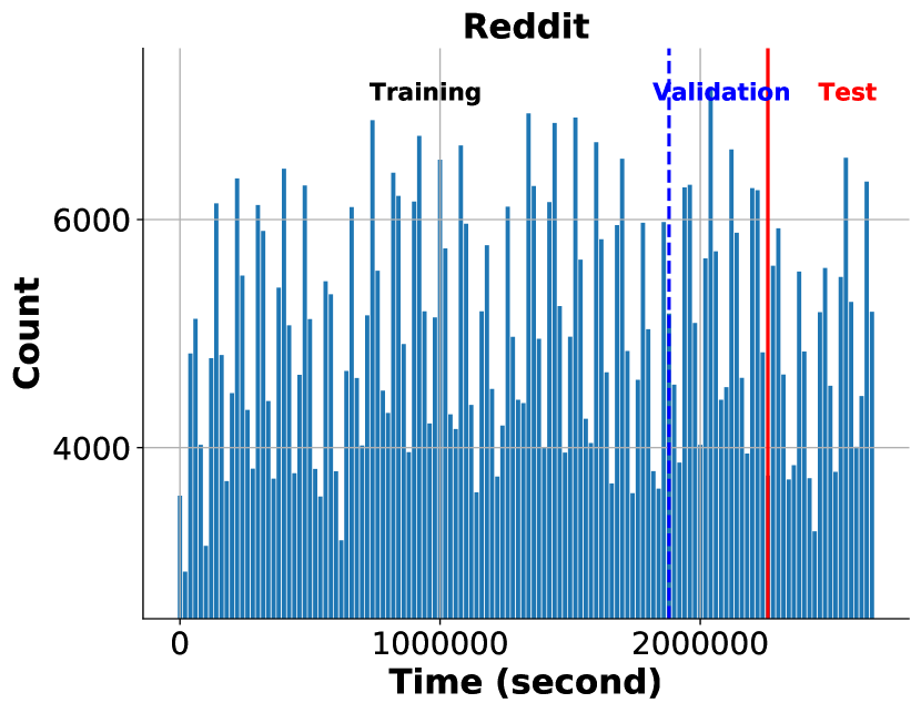
As shown in Table 2 of the main paper, we select fifteen benchmark databases from diverse domains. All datasets are publicly available under CC BY-NC licence and can be accessed at https://drive.google.com/drive/folders/1HKSFGEfxHDlHuQZ6nK4SLCEMFQIOtzpz?usp=sharing. Figure 5 shows the temporal distribution of edges in the evaluated temporal graphs.

•

Reddit is a bipartite interaction graph, consisting of one month of posts made by users on subreddits [9]. Users and subreddits are nodes, and egdes are interactions of users writing posts to subreddits. The text of each post is converted into LIWC-feature vector [32] as an edge feature of length 172. This public dataset gives 366 true labels among 672,447 interactions, and those true label are ground-truth labels of banned users from Reddit [1].
•

Wikipedia is a bipartite interaction graph, and contains one month of edits made by editors. This public dataset selects the 1,000 most edited pages as items and editors who made at least 5 edits as users over a month [1]. Editors and pages are nodes, and edges are interactions of editors editing on pages. Edge features of length 172 are interaction edits converted into LIWC-feature vectors [32]. Wikipedia dataset treats 217 public ground-truth labels of banned users from 157,474 interactions as positive labels.
•

MOOC is a bipartite MOOC online network of students and online course content units [10]. Students and courses are nodes, and edges with features of length 4 are interactions of user viewing a video, submitting an answer, etc. This public dataset treats 4,066 dropout events out of 411,749 interactions as positive labels [1].
•

LastFM is a user-song bipartite network [11]. Users and songs are nodes, and edges are user-listens-song interactions. This public dataset includes 1,293,103 interactions between all 1000 users and the 1000 most listened songs [1].
•

Enron is an email communication network that collects about half a million emails over several years [13]. Nodes of the network are email addresses, and edges are email communication between accounts [14].
•

SocialEvo is a network in which experiments are conducted to closely track the everyday life of a whole undergraduate dormitory with mobile phones. This public dataset is collected by a cell phone application every six minutes, and contains physical proximity and location between students living in halls of residence. [15].
•

UCI is a facebook-like social network that contains user posts to forums. Nodes are students (1,899) at University of California, Irvine, and edges are interactions of online messages (59,835) among these users [16]. Each edge has 100 features.
•

CollegeMsg is provided by the SNAP team of Stanford [17]. This dataset is derived from the facebook-like social network introduced in dataset UCI. The SNAP team has parsed it to a temporal network. Each edge has 172 features.

(a) Reddit

(b) Wikipedia

(c) MOOC

(d) LastFM

(e) Enron

(f) SocialEvo

(g) UCI

(h) CollegeMsg

(i) CanParl

(j) Contact

(k) Flights

(l) UNTrade

(m) USLegis

(n) UNVote

(o) Taobao

Figure 5: The temporal distribution of edges of the evaluated temporal graphs.
•

CanParl is a Canadian parliament bill voting network extracted from open website [18]. Nodes are members of parliament (MPs), and edges are the interactions between MPs from 2006 to 2019.
•

Contact is a temporal and weighted network of physical proximity among the participants [19]. Nodes are participant and edges are proximity events between the study participants. Edge features indicate the physical proximity between participants [8].
•

Flights is a weighted flight network. Nodes are airports, and edges are tracked flights [20]. The weights of edges indicate the number of flights between two given airports within a day [8].
•

UNTrade is a food and agriculture trading weighted network among 181 nations over 30 years [21]. Nodes are countries, and edges are tradings between two countries. The weights of edges are the total sum of normalized agriculture import or export values between two given countries [8].
•

USLegis is a senate co-sponsorship network that examines the social relations of legislators in their co-sponsorship relationships on bills [18]. Nodes are congress members, and edge weights are the number of times that two members of congress co-sponsor a bill in a given congress [8].
•

UNVote is a weighted network of roll-call votes in the UN General Assembly 1946-2021 [22]. Nodes are nations, and edge weights are the number of times both nations have voted "yes" to an item.
•

Taobao is a subset of the Taobao user behavior dataset intercepted based on the period 8:00 to 18:00 on 26 November 2017 [12]. This public dataset is a user-item bipartite network. Nodes are users and items, and edges are behaviors between users and items, such as favor, click, purchase, and add an item to shopping cart. Each edge has 4 features, corresponding to 4 different types of behaviors [6].

Appendix B Experiment Details

DataLoader of the link prediction pipeline introduced in Section 3.2.1 splits and generates training set, validation set, transductive set, and inductive test sets depending on the New-Old and New-New settings, for link prediction task. The detailed statistics of these data sets are shown in Table 6. DataLoader of the node classification pipeline introduced in Section 3.2.2 follows the traditional transductive setting. The detailed statistics of the training set, validation set, and test set on three available datasets (Reddit, Wikipedia, and MOOC) are given in Table 7.

Table 6: Statistics of datasets for link prediction task. "New-Old Validation" indicates the validation set under Inductive New-Old setting, and so on.

	Training		Validation		Transductive Test		Inductive Validation		Inductive Test
	# nodes	# edges	# nodes	# edges	# nodes	# edges	# nodes	# edges	# nodes	# edges
Reddit	9,574	389,989	9,839	100,867	9,615	100,867	3,491	19,446	3,515	21,470
Wikipedia	6,141	81,029	3,256	23,621	3,564	23,621	2,120	12,016	2,437	11,715
MOOC	6,015	227,485	2,599	61,762	2,412	61,763	2,333	25,592	2,181	29,179
LastFM	1,612	722,758	1,714	193,965	1,753	193,966	1,643	57,651	1,674	98,442
Enron	157	79,064	155	18,786	141	18,785	112	5,637	110	4,859
SocialEvo	67	1,222,980	64	314,930	62	314,924	62	62,811	60	70,038
UCI	1,338	34,386	1,036	8,975	847	8,976	816	4,761	678	5,707
CollegeMsg	1,337	34,544	1,036	8,975	847	8,975	818	4,914	680	5,885
CanParl	618	47,435	344	11,809	342	10,113	344	5,481	341	5,591
Contact	617	1,372,030	632	364,005	629	363,780	582	68,261	590	69,617
Flights	11,230	1,107,798	10,844	279,399	10,906	287,824	6,784	54,861	6,820	58,102
UNTrade	230	291,287	230	78,721	228	61,595	227	17,528	226	14,001
USLegis	176	38,579	113	10,005	100	4,950	113	5,010	100	3,297
UNVote	178	600,511	194	135,298	194	155,119	194	28,136	194	33,083
Taobao	54,462	45,630	17,964	11,621	18,143	11,550	16,476	10,338	16,896	10,516
	New-Old Validation		New-Old Test		New-New Validation		New-New Test		Unseen Nodes
	# nodes	# edges	# nodes	# edges	# nodes	# edges	# nodes	# edges	Unseen Nodes
Reddit	3,301	16,760	3,325	18,703	488	2,686	486	2,767	1,098
Wikipedia	1,809	8,884	1,996	8,148	468	3,132	629	3,567	922
MOOC	2,316	23,109	2,164	25,730	553	2,483	592	3,449	714
LastFM	1,642	52,379	1,674	63,505	272	5,272	331	34,937	198
Enron	111	4,965	109	4,262	19	672	20	597	18
SocialEvo	62	58,959	60	65,466	7	3,852	7	4,572	7
UCI	757	3,686	606	4,193	247	1,075	213	1,514	189
CollegeMsg	759	3,839	608	4,328	247	1,075	214	1,557	189
CanParl	344	4,543	341	4,469	106	938	111	1,122	73
Contact	582	64,887	590	65,883	62	3,374	59	3,734	69
Flights	6,711	49,796	6,739	52,504	874	5,065	937	5,598	1,316
UNTrade	227	16,420	226	13,112	25	1,108	25	889	25
USLegis	112	4,154	100	2,436	37	856	42	861	22
UNVote	194	26,545	194	31,166	23	1,591	23	1,917	20
Taobao	9,247	5,678	8,136	4,860	7,706	4,660	9,298	5,656	8,256

Table 7: Statistics of datasets for node classification task.

	Training		Validation		Test
	# nodes	# edges	# nodes	# edges	# nodes	# edges
Reddit	10,844	470,713	9,839	100,867	9,615	100,867
Wikipedia	7,475	110,232	3,256	23,621	3,564	23,621
MOOC	6,625	288,224	2,599	61,762	2,412	61,763

EdgeSampler of link prediction pipeline introduced in Section 3.2.1 uses fixed seeds for different validation sets and test sets to ensure that the test results are reproducible across different runs.

Table 8: Experimental parameters of TGAT.

	$d_{n}$	$d_{e}$	$d_{time}$	$d_{pos}$	$n_{head}$
Reddit	172	172	172	172	2
Wikipedia	172	172	172	172	2
MOOC	172	4	172	172	2
LastFM	172	2	172	172	2
Enron	172	32	172	172	2
SocialEvo	172	2	172	172	2
UCI	172	100	172	172	2
CollegeMsg	172	172	172	172	2
CanParl	172	1	172	172	1
Contact	172	1	172	172	1
Flights	172	1	172	172	1
UNTrade	172	1	172	172	1
USLegis	172	1	172	172	1
UNVote	172	1	172	172	1
Taobao	172	4	172	172	2

Table 9: Experimental parameters of CAWN.

	$d_{n}$	$d_{e}$	$d_{time}$	$d_{pos}$
Reddit	172	172	172	108
Wikipedia	172	172	172	108
MOOC	172	4	172	100
LastFM	172	2	172	102
Enron	172	32	172	104
SocialEvo	172	2	172	102
UCI	172	100	172	100
CollegeMsg	172	172	172	108
CanParl	172	1	172	103
Contact	172	1	172	103
Flights	172	1	172	103
UNTrade	172	1	172	103
USLegis	172	1	172	103
UNVote	172	1	172	103
Taobao	172	4	172	100

Appendix C Model Implementation Details

We implement JODIE, DyRep, and TGN based on the TGN framework. Furthermore, we fix the inconsistencies of implementations between link prediction task and node classification task.

TGAT concatenates node features, edge features, time features, and position features to perform the multi-head self-attention mechanism. There is a positional encoding in the self-attention mechanism for capturing sequential information. Let $d_{n}$ , $d_{e}$ , $d_{time}$ , and $d_{pos}$ denote the dimensions of node features, edge features, time features, and positional encoding, respectively. The number of attention heads is $n_{head}$ . These parameters must satisfy:

(d_{n}+d_{e}+d_{time}+d_{pos})\%n_{head}=0

(1)

The experimental parameters of TGAT are summarized in Table 9.

Similar to the setup of TGAT, CAWN adopts a multi-head self-attention mechanism to capture the subtle relevance of node features, edge features, time features, and positional features. Those parameters satisfy Formula (1) as well, and $d_{n}=d_{time}$ . However, CAWN initializes the number of attention heads to 2, so we change the dimension of $d_{pos}$ to conduct experiments. The experimental parameters of CAWN are shown in Table 9.

NeurTW concatenates node features, edge features, and positional features (without time features) during the temporal random walk encoding. Regarding the temporal walk sampling strategy, given a node $u$ at time $t$ , the sampling probability weight of its neighbor $v$ ( $(\{v,u\},t^{\prime})\in\mathcal{G}_{u,t}$ ) is proportion to $exp(\alpha(t^{\prime}-t))$ , where $\alpha$ is a temporal bias. This sampling strategy is a temporal-biased sampling method. However, the time intervals in some benchmark datasets (Enron, CanParl, UNTrade, USLegis, and UNVote) are relatively large, and the exponential sampling probability weights may encounter overflow. Therefore, we propose a strategy to calculate the sampling probability weights for these datasets:

W(v,t^{\prime})=\begin{cases}t^{\prime}-t,&t^{\prime}-t>0,\\ 1,&t^{\prime}-t=0,\\ -1/(t^{\prime}-t),&t^{\prime}-t<0,\end{cases}

(2)

where $W(v,t^{\prime})>0$ . This strategy can avoid overflow and is also a temporal-biased sampling method. Finally, the sampling probability of each neighbor is obtained after normalization:

Pr_{t}(v)=\frac{\alpha W(v,t_{v})}{\sum_{v^{\prime}\in\mathcal{G}_{u,t}}\alpha W(v^{\prime},t_{v^{\prime}})},

(3)

where $\alpha$ is a temporal bias. For other hyperparameters that we have not mentioned, we use default values from the original experiments in the corresponding papers. All the experimental codes are publicly available under MIT license and can be accessed at https://github.com/qianghuangwhu/benchtemp.

Appendix D Experiment Results

Table 10: Average Precision (AP) results on link prediction task. "*" denotes that the model encounters runtime error; "—" denotes timeout after 48 hours. The best and second-best results are highlighted as bold red and underlined blue. Some standard deviations are zero because we terminate those models that can only run one epoch within 2 days. We do not highlight the second-best if the gap is

>0.05

compared with the best result.

	Transductive
	JODIE	DyRep	TGN	TGAT	CAWN	NeurTW	NAT
Reddit	0.9718 ± 0.0022	0.9808 ± 0.0006	0.9874 ± 0.0002	0.9822 ± 0.0003	0.9904 ± 0.0001	0.9855 ± 0.0013	0.9868 ± 0.0017
Wikipedia	0.9471 ± 0.0056	0.9464 ± 0.0010	0.9852 ± 0.0003	0.9536 ± 0.0022	0.9906 ± 0.0001	0.9918 ± 0.0001	0.9819 ± 0.0026
MOOC	0.7364 ± 0.0370	0.7933 ± 0.0348	0.883 ± 0.0242	0.7185 ± 0.0051	0.9369 ± 0.0009	0.7943 ± 0.0248	0.7537 ± 0.0191
LastFM	0.6762 ± 0.0678	0.6736 ± 0.0768	0.7694 ± 0.0276	0.5375 ± 0.0044	0.8946 ± 0.0006	0.8405 ± 0.0	0.8729 ± 0.0022
Enron	0.7841 ± 0.0254	0.7648 ± 0.0418	0.8472 ± 0.0173	0.6063 ± 0.0194	0.9142 ± 0.0052	0.8847 ± 0.0079	0.9044 ± 0.0036
SocialEvo	0.7982 ± 0.0476	0.8816 ± 0.0042	0.9325 ± 0.0006	0.7724 ± 0.0052	0.9188 ± 0.0011	—	0.8989 ± 0.0096
UCI	0.8436 ± 0.0110	0.4913 ± 0.0367	0.8914 ± 0.0138	0.779 ± 0.0052	0.9425 ± 0.001	0.9702 ± 0.0021	0.9253 ± 0.0083
CollegeMsg	0.5276 ± 0.0493	0.5070 ± 0.0049	0.8418 ± 0.0847	0.7902 ± 0.0033	0.9401 ± 0.0025	0.9727 ± 0.0001	0.9241 ± 0.0086
CanParl	0.7030 ± 0.0077	0.6860 ± 0.0256	0.6765 ± 0.0615	0.6811 ± 0.0157	0.6916 ± 0.0546	0.8528 ± 0.0213	0.6593 ± 0.0764
Contact	0.9087 ± 0.0114	0.9016 ± 0.0319	0.9699 ± 0.0045	0.5888 ± 0.0065	0.9677 ± 0.0024	0.9756 ± 0.0	0.945 ± 0.0168
Flights	0.9389 ± 0.0075	0.8836 ± 0.0078	0.9764 ± 0.0025	0.899 ± 0.0025	0.9860 ± 0.0002	0.9321 ± 0.0	0.9749 ± 0.0048
UNTrade	0.6329 ± 0.0102	0.6099 ± 0.0057	0.6059 ± 0.0086	*	0.7488 ± 0.0005	0.5648 ± 0.0167	0.7514 ± 0.0615
USLegis	0.7585 ± 0.0032	0.6808 ± 0.0368	0.7398 ± 0.0027	0.7206 ± 0.0071	0.9682 ± 0.0048	0.9713 ± 0.0013	0.7425 ± 0.016
UNVote	0.6090 ± 0.0076	0.5855 ± 0.0225	0.6694 ± 0.0095	0.5388 ± 0.002	0.6175 ± 0.0013	0.6008 ± 0.0	0.6449 ± 0.033
Taobao	0.808 ± 0.0015	0.8074 ± 0.0014	0.8618 ± 0.0004	0.5508 ± 0.0093	0.7464 ± 0.0027	0.8808 ± 0.0012	0.8933 ± 0.0007
	Inductive
	JODIE	DyRep	TGN	TGAT	CAWN	NeurTW	NAT
Reddit	0.9427 ± 0.0118	0.9582 ± 0.0003	0.9767 ± 0.0003	0.9667 ± 0.0003	0.9889 ± 0.0001	0.9821 ± 0.0006	0.9912 ± 0.0027
Wikipedia	0.9316 ± 0.0049	0.9181 ± 0.0037	0.9791 ± 0.0004	0.9389 ± 0.0035	0.9903 ± 0.0002	0.9912 ± 0.0004	0.9962 ± 0.0021
MOOC	0.7282 ± 0.0686	0.7985 ± 0.0153	0.8726 ± 0.0267	0.7204 ± 0.0055	0.9394 ± 0.0005	0.7903 ± 0.0307	0.7474 ± 0.0214
LastFM	0.8057 ± 0.0424	0.7956 ± 0.0631	0.8261 ± 0.0145	0.5454 ± 0.0094	0.9225 ± 0.0009	0.8842 ± 0.0	0.9235 ± 0.0028
Enron	0.7640 ± 0.0310	0.6883 ± 0.0635	0.7982 ± 0.0237	0.5661 ± 0.0134	0.916 ± 0.001	0.8940 ± 0.0025	0.9308 ± 0.0085
SocialEvo	0.8527 ± 0.0303	0.8954 ± 0.0034	0.8944 ± 0.0102	0.6497 ± 0.004	0.9118 ± 0.0003	—	0.8682 ± 0.0324
UCI	0.7298 ± 0.0152	0.4606 ± 0.0209	0.8306 ± 0.0177	0.704 ± 0.0046	0.9421 ± 0.0012	0.9720 ± 0.0024	0.9658 ± 0.0125
CollegeMsg	0.4960 ± 0.0193	0.4858 ± 0.0051	0.7983 ± 0.049	0.7184 ± 0.0014	0.941 ± 0.0026	0.9762 ± 0.0	0.9642 ± 0.0124
CanParl	0.5148 ± 0.0119	0.5365 ± 0.0064	0.5596 ± 0.0141	0.5814 ± 0.0041	0.6915 ± 0.0578	0.8469 ± 0.0161	0.6058 ± 0.0812
Contact	0.9162 ± 0.0051	0.8334 ± 0.0620	0.9411 ± 0.0071	0.5922 ± 0.0056	0.9688 ± 0.0023	0.9762 ± 0.0	0.9489 ± 0.0091
Flights	0.9190 ± 0.0081	0.8707 ± 0.0121	0.9439 ± 0.0043	0.8361 ± 0.0039	0.9834 ± 0.0002	0.9201 ± 0.0	0.9817 ± 0.0026
UNTrade	0.6392 ± 0.0132	0.6232 ± 0.0188	0.5603 ± 0.0106	*	0.7361 ± 0.0009	0.5640 ± 0.0137	0.6586 ± 0.0543
USLegis	0.5557 ± 0.0107	0.5687 ± 0.0008	0.6048 ± 0.0047	0.5637 ± 0.0048	0.9694 ± 0.0028	0.971 ± 0.0009	0.6946 ± 0.0198
UNVote	0.5242 ± 0.0050	0.5118 ± 0.0037	0.5702 ± 0.0099	0.5204 ± 0.004	0.6014 ± 0.0013	0.6025 ± 0.0	0.7637 ± 0.0023
Taobao	0.6696 ± 0.0025	0.6717 ± 0.0006	0.6761 ± 0.0015	0.5293 ± 0.0096	0.7389 ± 0.0026	0.8815 ± 0.0045	0.9992 ± 0.0001
	Inductive New-Old
	JODIE	DyRep	TGN	TGAT	CAWN	NeurTW	NAT
Reddit	0.9399 ± 0.0112	0.9552 ± 0.0027	0.9749 ± 0.0006	0.9659 ± 0.0004	0.9871 ± 0.0003	0.9810 ± 0.0015	0.9947 ± 0.0014
Wikipedia	0.9127 ± 0.0078	0.8947 ± 0.0040	0.9724 ± 0.0008	0.9223 ± 0.0021	0.9901 ± 0.0002	0.9884 ± 0.0007	0.9959 ± 0.0018
MOOC	0.7366 ± 0.5977	0.8011 ± 0.0092	0.8669 ± 0.0328	0.7263 ± 0.0059	0.9408 ± 0.0022	0.7907 ± 0.0336	0.7677 ± 0.0175
LastFM	0.7448 ± 0.0034	0.7024 ± 0.0532	0.7661 ± 0.0232	0.5447 ± 0.0023	0.8906 ± 0.0021	0.835 ± 0.0	0.9235 ± 0.001
Enron	0.7526 ± 0.0158	0.6742 ± 0.0632	0.7918 ± 0.0209	0.5729 ± 0.0189	0.9168 ± 0.0061	0.8925 ± 0.0090	0.9319 ± 0.0092
SocialEvo	0.8521 ± 0.0403	0.8999 ± 0.0046	0.8972 ± 0.0107	0.6578 ± 0.0041	0.8830 ± 0.0008	—	0.8437 ± 0.0569
UCI	0.6891 ± 0.0166	0.4574 ± 0.0207	0.8243 ± 0.0205	0.6826 ± 0.0084	0.9414 ± 0.002	0.9732 ± 0.0040	0.9768 ± 0.0127
CollegeMsg	0.5000 ± 0.0227	0.4834 ± 0.0177	0.7954 ± 0.0349	0.701 ± 0.0058	0.9407 ± 0.0017	0.9719 ± 0.0014	0.9763 ± 0.0133
CanParl	0.5143 ± 0.0043	0.5168 ± 0.0170	0.552 ± 0.0135	0.574 ± 0.0054	0.6952 ± 0.0518	0.8417 ± 0.0132	0.6027 ± 0.0787
Contact	0.9150 ± 0.0058	0.8253 ± 0.0637	0.9421 ± 0.0055	0.5915 ± 0.0049	0.9689 ± 0.0029	0.9757 ± 0.0	0.9384 ± 0.0175
Flights	0.9128 ± 0.0095	0.8657 ± 0.0117	0.9412 ± 0.0039	0.833 ± 0.0031	0.9827 ± 0.0002	0.9161 ± 0.0	0.9845 ± 0.0033
UNTrade	0.6333 ± 0.0102	0.6101 ± 0.0196	0.5622 ± 0.014	*	0.7375 ± 0.001	0.5692 ± 0.0185	0.5844 ± 0.053
USLegis	0.5567 ± 0.0106	0.5490 ± 0.0143	0.5651 ± 0.0131	0.5695 ± 0.0099	0.9703 ± 0.0027	0.9671 ± 0.0027	0.5024 ± 0.0511
UNVote	0.5348 ± 0.0072	0.5126 ± 0.0103	0.5724 ± 0.0107	0.5196 ± 0.0022	0.6050 ± 0.0019	0.6036 ± 0.0	0.7598 ± 0.0167
Taobao	0.6838 ± 0.0045	0.6884 ± 0.0013	0.6944 ± 0.0038	0.5309 ± 0.0189	0.7374 ± 0.0032	0.8687 ± 0.0010	0.9997 ± 0.0001
	Inductive New-New
	JODIE	DyRep	TGN	TGAT	CAWN	NeurTW	NAT
Reddit	0.9199 ± 0.0167	0.9384 ± 0.0064	0.9727 ± 0.0004	0.9523 ± 0.0056	0.9958 ± 0.0017	0.9890 ± 0.0003	0.9951 ± 0.0005
Wikipedia	0.9307 ± 0.0060	0.9329 ± 0.0028	0.9822 ± 0.0009	0.9592 ± 0.0039	0.9941 ± 0.0004	0.9963 ± 0.0003	0.9979 ± 0.0009
MOOC	0.6623 ± 0.0189	0.7135 ± 0.0148	0.8651 ± 0.0059	0.7239 ± 0.0052	0.935 ± 0.0009	0.7871 ± 0.0221	0.6654 ± 0.0155
LastFM	0.8558 ± 0.0110	0.8388 ± 0.0209	0.8121 ± 0.0046	0.536 ± 0.0217	0.9716 ± 0.0008	0.9585 ± 0.0	0.9722 ± 0.0013
Enron	0.6525 ± 0.0146	0.6312 ± 0.0449	0.7391 ± 0.0196	0.538 ± 0.0093	0.9556 ± 0.0055	0.9358 ± 0.0008	0.9503 ± 0.0079
SocialEvo	0.5958 ± 0.0391	0.7312 ± 0.0103	0.8268 ± 0.003	0.5096 ± 0.0097	0.9150 ± 0.0013	—	0.9112 ± 0.0563
UCI	0.6249 ± 0.0198	0.5062 ± 0.0032	0.8393 ± 0.0155	0.7758 ± 0.0033	0.9488 ± 0.0012	0.9736 ± 0.0008	0.9518 ± 0.0211
CollegeMsg	0.5212 ± 0.0244	0.5328 ± 0.0117	0.8244 ± 0.0098	0.7929 ± 0.0029	0.9484 ± 0.0039	0.9797 ± 0.0008	0.95 ± 0.0257
CanParl	0.4697 ± 0.0043	0.4794 ± 0.0057	0.5553 ± 0.0258	0.6004 ± 0.0087	0.6671 ± 0.0795	0.8511 ± 0.0079	0.5989 ± 0.0571
Contact	0.7381 ± 0.0145	0.6601 ± 0.0432	0.8916 ± 0.0075	0.5779 ± 0.0044	0.9670 ± 0.0031	0.9704 ± 0.0	0.9535 ± 0.0044
Flights	0.9250 ± 0.0065	0.6312 ± 0.0449	0.9644 ± 0.0015	0.8608 ± 0.0049	0.9882 ± 0.0009	0.9496 ± 0.0	0.9906 ± 0.0009
UNTrade	0.5801 ± 0.0112	0.5344 ± 0.0130	0.5164 ± 0.0056	*	0.7404 ± 0.0023	0.5685 ± 0.0298	0.6785 ± 0.0289
USLegis	0.5250 ± 0.0045	0.5523 ± 0.0127	0.5582 ± 0.02	0.5434 ± 0.0203	0.9767 ± 0.0055	0.9803 ± 0.0005	0.8627 ± 0.0196
UNVote	0.4973 ± 0.0145	0.4856 ± 0.0078	0.5502 ± 0.0096	0.5337 ± 0.0046	0.5830 ± 0.0076	0.5964 ± 0.0	0.7549 ± 0.035
Taobao	0.6764 ± 0.0013	0.676 ± 0.0011	0.6739 ± 0.0016	0.5222 ± 0.0033	0.7390 ± 0.0147	0.9025 ± 0.0035	0.9997 ± 0.0001

D.1 AP Results for Link Prediction

We show the average precision (AP) results on link prediction task and highlight the best and second-best numbers for each job in Table 10. The overall performance is similar to that of AUC. For the transductive setting, CAWN gives impressive results and achieves the best or second-best results on 12 datasets out of 15, followed by NeurTW (7 out of 15), TGN (5 out of 15), and NAT (5 out of 15), verifying the effectiveness of temporal walk, temporal memory, and joint neighborhood on transductive link prediction task. For the inductive setting, CAWN and NAT both rank top-2 on 9 datasets, followed by NeurTW on 6. Results reveal that models based on temporal walks and joint neighborhood can better capture structure patterns on edges that have never been seen. TGN performs relatively poorly for the inductive link prediction task on almost all datasets. We can draw similar conclusions from inductive New-Old and inductive New-Old experimental results. We note that DyRep achieves the best AP result under the inductive New-Old setting and the second-best AP result under the inductive setting on the SocialEvo dataset. SocialEvo has the maximum average degree and edge density as shown in Table 2 in the main paper, demonstrating that DyRep performs better for inductive link prediction tasks on dense temporal graphs.

D.2 GPU Utilization Comparison for Link Prediction

In Table 11, we report the GPU utilization results on the link prediction task. NAT obtains the best or second-best results on 13 datasets out of 15, followed by TGN (9 out of 15). The data structure, called N-cache, designed in NAT supports parallel access and updates of dictionary-type neighborhood representation on GPUs. Therefore, NAT achieves the best performance regarding GPU utilization. TGN proposes a highly efficient parallel processing strategy to handle temporal graph, so that TGN has the second-best performance on GPU utilization.

Table 11: GPU utilization of models on link prediction task. "*" denotes that TGAT layer cannot find suitable neighbors within given time interval and encounters error. The best and second-best results are highlighted as bold red and underlined blue.

	GPU Utilization (%)
	JODIE	DyRep	TGN	TGAT	CAWN	NeurTW	NAT
Reddit	21	22	41	39	26	31	40
Wikipedia	34	46	36	35	28	17	38
MOOC	14	29	35	35	18	14	45
LastFM	22	28	38	22	23	22	48
Enron	18	24	41	24	25	22	51
SocialEvo	24	25	42	25	17	22	46
UCI	30	25	35	33	27	58	44
CollegeMsg	21	32	46	47	25	34	48
CanParl	26	27	54	47	24	22	51
Contact	25	22	40	29	19	22	50
Flights	20	20	26	35	18	24	43
UNTrade	19	23	50	*	15	23	53
USLegis	22	28	54	38	26	55	53
UNVote	12	22	37	35	16	46	54
Taobao	29	56	31	55	22	53	38

D.3 Efficiency Comparison of Node Classification Task

Table 12: Model efficiency on the node classification task. We report seconds per epoch as Runtime, the averaged number of epochs for convergence before early stopping as Epoch, the maximum RAM usage as RAM, the maximum GPU memory usage as GPU Memory, and the maximum GPU utilization usage as GPU Utilization, respectively. "x" indicates that the model cannot converge within 48 hours. The best and second-best results are highlighted as bold red and underlined blue.

	Runtime (second)							Epoch
	JODIE	DyRep	TGN	TGAT	CAWN	NeurTW	NAT	JODIE	DyRep	TGN	TGAT	CAWN	NeurTW	NAT
Reddit	65.98	75.07	73.99	16.99	1,913.83	24,016.13	28.24	6	7	8	4	x	x	6
Wikipedia	15.75	14.55	14.58	4.95	351.54	2,723.37	6.39	4	14	3	7	6	4	3
MOOC	28.57	32.91	27.95	8.51	1,146.76	7,466.04	17.55	8	3	5	7	10	x	3
	RAM (GB)							GPU Memory (GB)
Reddit	3.8	3.4	3.3	4.1	45.7	16.7	3.3	2.9	2.8	3.1	3.0	3.7	3.0	3.0
Wikipedia	2.6	2.6	2.6	3.1	8.2	8.2	2.6	2.6	2.4	2.8	2.5	3.1	2.5	1.7
MOOC	2.9	2.9	2.9	3.1	45.1	32.6	2.5	1.9	1.8	1.9	2.1	2.3	1.7	1.3
	GPU Utilization (%)
Reddit	41	40	42	38	18	36	52
Wikipedia	37	30	41	31	25	80	48
MOOC	35	33	40	30	13	56	62

We compare the efficiency results on node classification task and show the results in Table 12. Regarding runtime per epoch, TGAT achieves the fastest performance on all three datasets, followed by NAT. Similar to the runtime results on the link prediction task, the training process of CAWN and NeurTW is much slower due to the inefficient temporal walk. As for the averaged number of epochs for convergence, NAT ranks top-2 on all three datasets, followed by JODIE (2 out of 3), TGN (2 out of 3). RAM results reveal that CAWN and NeurTW consume much more memory due to the temporal walk and complex sampling strategy. Most models need 1 - 3 GB of GPU memory, similar to the link prediction task. Due to the parallel access and update of representation on GPU, NAT achieves the highest GPU utilization.

Appendix E Results of TeMP

Upon the anatomy of the existing methods, we propose a novel temporal graph neural network, called TeMP. As shown in Figure 6, given a dynamic graph (a), the processing of TeMP is as follows:

•

Subgraph Construction (b). We construct a subgraph with a temporal neighbor sampler with intervals adaptive to data. We try to find a reference timestamp and sample a subgraph before this timestamp. We have conducted experiments at various quantiles, and chosen the mean timestamp since it obtains the overall best performance.
•

Embedding Generation (c). Upon subgraph construction, TeMP generates temporal embeddings for nodes and edges. The model architecture consists of three main components: temporal label propagation (LPA), message-passing operators, and a sequence updater. The temporal LPA captures the motif pattern, while the message-passing operators aggregate the original edge features. The sequence updater chooses RNN to update the embeddings with a memory module. Furthermore, TeMP uses a pre-initialization strategy to generate initial temporal node embeddings.

Table 13: AUC and AP results of TeMP on link prediction task. We highlight the numbers as bold red and underlined blue if TeMP achieves the best and second-best results compared to the TGNN models in the main paper.

	AUC
	Transductive	Inductive	Inductive New-Old	Inductive New-New
Reddit	0.99 ± 0.0001	0.9843 ± 0.0002	0.9818 ± 0.0001	0.9843 ± 0.0003
Wikipedia	0.9801 ± 0.0005	0.9669 ± 0.0008	0.9504 ± 0.0005	0.97 ± 0.0013
MOOC	0.8249 ± 0.0027	0.8277 ± 0.0036	0.832 ± 0.0031	0.7621 ± 0.0086
LastFM	0.865 ± 0.0012	0.8879 ± 0.0015	0.8333 ± 0.0014	0.9228 ± 0.0007
Enron	0.8717 ± 0.0122	0.8485 ± 0.0153	0.8491 ± 0.009	0.7798 ± 0.0329
SocialEvo	0.9303 ± 0.0005	0.9039 ± 0.0005	0.9017 ± 0.0013	0.8485 ± 0.0041
UCI	0.8925 ± 0.001	0.7955 ± 0.0054	0.7787 ± 0.0032	0.7318 ± 0.0017
CollegeMsg	0.8873 ± 0.0018	0.8027 ± 0.0029	0.7848 ± 0.0022	0.7342 ± 0.0047
CanParl	0.7801 ± 0.0139	0.5414 ± 0.0176	0.5313 ± 0.0253	0.5683 ± 0.0293
Contact	0.958 ± 0.0013	0.9474 ± 0.0015	0.9474 ± 0.0011	0.7835 ± 0.0041
Flights	0.987 ± 0.0003	0.9708 ± 0.0006	0.9692 ± 0.0006	0.973 ± 0.0009
UNTrade	0.6011 ± 0.0009	0.5732 ± 0.0006	0.5703 ± 0.0006	0.5539 ± 0.0008
USLegis	0.7073 ± 0.0114	0.5493 ± 0.0183	0.5609 ± 0.0123	0.5425 ± 0.0234
UNVote	0.5571 ± 0.0053	0.5419 ± 0.006	0.5409 ± 0.0066	0.5696 ± 0.0038
Taobao	0.939 ± 0.0005	0.8513 ± 0.0018	0.8249 ± 0.003	0.8502 ± 0.0025
	AP
	Transductive	Inductive	Inductive New-Old	Inductive New-New
Reddit	0.9904 ± 0.0001	0.9849 ± 0.0002	0.9828 ± 0.0002	0.9757 ± 0.0007
Wikipedia	0.9817 ± 0.0004	0.9696 ± 0.0004	0.9562 ± 0.0005	0.9666 ± 0.0016
MOOC	0.7935 ± 0.0033	0.7918 ± 0.0039	0.7989 ± 0.0035	0.7328 ± 0.0089
LastFM	0.8717 ± 0.0014	0.8952 ± 0.0015	0.8468 ± 0.0015	0.8984 ± 0.0014
Enron	0.85 ± 0.0141	0.8274 ± 0.0167	0.8324 ± 0.0104	0.757 ± 0.0307
SocialEvo	0.9098 ± 0.0005	0.8767 ± 0.0004	0.8752 ± 0.0021	0.7907 ± 0.0056
UCI	0.8968 ± 0.0007	0.8104 ± 0.0054	0.7969 ± 0.0047	0.7594 ± 0.0047
CollegeMsg	0.8928 ± 0.0026	0.8206 ± 0.0041	0.8018 ± 0.003	0.7505 ± 0.0045
CanParl	0.6871 ± 0.015	0.5388 ± 0.0074	0.5341 ± 0.0037	0.5554 ± 0.015
Contact	0.9525 ± 0.0016	0.9429 ± 0.0019	0.944 ± 0.0012	0.7992 ± 0.0031
Flights	0.9857 ± 0.0003	0.9687 ± 0.0005	0.9661 ± 0.0006	0.9731 ± 0.001
UNTrade	0.5855 ± 0.0007	0.564 ± 0.0007	0.5593 ± 0.0011	0.5634 ± 0.0008
USLegis	0.6493 ± 0.0078	0.529 ± 0.01	0.5519 ± 0.0088	0.5375 ± 0.0218
UNVote	0.5402 ± 0.0038	0.536 ± 0.005	0.5354 ± 0.0041	0.5481 ± 0.0052
Taobao	0.9385 ± 0.0004	0.8493 ± 0.0033	0.8243 ± 0.0049	0.8448 ± 0.0056

Table 14: Efficiency of TeMP on link prediction task.

	Efficiency
	Runtime (second)	Epoch	RAM (GB)	GPU Memory (GB)	GPU Utilization (%)
Reddit	304.84	27	5.4	2.3	86
Wikipedia	51.00	22	3.4	1.4	71
MOOC	100.64	23	2.9	1.3	57
LastFM	471.25	48	3.6	1.4	57
Enron	38.68	20	2.8	1.1	31
SocialEvo	670.08	30	3.77	1.1	30
UCI	43.98	26	2.9	1.4	50
CollegeMsg	11.55	30	3	1.2	49
CanParl	13.80	7	2.8	1.1	37
Contact	421.15	54	4.1	1.3	13
Flights	859.04	38	3.9	1.4	76
UNTrade	80.96	10	3	1.3	37
USLegis	10.31	14	2.6	1.1	57
UNVote	165.32	12	3.3	1.3	39
Taobao	17.78	16	3.1	1.5	42

Table 15: AUC and efficiency results of TeMP on node classification task.

	AUC	Efficiency
	AUC	Runtime (second)	Epoch	RAM (GB)	GPU Memory (GB)	GPU Utilization (%)
Reddit	0.6357 ± 0.0265	170.66	7	4.4	3.0	66
Wikipedia	0.8873 ± 0.0078	24.18	13	3.5	1.4	47
MOOC	0.6958 ± 0.0017	49.90	7	3.3	1.2	42

E.1 Experimental Results

Link Prediction. The AUC and AP results of TeMP on link prediction task are presented in Table 13, and the efficiency results are shown in Table 14. TeMP performs relatively well in the transductive setting, while lags behind CAWN, NeurTW, and NAT. Due to efficient subgraph sampling and parallel dataloader, TeMP outperforms other baselines regarding GPU memory and GPU utilization.

Node Classification. The experimental results of TeMP on node classification task are presented in Table 15. TeMP achieves the best AUC on Wikipedia dataset and the second-best AUC on Reddit dataset, demonstrating that TeMP can effectively capture temporal evolution of nodes. Similarly, TeMP consumes relatively low GPU memory and can better utilize the computation power of GPU.

Appendix F Newly Added Datasets

We have added six datasets (eBay-Small, eBay-Large, Taobal-Large, DGraphFin, YouTubeReddit-Small, YouTubeReddit-Large), including four large-scale datasets (eBay-Large, Taobao-Large, DGraphFin, YouTubeReddit-Large). The statistics of the new datasets are shown in Table 16. For easy access, all datasets have been hosted on the open-source platform zenodo (https://zenodo.org/) with a Digital Object Identifier (DOI) 10.5281/zenodo.8267846 (https://zenodo.org/record/8267846).

After a discussion with our industrial partner eBay, we are working on sharing the eBay-Small and eBay-Large datasets in a way that ensures availability and justifies the research purpose. eBay provide a Google form for the applicants: https://forms.gle/bP1RmyVJ1C6pgyS66 (the applicants can remain anonymous).

Table 16: Dataset statistics of the new datasets.

	Domain	# Nodes	# Edges
eBay-Small	E-commerce	38,427	384,677
YouTubeReddit-Small [33]	Social	264,443	297,732
eBay-Large	E-commerce	1,333,594	1,119,454
DGraphFin [34]	E-commerce	3,700,550	4,300,999
Youtube-Reddit-Large [33]	Social	5,724,111	4,228,523
Taobao-Large [6, 12]	E-commerce	1,630,453	5,008,745

•

eBay-Small is a subset of the eBay-Large dataset. We sample 38,427 nodes and 384,677 edges from eBay-Large graph according to edge timestamps.
•

YouTubeReddit-Small is a collection of massive visual contents on YouTube and long-term community activity on Reddit. This dataset covers a 3-month period from January to March 2020. Each row in the dataset represents a YouTube video $v_{i}$ being shared in a subreddit $s_{j}$ by some user $u_{k}$ at time $t$ [33]. Nodes are YouTube videos and subreddits, edges are the users’ interactions between videos and subreddits. This dynamic graph has 264,443 nodes and 297,732 edges.
•

eBay-Large is a million-scale dataset consisting of 1.3 million nodes and 1.1 million edges, which comprises the selected transaction records from the eBay e-commerce platform over a two-month period. eBay-Large is modeled as a user-item graph, where items are heterogeneous entities which include information such as phone numbers, addresses, and email addresses associated with a transaction. We selecte one month of transactions as seed nodes and then expand each seed node two hops back in time to enrich the topology while maintaining consistency in the distribution of seed nodes.
•

DGraphFin is a collection of large-scale dynamic graph datasets, consisting of interactive objects, events and labels that evolve with time.It is a directed, unweighted dynamic graph consisting of millions of nodes and edges, representing a realistic user-to-user social network in financial industry. Nodes are users, and an edge from one user to another means that the user regards the other user as the emergency contact person [34].
•

Youtube-Reddit-Large dataset covers 54 months of YouTube video propagation history from January 2018 to June 2022 [33]. This dataset has 5,724,111 nodes and 4,228,523 edges.
•

Taobao-Large is a collection of the Taobao user behavior dataset intercepted based on the period 8:00 to 18:00 on 26 November 2017 [12]. Nodes are users and items, and edges are behaviors between users and items, such as favor, click, purchase, and add an item to shopping cart. This public dataset has 1,630,453 nodes and 5,008,74 user-item interaction edges.

F.1 Experiments

We have conducted extensive experiments on the six newly added temporal graph datasets, including the dynamic link prediction task and dynamic node classification task, diverse workloads (transductive, inductive, inductive New-Old, and inductive New-New scenarios), and efficiency comparison (inference time). We have added Average Rank metric shown in Table 17 and Table 19 for ranking model performances on the newly added large-scale datasets for evaluating TGNN models.

F.1.1 Link Prediction Task

We run the link prediction task on 7 TGNN models and the new datasets under different settings (Transductive, Inductive, Inductive New-Old, and Inductive New-New). The AUC and AP results for each new datasets are shown in Table 17 and Table 18, respectively. For the four large-scale datasets (eBay-Large, Taobao-Large, DGraphFin, YouTubeReddit-Large), we observe the similar results as in the paper. Specifically, NAT and NeurTW achieve the top-2 performance on almost all datasets under transductive and inductive settings.

Table 17: ROC AUC results of new datasets on the dynamic link prediction task. The best and second-best results are highlighted as bold red and underlined blue. Average Rank are computed by the experimental results of models on four large-scale datasets (eBay-Large, Taobao-Large, DGraphFin, YouTubeReddit-Large). We do not highlight the second-best if the gap is

>0.05

compared with the best result.

	Transductive
	JODIE	DyRep	TGN	TGAT	CAWN	NeurTW	NAT
eBay-Small	0.9946 ± 0.0002	0.9941 ± 0.0006	0.9984 ± 0.0003	0.9838 ± 0.0006	0.9985 ± 0.0	0.9991 ± 0.0	0.9978 ± 0.0003
YouTubeReddit-Small	0.8519 ± 0.0007	0.8499 ± 0.0012	0.8432 ± 0.0032	0.8441 ± 0.0014	0.7586 ± 0.0031	0.9003 ± 0.0031	0.8259 ± 0.005
eBay-Large	0.9614 ± 0.0	0.9619 ± 0.0001	0.9642 ± 0.0003	0.5311 ± 0.0003	0.9442 ± 0.0003	0.9608 ± 0.0	0.9658 ± 0.0002
DGraphFin	0.8165 ± 0.0024	0.8171 ± 0.0016	0.8683 ± 0.0023	0.6112 ± 0.0165	0.5466 ± 0.0103	0.8611 ± 0.0035	0.8258 ± 0.0001
Youtube-Reddit-Large	0.8532 ± 0.0003	0.8529 ± 0.0006	0.8458 ± 0.0025	0.8536 ± 0.0026	0.7466 ± 0.0012	0.916 ± 0.0025	0.8605 ± 0.0009
Taobao-Large	0.7726 ± 0.0005	0.7724 ± 0.001	0.8464 ± 0.0008	0.5567 ± 0.0047	0.7771 ± 0.0068	0.859 ± 0.0091	0.8188 ± 0.001
Average Rank	4.5	4.5	2.75	5.75	6	2.25	2.25
	Inductive
eBay-Small	0.9696 ± 0.0007	0.9674 ± 0.0018	0.9913 ± 0.0004	0.9698 ± 0.0006	0.9964 ± 0.0001	0.9982 ± 0.0	0.9998 ± 0.0001
YouTubeReddit-Small	0.7582 ± 0.0003	0.7545 ± 0.0009	0.7276 ± 0.0033	0.7436 ± 0.0006	0.7533 ± 0.0016	0.8978 ± 0.0032	0.9876 ± 0.0049
eBay-Large	0.7536 ± 0.0014	0.7515 ± 0.0006	0.7657 ± 0.0026	0.5224 ± 0.0003	0.9459 ± 0.0001	0.9608 ± 0.0	0.9999 ± 0.0001
DGraphFin	0.6884 ± 0.0051	0.6876 ± 0.001	0.6439 ± 0.0089	0.5677 ± 0.0184	0.5479 ± 0.009	0.8635 ± 0.0021	0.7955 ± 0.0201
Youtube-Reddit-Large	0.7539 ± 0.0005	0.7554 ± 0.0003	0.7243 ± 0.0016	0.7501 ± 0.0019	0.7327 ± 0.0016	0.9128 ± 0.0031	0.9863 ± 0.006
Taobao-Large	0.7075 ± 0.0009	0.7042 ± 0.0006	0.6812 ± 0.0032	0.5222 ± 0.0041	0.7787 ± 0.0103	0.869 ± 0.010	0.9933 ± 0.0008
Average Rank	4	4.5	5.5	6.25	4.75	1.75	1.25
	Inductive New-Old
eBay-Small	0.9862 ± 0.0003	0.9836 ± 0.0016	0.9947 ± 0.0009	0.9712 ± 0.002	0.9985 ± 0.0	0.9988 ± 0.0	0.9999 ± 0.0
YouTubeReddit-Small	0.7695 ± 0.001	0.7655 ± 0.0018	0.7396 ± 0.0034	0.7242 ± 0.0004	0.7573 ± 0.0022	0.922 ± 0.0002	0.9967 ± 0.0014
eBay-Large	0.6109 ± 0.0244	0.5906 ± 0.0087	0.8134 ± 0.0105	0.6363 ± 0.0605	0.9569 ± 0.0007	0.8973 ± 0.0	1.0 ± 0.0
DGraphFin	0.5768 ± 0.0071	0.5735 ± 0.0007	0.5564 ± 0.0021	0.5742 ± 0.013	0.5646 ± 0.0244	0.7702 ± 0.0043	0.8693 ± 0.0066
Youtube-Reddit-Large	0.7844 ± 0.0015	0.7894 ± 0.0017	0.7623 ± 0.0031	0.7457 ± 0.0062	0.7511 ± 0.0022	0.9356 ± 0.0004	0.9958 ± 0.0025
Taobao-Large	0.7023 ± 0.0015	0.6953 ± 0.0022	0.6771 ± 0.0055	0.5104 ± 0.0106	0.7674 ± 0.005	0.8458 ± 0.0043	0.9965 ± 0.0005
Average Rank	4.25	5	5.5	5.75	4.25	2.25	1
	Inductive New-New
eBay-Small	0.9388 ± 0.0009	0.9366 ± 0.0037	0.9838 ± 0.0007	0.9556 ± 0.0007	0.9937 ± 0.0	0.9975 ± 0.0	0.9997 ± 0.0004
YouTubeReddit-Small	0.7436 ± 0.0015	0.7436 ± 0.0018	0.7265 ± 0.0055	0.749 ± 0.0011	0.7479 ± 0.004	0.864 ± 0.0071	0.9868 ± 0.0049
eBay-Large	0.7526 ± 0.0013	0.7500 ± 0.0005	0.7639 ± 0.0027	0.5196 ± 0.0002	0.9542 ± 0.0003	0.9615 ± 0.0	0.9999 ± 0.0001
DGraphFin	0.7307 ± 0.0007	0.7323 ± 0.0002	0.6843 ± 0.0131	0.5649 ± 0.0248	0.5417 ± 0.0099	0.9051 ± 0.0028	0.7584 ± 0.0323
Youtube-Reddit-Large	0.6932 ± 0.0026	0.7022 ± 0.0007	0.6703 ± 0.0024	0.7269 ± 0.0	0.6942 ± 0.0028	0.8716 ± 0.0077	0.9796 ± 0.0103
Taobao-Large	0.7243 ± 0.0001	0.7247 ± 0.0001	0.6885 ± 0.0024	0.5256 ± 0.0054	0.7922 ± 0.0118	0.8906 ± 0.0088	0.9969 ± 0.0002
Average Rank	5	4.25	5.5	5.75	4.5	1.75	1.25
	JODIE	DyRep	TGN	TGAT	CAWN	NeurTW	NAT
Total Rank	4.44	4.56	4.81	5.88	4.88	2.00	1.44

Table 18: AP results of new datasets on the dynamic link prediction task. The best and second-best results are highlighted as bold red and underlined blue. We do not highlight the second-best if the gap is

>0.05

compared with the best result.

	Transductive
	JODIE	DyRep	TGN	TGAT	CAWN	NeurTW	NAT
eBay-Small	0.9938 ± 0.0004	0.9936 ± 0.0006	0.9983 ± 0.0003	0.9819 ± 0.0009	0.9981 ± 0.0	0.9991 ± 0.0	0.9975 ± 0.0002
YouTubeReddit-Small	0.8612 ± 0.0009	0.8594 ± 0.0012	0.8421 ± 0.0041	0.8515 ± 0.0012	0.7625 ± 0.0042	0.9112 ± 0.0021	0.8325 ± 0.0068
eBay-Large	0.9318 ± 0.0002	0.9322 ± 0.0002	0.9357 ± 0.0006	0.5239 ± 0.0002	0.9144 ± 0.0004	0.9307 ± 0.0	0.9398 ± 0.0004
DGraphFin	0.7705 ± 0.0009	0.7705 ± 0.0024	0.8571 ± 0.0009	0.6441 ± 0.0123	0.5431 ± 0.0095	0.8637 ± 0.0014	0.7956 ± 0.0012
Youtube-Reddit-Large	0.8622 ± 0.0007	0.8632 ± 0.0004	0.8476 ± 0.0022	0.8591 ± 0.0026	0.7475 ± 0.0017	0.9222 ± 0.0013	0.8628 ± 0.0015
Taobao-Large	0.7164 ± 0.0003	0.7142 ± 0.0008	0.844 ± 0.0011	0.5761 ± 0.0023	0.7616 ± 0.0069	0.8568 ± 0.016	0.7904 ± 0.0008
	Inductive
eBay-Small	0.9638 ± 0.0007	0.9619 ± 0.0017	0.9898 ± 0.0005	0.9675 ± 0.0007	0.9953 ± 0.0002	0.9982 ± 0.0	0.9998 ± 0.0001
YouTubeReddit-Small	0.7866 ± 0.0007	0.7833 ± 0.0009	0.7387 ± 0.0069	0.7551 ± 0.0002	0.7568 ± 0.0031	0.9086 ± 0.0022	0.9872 ± 0.0056
eBay-Large	0.6989 ± 0.0018	0.6973 ± 0.0007	0.7096 ± 0.0030	0.518 ± 0.0002	0.9174 ± 0.0001	0.9308 ± 0.0	0.9999 ± 0.0001
DGraphFin	0.6563 ± 0.002	0.6567 ± 0.0009	0.624 ± 0.006	0.5866 ± 0.0123	0.5428 ± 0.0082	0.8626 ± 0.0012	0.7053 ± 0.0185
Youtube-Reddit-Large	0.7796 ± 0.0009	0.7818 ± 0.0009	0.73 ± 0.0029	0.7587 ± 0.0025	0.7353 ± 0.0022	0.9192 ± 0.0022	0.9849 ± 0.0071
Taobao-Large	0.6763 ± 0.0011	0.6746 ± 0.0011	0.6664 ± 0.0012	0.5315 ± 0.0027	0.7533 ± 0.011	0.8596 ± 0.0205	0.9941 ± 0.0007
	Inductive New-Old
eBay-Small	0.9849 ± 0.0007	0.9836 ± 0.0013	0.9931 ± 0.0008	0.9682 ± 0.0028	0.9985 ± 0.0001	0.999 ± 0.0	0.9999 ± 0.0
YouTubeReddit-Small	0.7963 ± 0.0013	0.7937 ± 0.0014	0.729 ± 0.0086	0.7296 ± 0.0013	0.762 ± 0.0041	0.9244 ± 0.0015	0.9966 ± 0.0016
eBay-Large	0.5670 ± 0.0186	0.5870 ± 0.0074	0.8024 ± 0.0060	0.6504 ± 0.0385	0.9592 ± 0.0008	0.8458 ± 0.0	1.0 ± 0.0
DGraphFin	0.6005 ± 0.0048	0.5872 ± 0.0059	0.5753 ± 0.0062	0.5927 ± 0.0058	0.5669 ± 0.0269	0.7572 ± 0.0025	0.8184 ± 0.0088
Youtube-Reddit-Large	0.808 ± 0.0014	0.8142 ± 0.0019	0.7472 ± 0.0043	0.7526 ± 0.0097	0.7553 ± 0.0025	0.9368 ± 0.0009	0.9953 ± 0.0028
Taobao-Large	0.7009 ± 0.0013	0.698 ± 0.0014	0.6879 ± 0.0008	0.5254 ± 0.0074	0.7597 ± 0.0053	0.8459 ± 0.0103	0.9969 ± 0.0004
	Inductive New-New
eBay-Small	0.923 ± 0.001	0.9226 ± 0.0024	0.98 ± 0.0007	0.9505 ± 0.0009	0.991 ± 0.0001	0.9973 ± 0.0	0.9997 ± 0.0004
YouTubeReddit-Small	0.7578 ± 0.0015	0.7582 ± 0.0021	0.7564 ± 0.0043	0.7718 ± 0.0023	0.7498 ± 0.004	0.8868 ± 0.0034	0.9861 ± 0.0063
eBay-Large	0.6976 ± 0.0016	0.6957 ± 0.0007	0.7078 ± 0.0031	0.5154 ± 0.0001	0.93 ± 0.0003	0.9318 ± 0.0	0.9999 ± 0.0001
DGraphFin	0.6802 ± 0.0005	0.6811 ± 0.0002	0.6526 ± 0.0098	0.5831 ± 0.0184	0.5379 ± 0.0071	0.8977 ± 0.0014	0.6529 ± 0.0249
Youtube-Reddit-Large	0.7038 ± 0.0024	0.7115 ± 0.0007	0.6979 ± 0.002	0.7414 ± 0.0012	0.6965 ± 0.004	0.8848 ± 0.0023	0.9761 ± 0.0134
Taobao-Large	0.6738 ± 0.0005	0.6742 ± 0.0005	0.6611 ± 0.0011	0.53 ± 0.0023	0.7521 ± 0.0127	0.8738 ± 0.0145	0.9973 ± 0.0001

F.1.2 Node Classification Task

The eBay-Small and eBay-Large datasets have node labels, so we conduct dynamic node classification experiments on both the eBay-Small and eBay-Large datasets. The AUC results are shown in Table 19. We can observe the similar results as in the paper. NeurTW achieves the best performance on both eBay-Small and eBay-Large datasets. NAT performs poorly on the node classification task.

Table 19: ROC AUC results for the dynamic node classification task on the eBay datasets. The top-2 results are highlighted as bold red and underlined blue.

	JODIE	DyRep	TGN	TGAT	CAWN	NeurTW	NAT
eBay-Small	0.9274 ± 0.0017	0.8677 ± 0.0356	0.913 ± 0.0025	0.9342 ± 0.0002	0.9305 ± 0.0001	0.9529 ± 0.0002	0.6797 ± 0.0115
eBay-Large	0.7244 ± 0.0002	0.7246 ± 0.0	0.6586 ± 0.0129	0.672 ± 0.0016	0.7710 ± 0.0002	0.7859 ± 0.0	0.5304 ± 0.0011
Average Rank	4	4.5	5.5	3.5	2.5	1	7

F.1.3 Efficiency - the inference time

Considering many real world applications, we add the inference time metric to evaluate the efficiency of methods. The inference time comparison per 100,000 edges is shown in Figure 7. According to the figure, we can observe the similar model efficiency results as in the paper. In terms of the inference time, JODIE, DyRep, TGN and TGAT are faster, while CAWN and NeurTW are much slower. NAT is relatively faster than temporal walk-based methods through caching and parallelism optimizations, achieving a good trade-off between model quality and efficiency.

F.1.4 Efficiency - Runtime, RAM, GPU

We have added model efficiency results for the newly added datasets as follows. We will add all these results to the Appendix (https://openreview.net/attachment?id=rnZm2vQq31&name=supplementary_material).

Since many real-world graphs are extremely large, we believe efficiency is a vital issue for TGNNs in practice. We thereby compare the efficiency of the evaluated models on the newly added datasets (eBay-Small, eBay-Large, Taobal-Large, DGraphFin, YouTubeReddit-Small, YouTubeReddit-Large), and present the results for dynamic link prediction task in Table 20, while dynamic node classification task Table 21.

The Runtime in Table 20 and Table 21 shows that NAT is always trained much faster than the others and need a low RAM and GPU Memory. TGAT obtains the second-best efficiency performance on the newly added datasets. JODIE, DyRep, TGN achieve similar efficiency performance. We observe similar results as the main paper, NeurTW performs poorly on model efficiency.

Table 20: Model efficiency for the newly added datasets on the link prediction task. We report seconds per epoch as Runtime, the maximum RAM usage as RAM, and the maximum GPU memory usage as GPU Memory, respectively. The best and second-best results are highlighted as bold red and underlined blue.

	Runtime (second)
	JODIE	DyRep	TGN	TGAT	CAWN	NeurTW	NAT
eBay-Small	749.80	801.58	905.19	61.05	1,385.54	1,556.32	25.12
YouTubeReddit-Small	213.92	227.99	214.17	85.59	378.94	7,459.92	29.51
eBay-Large	28,203.53	30,151.18	30,286.88	791.86	52,116.62	58,540.48	117.38
DGraphFin	4,579.52	4,210.48	4,397.32	1,708.71	30,144.25	81,653.89	904.38
Youtube-Reddit-Large	4,630.49	4,935.05	4,635.91	1,852.67	8,202.50	161,476.80	638.77
Taobao-Large	3,108.45	2,931.87	2,860.83	2,658.34	12,143.02	148,922.55	6654.56
	RAM (GB)
eBay-Small	7.8	6.2	6.8	4.3	9.1	7.8	4.3
YouTubeReddit-Small	6.8	7.2	6.6	5.3	13.1	8.1	4.5
eBay-Large	20.2	18.3	19.1	5.2	17.1	10.1	5.5
DGraphFin	17.5	15.3	17.5	8.3	23.2	24.3	6.9
Youtube-Reddit-Large	26.3	16.6	18.9	7.9	18.5	21.3	6.3
Taobao-Large	14.3	12.1	13.4	7.5	18.1	20.7	6.2
	GPU Memory (GB)
eBay-Small	2.0	1.9	2.0	1.9	1.8	1.6	2.2
YouTubeReddit-Small	1.3	1.4	2.1	1.3	1.8	1.1	1.1
eBay-Large	29.7	24.6	30.9	5.8	5.7	3.0	5.9
DGraphFin	19.3	18.5	16.1	6.3	6.9	6.1	6.0
Youtube-Reddit-Large	22.1	23.0	23.4	7.8	6.3	7.2	7.1
Taobao-Large	20.3	21.8	19.6	7.7	7.3	6.8	5.6

Table 21: Model efficiency for the newly added datasets on the node classification task. We report seconds per epoch as Runtime, the maximum RAM usage as RAM, and the maximum GPU memory usage as GPU Memory, respectively. The best and second-best results are highlighted as bold red and underlined blue.

	Runtime (second)
	JODIE	DyRep	TGN	TGAT	CAWN	NeurTW	NAT
eBay-Small	765.05	794.03	718.56	55.05	226.56	583.08	13.05
eBay-Large	29,153.28	29,867.17	27,028.53	629.52	8,522.04	25,693.71	97.54
	RAM (GB)
eBay-Small	6.5	6.8	6.7	4.2	6.9	7.2	4.1
eBay-Large	41.8	39.2	20.5	5.2	15.1	7.4	5.8
	GPU Memory (GB)
eBay-Small	1.8	1.2	1.5	1.8	1.9	1.8	2.3
eBay-Large	31.7	31	31.4	5.8	5.8	2.9	5.9

Appendix G Node Classification Task with Multiple Node Labels

We have added experiments of the node classification task with multiple label numbers.

In the previous works, only Reddit, Wikipedia, and MOOC datasets have node labels (two labels: 0 and 1) and are used for binary node classification task. Through unremitting efforts, we have finded a large-scale temporal dataset - DGraphFin [34] with multiple node labels. DGraphFin consists of 3,700,550 nodes and 4,300,999 edges. 4,300,999 edges.

DGraphFin is a collection of large-scale dynamic graph datasets, consisting of interactive objects, events and labels that evolve with time.It is a directed, unweighted dynamic graph consisting of millions of nodes and edges, representing a realistic user-to-user social network in financial industry. Nodes are users, and an edge from one user to another means that the user regards the other user as the emergency contact person [34].

There four classes. Below are the nodes counts of each class.

•

0: 1210092
•

1: 15509
•

2: 1620851
•

3: 854098

Nodes of Class 1 are fraud users and nodes of 0 are normal users, and they the two classes to be predicted. Nodes of Class 2 and Class 3 are background users.

We preprocess DGraphFin as the format of temporal graph. We open source the code of preprocessing DGraphFin dataset at https://github.com/qianghuangwhu/benchtemp/blob/master/DGraphFin/DGraphFin.py.

DGraphFin dataset has been hosted on the open-source platform zenodo (https://zenodo.org/) with a Digital Object Identifier (DOI) 10.5281/zenodo.8267771 (https://zenodo.org/record/8267846).

The experimental results for dynamic node classification task on DGraphFin dataset are shown in Table 22. Different evaluation metrics are available, including Accuracy, Precision, Recall and F1.

\begin{gathered}\text{ Precision }_{\text{weighted }}=\frac{\sum_{i=1}^{N}\text{ Support }_{i}\times\text{ Precision }_{i}}{\sum_{i=1}^{N}\text{ Support }_{i}}\\ \text{ Recall }_{\text{weighted }}=\frac{\sum_{i=1}^{N}\text{ Support }_{i}\times\text{ Recall }_{i}}{\sum_{i=1}^{N}\text{ Support }_{i}}\\ \mathrm{~{}F}1_{\text{weighted }}=\frac{2\times\text{ Precision }_{\text{weighted }}\times\text{ Recall }_{\text{weighted }}}{\text{ Precision }_{\text{weighted }}+\text{ Recall }_{\text{weighted }}}\end{gathered}

(4)

where Support _i is the number of supports for the $i$ -th class.

Table 22: The experimental results for dynamic node classification task with multiple labels on DGraphFin dataset.

	JODIE	DyRep	TGN	TGAT	CAWN	NeurTW	NAT
Accuracy	0.4396 ± 0.0070	0.4400 ± 0.0117	0.5696 ± 0.0056	0.5529 ± 0.0036	0.4366±0.0068	0.4933±0.0870	0.4131±0.0038
Precision	0.1933 ± 0.0062	0.1937 ± 0.0103	0.4806 ± 0.0053	0.4644 ± 0.0118	0.1906±0.0060	0.3879±0.2849	0.3068±0.0044
Recall	0.4396 ± 0.0070	0.4400 ± 0.0117	0.5696 ± 0.0056	0.5529 ± 0.0036	0.4366±0.0068	0.4933±0.0870	0.4131±0.0038
F1	0.2685 ± 0.0073	0.2690 ± 0.0121	0.4905 ± 0.0063	0.4744 ± 0.0020	0.2654±0.0071	0.3727±0.1588	0.3402±0.0047

As shown in Table 22, TGN achieves the best performance on dynamic node classification task with multiple labels, followed by TGAT. JODIE, DyRep, and CAWN perform poorly.

Appendix H Ablation Studies on NODEs of NeurTW

CAWN [5] and NeurTW [6] perform well on the link prediction task and are both based on motifs and index anonymization operation. However, NeurTW [6] additionally constructs neural ordinary differential equations (NODEs). With a component based on neural ordinary differential equations, the extracted motifs allow for irregularly-sampled temporal nodes to be embedded explicitly over multiple different interaction time intervals, enabling the effective capture of the underlying spatiotemporal dynamics.

In NeurTW [6], The Continuous Evolution operation is illustrated in Equation 8 in the original paper (https://openreview.net/pdf?id=NqbktPUkZf7).

h_{i}^{\prime}=h_{i-1}+\int_{t_{i-1}}^{t_{i}}f\left(h_{t},\theta\right)dt,

(5)

where $f\left(h_{t},\theta\right)$ is the ODE function, implemented by an autoregressive gated recurrent unit with a parameter $\sigma$ . The corresponding ODE function $\tilde{f}\left(\tilde{h}_{s},s,\theta\right)$ follows:

$\displaystyle\tilde{f}\left(\tilde{h}_{s},s,\theta\right)$	$\displaystyle:=\frac{d\tilde{h}_{s}}{ds}=\left.\frac{dh_{t}}{dt}\right\|_{t=s\left(t_{\text{end }}^{c}-t_{\text{start }}^{c}\right)+t_{\text{start }}^{c}}\frac{dt}{ds}$	(6)
	$\displaystyle=\left.f\left(h_{t},t,\theta\right)\right\|_{t=s\left(t_{\text{end }}^{c}-t_{\text{start }}^{c}\right)+t_{\text{start }}^{c}}\left(t_{\text{end }}^{c}-t_{\text{start }}^{c}\right)$
	$\displaystyle=f\left(\tilde{h}_{s},s\left(t_{\text{end }}^{c}-t_{\text{start }}^{c}\right)+t_{\text{start }}^{c},\theta\right)\left(t_{\text{end }}^{c}-t_{\text{start }}^{c}\right)$

Thus, Due to the neural ordinary differential equations (NODEs) , NeurTW [6] performs better on datasets with a large time granularity.

CanParl is a Canadian parliament bill voting network extracted from open website [18]. Nodes are members of parliament (MPs), and edges are the interactions between MPs from 2006 to 2019.

We illustrate the distribution of temporal edge count for the CanParl dataset in Figure 8. As shown in Figure 8, CanParl dataset has a large time granularity and NeurTW [6] achieves the best performance on CanParl dataset. Inspired by the above analysis, we could infer that NeurTW is potentially suitable for datasets with a large time granularity and time intervals, such as CanParl.

We further conduct ablation studies to verify the effectiveness of neural ordinary differential equations (NODEs) of NeurTW on datasets with a large time granularity and time intervals. The experimental results are detailed in Table 23.

Table 23: Ablation studies on neural ordinary differential equations (NODEs) of NeurTW. "– NODEs" means remove NODEs module.

Ablation	Datasets	AUC				AP
Ablation	Datasets	Transductive	Inductive	New-Old	New-New	Transductive	Inductive	New-Old	New-New
original	CanParl	0.8920 ± 0.0173	0.8871 ± 0.0139	0.8847 ± 0.0102	0.8882 ± 0.0045	0.8528 ± 0.0213	0.8469 ± 0.0161	0.8417 ± 0.0132	0.8511 ± 0.0079
original	USLegis	0.9715 ± 0.0009	0.9708 ± 0.0009	0.9682 ± 0.0018	0.9787 ± 0.0004	0.9713 ± 0.0013	0.971 ± 0.0009	0.9671 ± 0.0027	0.9803 ± 0.0005
– NODEs	CanParl	0.5 ± 0.0	0.5001 ± 0.0	0.5001 ± 0.0	0.5 ± 0.0	0.5 ± 0.0	0.5001 ± 0.0	0.5001 ± 0.0	0.5 ± 0.0
– NODEs	USLegis	0.898 ± 0.004	0.9186 ± 0.0018	0.9026 ± 0.0025	0.9474 ± 0.0	0.8721 ± 0.0047	0.9037 ± 0.0034	0.8651 ± 0.0029	0.9458 ± 0.0004

NeurTW without differential equations (NODEs) module performs much poorly on datasets with a large time granularity and time intervals (such as, CanParl). However, on a tiny time granularity and time intervals (such as, USLegis, the timestamp of USLegis is only from 0 to 11.), thus, removing the differential equations (NODEs) module has relatively little negative impact on the performance of the NeurTW.

Ablation studies on neural ordinary differential equations (NODEs) of NeurTW verify that "NeurTW introduces a continuous-time operation that can depict evolution trajectory, which is potentially suitable for CanParl with a large time granularity and time intervals".

Appendix I Graph Density for CAWN with Random Subgraph Sampling

We have added experiments to demonstrate that the effectiveness of the temporal walk mechanism changes in response to changes in graph density.

As shown in Figure 9, MOOC is relatively denser and CAWN based on the temporal walk mechanism (motifs) achieves the best performance on this dataset.

To demonstrate that the effectiveness of the temporal walk mechanism changes in response to changes in graph density, we adopt edges sampling strategy. We randomly sample a constant number $N_{e}$ of temporal edges $\{(u_{1},i_{1}),\dots,(u_{N},i_{N})\}$ each time as a subgraph $G_{S}$ of the original temporal graph. The number $N_{u}$ of the source nodes is the number of the elements in set $\{u_{1},\dots,u_{N}\}$ . The number $N_{i}$ of the source nodes is the number of the elements in set $\{i_{1},\dots,i_{N}\}$ .

The graph density $\sigma_{D_{S}}$ in our paper is the temoral density of temoral edges $(u_{t},i_{t})$ , the calculation formula is as follows:

\sigma_{D_{S}}=\frac{N_{e}}{N_{u}\times N_{i}}.

(7)

The number of sampled edges is a constant $N_{e}$ . Thus, we sampled two subgraphs: $G_{S_{1}}$ and $G_{S_{2}}$ . The statistics of sampled subgraphs are shown in Table 24. The temoral graph density of $G_{S_{1}}$ is 0.6320, while $G_{S_{2}}$ 0.3127.

Table 24: The parameters of sampled graphs

G_{S_{1}}

G_{S_{2}}

	$N_{e}$	$N_{u}$	$N_{i}$	$\sigma_{D_{S}}$
$G_{S_{1}}$	100000	4395	36	0.6320
$G_{S_{2}}$	100000	4264	75	0.3127

The experimental results of CAWN based on the temporal walk mechanism (motifs) on $G_{S_{1}}$ and $G_{S_{2}}$ are shown in Table 25.

Table 25: The experimental results of CAWN on

G_{S_{1}}

and

G_{S_{2}}

	AUC				AP
	Transductive	Inductive	Inductive New-Old	Inductive New-Old	Transductive	Inductive	Inductive New-Old	Inductive New-Old
$G_{S_{1}}$	0.886 ± 0.0164	0.883 ± 0.0158	0.8847 ± 0.0166	0.8701 ± 0.0134	0.8651 ± 0.021	0.8601 ± 0.0219	0.8616 ± 0.0225	0.8511 ± 0.0174
$G_{S_{2}}$	0.8357 ± 0.0073	0.8353 ± 0.0105	0.8535 ± 0.0087	0.7752 ± 0.0157	0.8172 ± 0.0088	0.8154 ± 0.0128	0.8337 ± 0.0103	0.7535 ± 0.0197

As shown in Table 25, CAWN performs much better on $G_{S_{1}}$ with a larger graph density, $\sigma_{D_{S_{1}}}=0.6320$ > $\sigma_{D_{S_{2}}}=0.3127$ . The experimental results demonstrate that the effectiveness of the CAWN based on temporal walk mechanism changes in response to changes in graph density.

Appendix J BenchTeMP with Historical Negative Sampling and Inductive Negative Sampling

As for NAT and NeurTW can achieved 90%+ or even 95%+ AUC and AP performance on many of these datasets, we have found that BenchTeMP with Historical Negative Sampling and Inductive Negative Sampling can addressed this issue. [8].

Let $E_{all}$ , $E_{train}$ , $S$ be the set of edges in dataset, the set of edges in train dataset, and the set of negative sampling edges, respectively. Historical Negative Sampling and Inductive Negative Sampling are illustrated in Figure 10.

•

Historical Negative Sampling. Sampling negative edges from the set of edges that have been observed during previous timestamps but are absent in the current step, i.e., Sampling negative edges in the $E_{train}$ .
•

Inductive Negative Sampling. Sampling negative edges in the $E_{all}$ but not observed during training.

We have conducted experiments of NAT on those over-performance datasets (Reddit, Wikipedia, Flights) with Historical Negative Sampling and Inductive Negative Sampling. Experimental results are shown in Table 26 and Table 27.

Table 26: ROC AUC results of NAT with Historical Negative Sampling and Inductive Negative Sampling for the dynamic link prediction task.

Sampling	Datasets	Transductive	Inductive	Inductive New-Old	Inductive New-New
Historical	Reddit	0.7759 ± 0.0065	0.8272 ± 0.0036	0.8532 ± 0.0019	0.9097 ± 0.0014
	Wikipedia	0.6992 ± 0.0027	0.7924 ± 0.0022	0.8118 ± 0.0034	0.8448 ± 0.0015
	Flights	0.6145 ± 0.0034	0.6443 ± 0.0276	0.6418 ± 0.0566	0.8019 ± 0.0079
Inductive	Reddit	0.8058 ± 0.0049	0.858 ± 0.0045	0.8746 ± 0.0035	0.9515 ± 0.001
	Wikipedia	0.731 ± 0.0022	0.7609 ± 0.0009	0.7593 ± 0.001	0.8323 ± 0.0045
	Flights	0.6145 ± 0.0034	0.6443 ± 0.0276	0.6418 ± 0.0566	0.8019 ± 0.0079

Table 27: AP results of NAT with Historical Negative Sampling and Inductive Negative Sampling for the dynamic link prediction task.

Sampling	Datasets	Transductive	Inductive	Inductive New-Old	Inductive New-New
Historical	Reddit	0.7958 ± 0.0097	0.8406 ± 0.0008	0.8558 ± 0.001	0.9063 ± 0.0033
	Wikipedia	0.7128 ± 0.0019	0.7859 ± 0.0022	0.8017 ± 0.0031	0.8267 ± 0.0025
	Flights	0.6287 ± 0.0094	0.6596 ± 0.0248	0.6507 ± 0.0562	0.8428 ± 0.0042
Inductive	Reddit	0.8523 ± 0.0013	0.8902 ± 0.8979	0.8979 ± 0.0035	0.9648 ± 0.0009
	Wikipedia	0.733 ± 0.0025	0.7525 ± 0.0043	0.747 ± 0.0	0.8238 ± 0.0088
	Flights	0.6287 ± 0.0094	0.6596 ± 0.0248	0.6507 ± 0.0562	0.8428 ± 0.0042

The experimental results demonstrated the effectiveness of Historical Negative Sampling and Inductive Negative Sampling.

We leave the exploration of BenchTeMP with Historical Negative Sampling and Inductive Negative Sampling in detail for future works.