Belief Space Planning: A Covariance
Steering Approach
Abstract
A new belief space planning algorithm, called covariance steering Belief RoadMap (CS-BRM), is introduced, which is a multi-query algorithm for motion planning of dynamical systems under simultaneous motion and observation uncertainties. CS-BRM extends the probabilistic roadmap (PRM) approach to belief spaces and is based on the recently developed theory of covariance steering (CS) that enables guaranteed satisfaction of terminal belief constraints in finite-time. The nodes in the CS-BRM are sampled in belief space and represent distributions of the system states. A covariance steering controller steers the system from one BRM node to another, thus acting as an edge controller of the corresponding belief graph that ensures belief constraint satisfaction. After the edge controller is computed, a specific edge cost is assigned to that edge. The CS-BRM algorithm allows the sampling of non-stationary belief nodes, and thus is able to explore the velocity space and find efficient motion plans. The performance of CS-BRM is evaluated and compared to a previous belief space planning method, demonstrating the benefits of the proposed approach.
I Introduction
Motion uncertainty and measurement noise arise in all real-world robotic applications. When evaluating the safety of a robot under motion and estimation uncertainties, it is no longer sufficient to rely only on deterministic indicators of performance, such as whether the robot is in collision-free or in-collision status. Instead, the state of the robot is best characterized by a probability distribution function (pdf) over all possible states, which is commonly referred to as the belief or information state [1, 2, 3]. Explicitly taking into account the motion and observation uncertainties thus requires planning in the belief space, which allows one to compute the collision probability and thus make more informed decisions. Planning under motion and observation uncertainties is referred to as belief space planning, which can be formulated as a partially observable Markov decision process (POMDP) problem [4]. Solving POMDP in general domains, however, is very challenging, despite some recent progress in terms of more efficient POMDP solvers [5, 6, 7, 8, 9]. Planning in infinite-dimensional distributional (e.g., belief) spaces can become more tractable by the use of roadmaps, that is, graphs constructed by sampling. Since their introduction [10, 11], such belief roadmaps (BRMs) have increased in popularity owing to their simplicity and their ability to avoid local minima.
Sampling-based motion planning algorithms such as probabilistic roadmaps (PRM) [12] and rapidly exploring random trees (RRTs) [13] can be used to solve planning problems in high-dimensional continuous state spaces, by building a roadmap or a tree incrementally through sampling the search space. However, traditional PRM-based methods only address deterministic systems. PRM methods have been extended to belief space planning using belief space roadmaps (BRMs) [11, 14, 15]. One of the main challenges of belief space roadmap (BRM) methods is that the costs of different edges depend on each other, resulting in the “curse of history” problem for POMDPs [16, 14]. This dependence between edges breaks the optimal substructure property, which is required for search algorithms such as Dijkstra’s algorithm or A*. This problem arises from the unreachability of the belief nodes; even if the robot has full control of its mean, it is difficult to reach higher order moments (e.g., a specified covariance). Since the nodes in BRM are sampled in the belief space, the edges in BRM should ideally steer the robot from one distribution to another. If reachability of BRM nodes is not achieved, an edge in the BRM depends on all preceding edges along the path.
In general, in the literature, the belief may be classified into (i) the estimation belief (e-belief), describing the output of the estimator, i.e., the pdf over the error between the estimated value and true value of the state; (ii) control belief (c-belief), which refers to the pdf over “separated control” error, i.e., the error between the estimated state and the desired state; and (iii) the full belief (f-belief), that is, the belief over the true state. We discuss these different beliefs in greater detail in Section III. We just note here that e-belief planning tries to obtain better state estimates and finds a path with minimum estimation uncertainty. The f-belief planning aims at minimizing the full uncertainty that takes into account the impact of the controller as well. In this paper, we consider the f-belief planning problem and will call it belief planning for simplicity.
Planning in e-belief space was studied in [11, 17], where the goal was to find the minimum estimation uncertainty path for a robot from a starting position to a goal position. In [15], a linear-quadratic Gaussian (LQG) controller was used for motion planning within the BRM context. By taking into account the controller and the sensors used, [15] computes the true a priori probability distribution of the state of the robot. Thus, [15] studies the f-belief planning problem. However, the independence between edges is not satisfied. Similarly, [18] studies the f-belief planning problem using a tree.
The state-of-the-art in terms of BRM methods is probably [14], which tackles the “curse of history” problem. The proposed SLQG-FIRM method achieves node reachability using a stationary LQG controller. One limitation of this method is that the nodes have to be stationary. That is, the nodes in the BRM graph need to be sampled in the equilibrium space of the robot, which usually means zero velocity. Thus, this method cannot explore the velocity space and the resulting paths are suboptimal. Secondly, a converging process is required at every node. That is, the robot will have to “wait” at each node, which will increase the time required for the robot to reach the goal. Some remedies are introduced in [19] for systems (e.g., a fixed-wing aircraft) that cannot reach zero velocity by using periodic trajectories and periodic controllers. The periodic controller is applied repeatedly until the trajectory of the vehicle converges to the periodic trajectory. Thus, a “waiting” procedure is still required in these approaches. Online replanning in belief space is studied in [20]. The method in [20] improves the online phase by recomputing the local plans, which includes adding a virtual belief node and local belief edges to the FIRM graph, and solving a dynamic program at every time-step. The offline roadmap construction phase is the same as FIRM [14].
Recent developments in explicitly controlling the covariance of a linear system [21, 22] provide an appealing approach to construct the BRM with guarantees of node reachability. In particular, for a discrete-time linear stochastic system, covariance steering theory designs a controller that steers the system from an initial Gaussian distribution to a terminal Gaussian distribution in finite-time [23, 24, 25]. Reference [21] formulated the finite-horizon covariance control problem as a stochastic optimal control problem. In [23], the covariance steering problem is formulated as a convex program. Additional state chance constraints are considered in [25] and nonlinear systems are considered in [26] using iterative linearization. The covariance steering problem with output feedback has also been studied in [27, 28, 29].
In this paper, we propose the CS-BRM algorithm, which uses covariance steering as the edge controller of a BRM to ensure a priori node reachability. Since the goal of covariance steering is to reach a given distribution of the state, it is well-suited for reaching a belief node. In addition, covariance steering avoids the limitation of sampling in the equilibrium space, and thus the proposed CS-BRM method allows sampling of non-stationary belief nodes. Our method allows searching in the velocity space and thus finds paths with lower cost, as demonstrated in the numerical examples in Section VI.
Extending belief planning to nonlinear systems requires a nominal trajectory for each edge [14]. In the SLQG-FIRM framework, these nominal trajectories are either assumed to be given or being approximated by simple straight lines [15, 14]. However, the nominal trajectory has to be dynamically feasible in order to apply a time-varying LQG controller. Also, the nominal trajectory must be optimal if one wishes to generate optimal motion plans. Finding an optimal nominal trajectory requires solving a two-point boundary value problem (TPBVP), which for general nonlinear systems can be computationally expensive [30]. In this paper, we develop a simple, yet efficient, algorithm to find suitable nominal trajectories between the nodes of the BRM graph to steer the mean states in an optimal fashion.
The contributions of the paper are summarized as follows.
-
A new belief space planning method, called CS-BRM, is developed, to construct a roadmap in belief space by using the recently developed theory of finite-time covariance control. CS-BRM achieves finite-time belief node reachability using covariance steering and overcomes the limitation of sampling stationary nodes.
-
The concept of compatible nominal trajectory is introduced, which aims to improve the performance of linearization-based control methods to control nonlinear systems. An efficient algorithm, called the CNT algorithm, is proposed to compute nominal feasible trajectories for nonlinear systems.
The paper is organized as follows. The statement of the problem is given in Section II. In Section III, the output-feedback covariance steering theory for linear systems is outlined. In Section IV, the method of computing nominal trajectory for nonlinear systems is introduced. The main algorithm, CS-BRM, is given in Section V. The numerical implementation of the proposed algorithm is presented in Section VI. Finally, Section VII concludes the paper.
II Problem Statement
We consider the problem of planning for a nonholonomic robot in an uncertain environment which contains obstacles. The uncertainty in the problem stems from model uncertainty, as well from sensor noise that corrupts the measurements. We model such a system by a stochastic difference equation of the form
| (1) |
where are the discrete time-steps, is the state, and is the control input. The steps of the noise process are i.i.d standard Gaussian random vectors. The measurements are given by the noisy and partial sensing model
| (2) |
where is the measurement at time step , and the steps of the process are i.i.d standard Gaussian random vectors. We assume that and are independent.
The objective is to steer the system (1) from some initial state to some final state within time steps while avoiding obstacles and, at the same time, minimize a given performance index. The controller at time step is allowed to depend on the whole history of measurements up to time but not on any future measurements.
This is a difficult problem to solve in its full generality. Here we use graph-based methods to build a roadmap in the space of distributions of the states (e.g., the belief space) for multi-query motion planning. Planning in the belief space accounts for the uncertainty inherent in system (1) and (2) owing to the noises and , as well as uncertainty owing to the distribution of the initial states. Each node sampled in the belief space is a distribution over the state. The edges in a BRM steer the state from one distribution to another. In the next section, we describe a methodology to design BRM edge controllers that allow to steer from one node (i.e., distribution) to another. Similar to previous works [11, 14, 15], we consider Gaussian distributions where the belief is given by the state mean and the state covariance.
III Covariance Steering
In this section, we give a introduction of covariance steering and outline some key results. Some of these results are explicitly used in subsequent sections. The derivation in this section follows closely [27, 25].
Given a nominal trajectory , where , we can construct a linear approximation of (1)-(2) around via linearization as follows
| (3) | ||||
| (4) |
where is the drift term, , , and are system matrices, and and are observation model matrices.
We define the covariance steering problem as follows.
Problem 1: Find the control sequence such that the system given by (3) and (4), starting from the initial state distribution , reaches the final distribution where , while minimizing the cost functional
| (5) |
where is a given reference trajectory of the states, is the mean of the state , and are the covariance matrices of and , respectively, the terminal covariance is upper bounded by a given covariance matrix , and the matrices and are given.
III-A Separation of Observation and Control
Similarly to [27], we assume that the control input at time-step is an affine function of the measurement data. It follows that the state will be Gaussian distributed over the entire horizon of the problem. We assume the system (3)-(4) is observable. To solve Problem 1, we use a Kalman filter to estimate the state. Specifically, let the prior initial state estimate be and distributed according to , and let the prior initial estimation error be and let its distribution be given by . The estimated state at time , denoted as , with denoting the filtration generated by , is computed from [31]
| (6) |
where
| (7) |
where is the Kalman gain and where the covariances of , and are denoted as , and , respectively.
It can be shown that the cost functional (5) can be written as
| (8) |
where the last summation is deterministic and does not depend on the control and thus it can be discarded.
By defining the innovation process as
| (9) |
and noting that , the estimated state dynamics in equation (6) can be rewritten as
| (10) |
with . We can then restate Problem 1 as follows.
Problem 2: Find the control sequence , such that the system (10) starting from the initial distribution reaches the final distribution , where , while minimizing the cost functional
| (11) |
To summarize, the covariance steering problem of the state with output feedback has been transformed to a covariance steering problem of the estimated state , where is computed using the Kalman filter. This transformation relies on the separation principle of estimation and control. The solution to this problem is given in the next section.
III-B Separation of Mean Control and Covariance Control
In this section, we will separate Problem 2 into a mean control problem and a covariance control problem.
By defining the augmented vectors and We can compute as follows
| (12) |
where , , , and , , , and are block matrices constructed using the system matrices in (10). Defining , , , , and , and using (12), it follows that
| (13) | ||||
| (14) |
The cost functional in (11) can be rewritten as
| (15) |
where , , .
From (13), (14), and (15), the covariance steering problem of the estimated state (Problem 2) can thus be divided into the following mean control and covariance control problems. The mean control problem is given by
| (16) |
where is a matrix defined such that . The covariance control problem is given by
| (17) |
where , .
III-C Solutions of the Mean Control and Covariance Control Problems
Assuming that the system (3) is controllable, the solution for the mean control problem (16) to obtain the mean trajectory and is given by [25]
| (18) |
where , and .
The solution to the covariance control problem (17) is given by the controller of the form
| (19) |
equivalently, by , where the control gain matrix is lower block diagonal of the form
| (20) |
and is computed from where is obtained by solving the following convex optimization problem [27]
| (21) |
subject to
| (22) |
where is the covariance of and is the covariance of the innovation process.
IV Computing the nominal Trajectory
In this section, we develop an efficient algorithm to find nominal trajectories for nonlinear systems using the mean controller (18). A deterministic nonlinear dynamic model, i.e., with the noise set to zero, is considered when designing the nominal trajectory. To this end, consider the deterministic nonlinear system
| (23) |
Let and be a nominal trajectory for this system. The linearized model (3) along this nominal trajectory will be used by the mean controller (18) to compute a control sequence and the corresponding state sequence .
Definition 1: A nominal trajectory is called a compatible nominal trajectory for system (23) if and for .
Linearizing along a compatible nominal trajectory ensures that the nonlinear system is linearized at the “correct” points. When applying the designed control to the linearized system, the resulting trajectory is the same as the nominal trajectory, which means that the system reaches the exact points where the linearization is performed. On the other hand, there will be extra errors caused by the linearization if the system is linearized along a non-compatible nominal trajectory.
The iterative algorithm to find a compatible nominal trajectory is given in Algorithm 1.
When the algorithm converges, the nominal trajectory is the same as the mean optimal trajectory, which, by definition, is a compatible nominal trajectory. Note that gives the analytical solution of the mean control, which can be quickly computed. Each iteration of the algorithm has a low computational load and the overall algorithm may be solved efficiently. As seen later in Section VI, the algorithm typically convergences within a few iterations.
V The CS-BRM Algorithm
The nodes in the CS-BRM are sampled in the belief space. In a partially observable environment, the belief at time-step is given by the conditional probability distribution of the state , conditioned on the history of observations and the history of control inputs , that is, . In a Gaussian belief space, can be equivalently represented by the estimated state, , and the estimation error covariance, , that is, [18, 14]. The state estimate is Guassian, and is given by . Hence, the Gaussian belief can be also written as . The main idea of CS-BRM is to use covariance steering theory to design the edge controller to achieve node reachability.
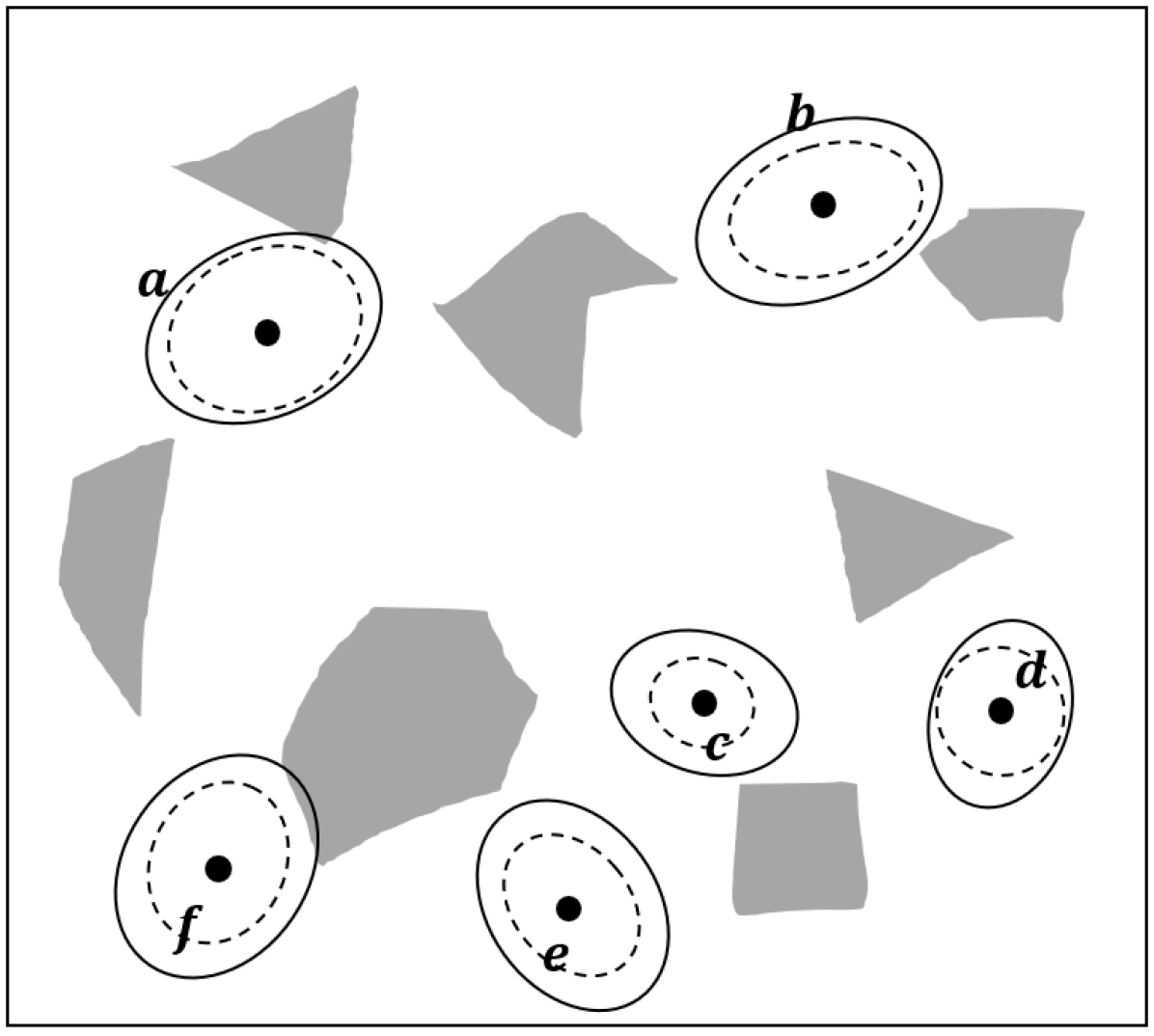
An illustration of the steps for building the CS-BRM is shown in Fig. 1.
The algorithm for constructing the CS-BRM is given in Algorithm 2.
The following procedures are used in the algorithm.
Sample Nodes: The function SampleNodes samples CS-BRM nodes.
A node in the CS-BRM is represented by the tuple , where is the state mean, is the prior estimated state covariance, and is the prior state estimation error covariance.
Since , the node can also be equivalently represented by . Note that we can compute the a posteriori convariances and using and .
For constructing node , the algorithm starts by sampling the free state space, which provides the mean of the distribution.
Then, an estimated state covariance is sampled from the space of symmetric and positive definite matrix space.
Similarly, a state estimation error covariance is also sampled at node .
is the initial condition of the Kalman filter update for the edges that are coming out of node .
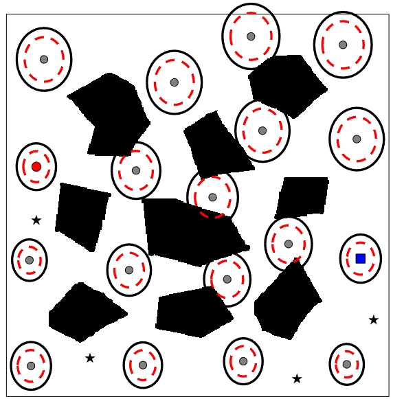
In Fig. 1(a), for each node, is shown as a black dot, is shown as a solid ellipse, and is shown as a dashed ellipse.
Neighbor: The function Neighbor finds all the nodes in that are within a given distance to node , where is a node set containing all nodes in the CS-BRM.
Mean Trajectory: Given two nodes and , MTraj uses the mean controller (18) and Algorithm 1 to find the compatible nominal trajectory, which is also the mean trajectory from to .
The function returns the mean control , mean trajectory , and the cost of the mean control .
Obstacle Checking: The function ObstacleFree returns true if the mean trajectory is collision free.
Kalman Filter: Given two nodes and , KF returns the prior estimation error covariance at the last time step of the trajectory from to .
Covariance Control: CovControl solves the covariance control problem from to .
It returns the control and the cost .
Monte Carlo: We use Monte Carlo simulations to calculate the probability of collision of the edges.
For edge , the initial state and initial state estimate are sampled from their corresponding distributions.
The state trajectory is simulated using the mean control and covariance control .
Then, collision checking is performed on the simulated state trajectory.
By repeating this process, we approximate the probability of collision of this edge.
In our implementation the collision cost is taken to be proportional to the probability of collision along that edge.
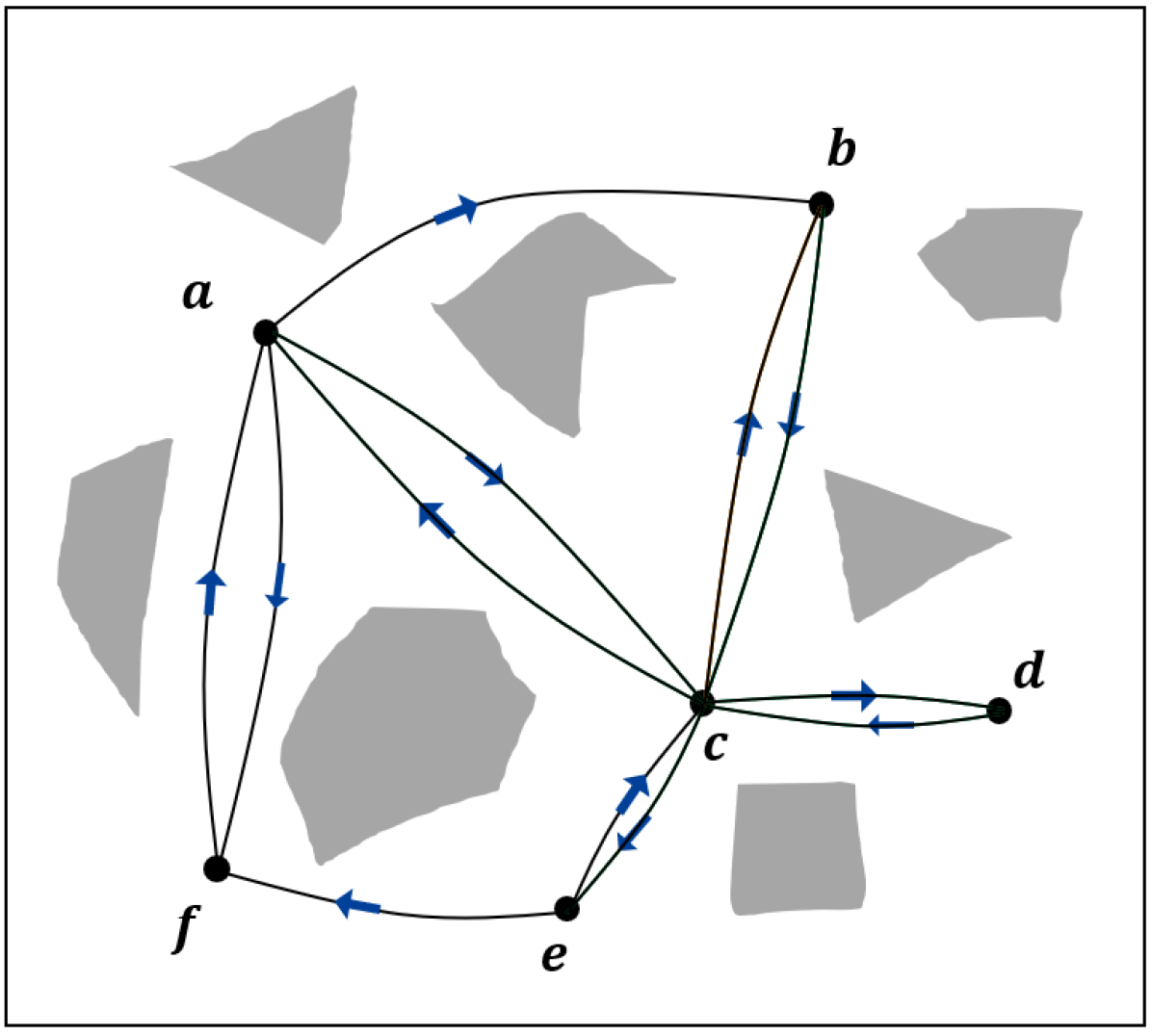
Algorithm 2 starts by sampling nodes in the belief space using SampleNodes (Line 1). Lines 3-17 are the steps to add CS-BRM edges. Given two neighboring nodes and , Lines 6-13 try to construct the edge and Lines 14-16 try to construct the edge .
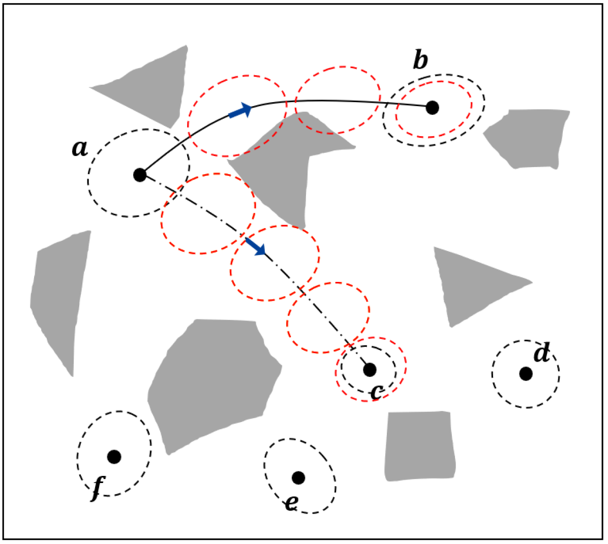
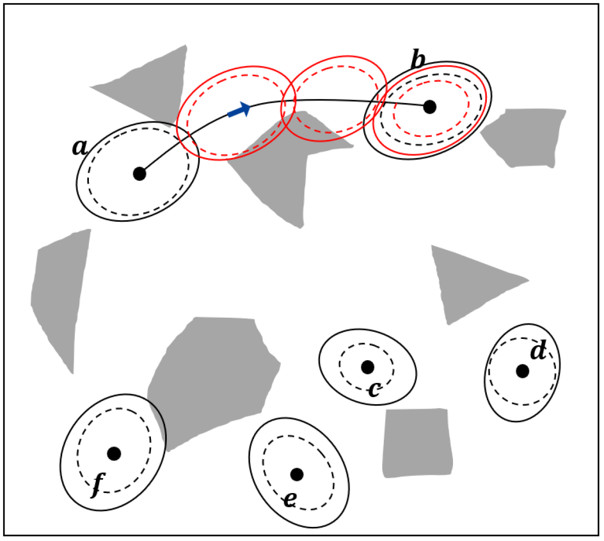
Every edge in the CS-BRM is constructed by solving a covariance steering problem. Each node tries to connect to its neighboring nodes if possible. First, for each edge, we use Algorithm 1 to find the mean trajectory of that edge (Line 6). Next, we check if the mean trajectory is collision-free. Only if the mean trajectory is collision-free do we proceed to the next step of edge construction. Then, the Kalman filter updates are simulated, which give the state estimation error covariance at every time step along that edge. The state estimation error covariances of the edges and are shown as red dash ellipses in Figure 1(c). Take the edge as an example. The initial condition of the Kalman filter is . The prior estimation error covariance at the final time-step, , is compared with the state estimation error covariance of node , . If (Line 9), the algorithm proceeds to solve the covariance control problem and this edge is added to the graph. For the covariance control problem of edge , the initial constraint and the terminal constraint are given by and . The covariance is computed using and . The final edge controller is the combination of the mean controller, covariance controller, and the Kalman filter.
In addition to the edge controller, the edge cost is computed for each edge. The edge cost is a weighted sum of , , and . With covariance steering serving as the lower-level controller, the higher-level motion planning problem using the roadmap is a graph search problem similarly to a PRM. Thus, the covariance steering approach transforms the belief space roadmap into traditional PRM with specific edge costs.
In CS-BRM, each edge is an independent covariance steering problem and the planned path using CS-BRM consists of a concatenation of edges. Since the terminal estimated state covariance satisfies an inequality constraint (17) and the terminal state estimation error covariance satisfies an inequality relation by construction (Line 9), it is important to verify that the covariance constraints at all nodes are still satisfied by concatenating the edges.
To this end, consider the covariance steering problem from node to node . For the edge , we have the initial constraints , , and the terminal covariance constraint . Note that the constraint is satisfied for (Line 9, Algorithm 2). Suppose that the solution of the covariance control problem of edge is the feedback gain . By concatenating the edges, the system may not start exactly at node . Instead, it will start at some node that satisfies and . Next, we show that by applying the pre-computed feedback gain , the terminal covariance still satisfies for the new covariances and . Before verifying this result, we provide a property of the covariance of the Kalman filter. Given an initial estimation error covariance , we obtain a sequence of error covariances using the Kalman filter updates (7). Similarly, given the new initial error covariance which satisfies , we obtain a new sequence of error covariances . We have the following lemma.
Lemma 1
If , then , for all .
The proof of this lemma is omitted. A proof of a similar result can be found in [18]. From Lemma 1, it is straightforward to show that, if , we also have for all .
Proposition 2
Consider a path on the CS-BRM roadmap, where the initial node of the path is denoted by and the final node of the path is denoted by . Starting from the initial node and following this path by applying the sequence of edge controllers, the robot will arrive at a belief node such that , , and .
The proof of this proposition is straightforward and is omitted. Proposition 2 guarantees that, when planning on the CS-BRM roadmap, the covariance at each arrived node is always smaller than the assigned fixed covariance at the corresponding node of the CS-BRM roadmap.
VI Numerical Examples
In this section, we first illustrate our theoretical results for the motion planning problem of a 2-D double integrator. We compare our method with the SLQG-FIRM algorithm [14], and we show that our method overcomes some of the limitations of SLQG-FIRM. Subsequently, the problem of a fixed-wing aerial vehicle in a 3-D environment is studied.
VI-A 2-D Double Integrator
A 2-D double integrator is a linear system with a 4-dimensional state space given by its position and velocity, and a 2-dimensional control space given by its acceleration.
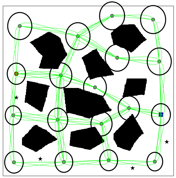
The environment considered is shown in Figure 2. There are landmarks placed in the environment, which are represented by black stars. The black polygonal shapes represent the obstacles. The agent observes all landmarks and obtains estimates of its position at all time steps. The agent achieves better position estimates when it is closer to the landmarks. Let the Euclidean distance between the position of the 2-D double integrator and the landmarks be given by . Then, the position measurement corresponding to landmark is
| (24) |
where is a parameter related to the intensity of the position measurement noise that is set to , and is a two-dimensional standard Gaussian random vector. The velocity measurement is given by
| (25) |
where is a parameter related to the intensity of the velocity measurement noise that is set to , and is a two-dimensional standard Gaussian random vector. Thus, the total measurement vector is a dimensional vector, composed of position measurements and one velocity measurement.
The sampled CS-BRM nodes are shown in Figure 2(a). The velocities are restricted to be zero for the purpose of comparison with SLQG-FIRM. The gray dots are the state means of the nodes. The red dot shows the position of the starting node and the blue square shows the position of the goal node. The black ellipses around the state represent the confidence intervals of the position covariances. The red dash ellipses correspond to the prior estimation error covariances. Following Algorithm 2, the edge controllers are computed using the covariance steering controller for each edge and the collision cost is computed using Monte Carlo simulations. The final CS-BRM is given in Figure 2(b).
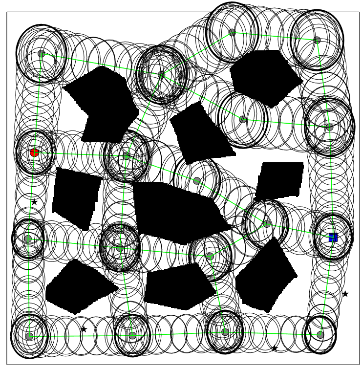
After the CS-BRM is built, the path planning problem on CS-BRM is the same as the problem of planning using a PRM, which can be easily solved using a graph search algorithm. The difference between the CS-BRM and PRM is that the edge cost in CS-BRM is specifically designed to deal with dynamical system models and uncertainties, and the transition between two nodes of CS-BRM is achieved using covariance steering as the edge controller.
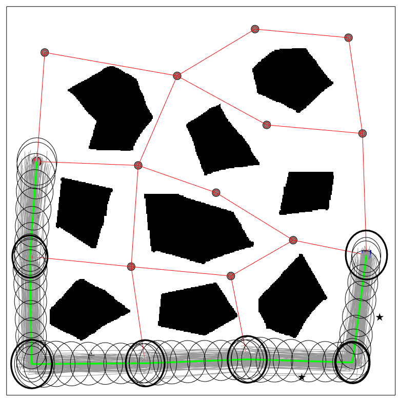
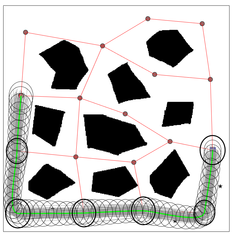
The planning results of CS-BRM and SLQG-FIRM are given in Figure 3. The paths goes through the same set of belief nodes for this example. In Figure 3(b), the red ellipses are the state covariances at the last step of the time-varying LQG controller. As we see, each one of the ellipses is larger than the corresponding state covariance of the intermediate belief node (bold black ellipses). Thus, a converging step is required at every intermediate node. The time-varying LQG controller is switched to the SLQG controller until the state covariance converges to a value that is smaller than the state covariance of the belief nodes (bold black ellipses).
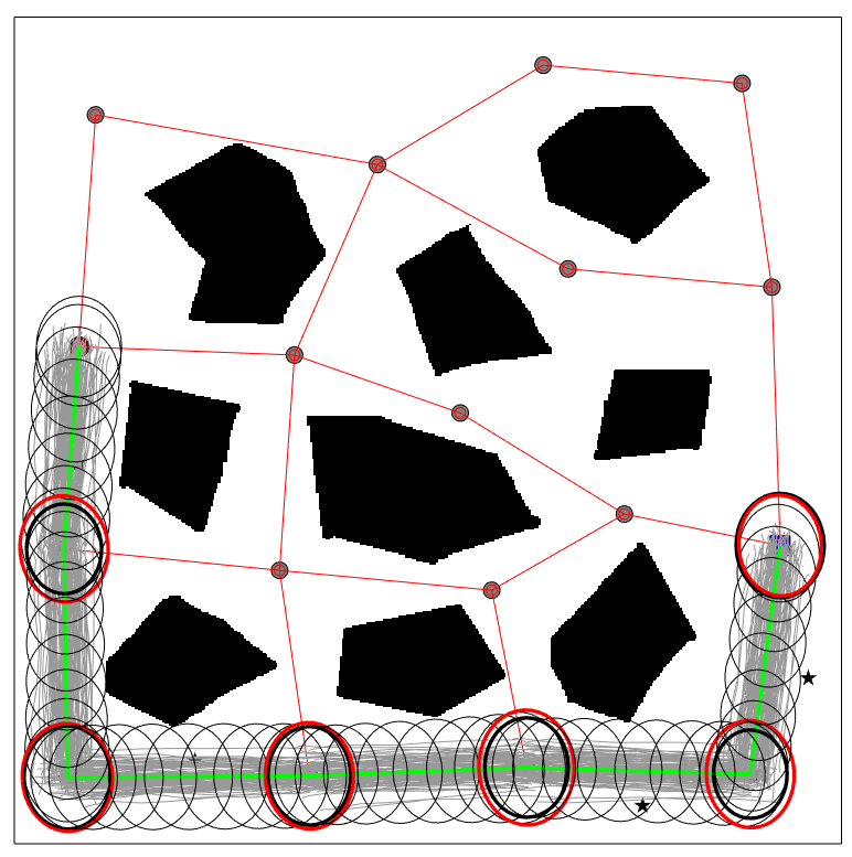
The CS-BRM that samples nonstationary nodes is shown in Figure 4(a). For clarity, only the mean trajectories of the edges are shown (green lines). The environment, the sampled mean positions, and the sampled covariances are all the same as those in Figure 3(a) and 3(b). The only difference is that multiple velocities are sampled at each position in Figure 4(a). The planned path is shown in Figure 4(b). The cost of the planned path is , which is much lower than the cost of the paths in Figure 3(a) and Figure 3(b), which are and respectively. The decrease in the path cost is due to the decrease of the mean control cost. In Figure 3(b), the robot has to stop (zero velocity) at every intermediate node. With the proposed method, the robot goes through each intermediate node smoothly, which results in a more efficient path.
VI-B Fixed-Wing Aircraft
In this section, we apply the proposed method on a nonlinear example, namely, planning for a fixed-wing aerial vehicle [32]. The discrete-time system model is given by
| (26) |
where the 4-dimensional state space is given by , where is the 3-D position of the vehicle, and is the heading angle. The 3-D control input space is given by , where is the air speed, is the flight-path angle, and is the bank angle, is the time step size, , , are standard Gaussian random variables, , , , and are multipliers correspond to the magnitude of the noise. Their values are all set to be .
Similar to the 2-D double integrator example, several landmarks are placed in the environment. Let the Euclidean distance between the 3D position of the vehicle and the landmarks be given by . Then, the position measurement corresponding to landmark is
| (27) |
where is a parameter related to the intensity of the noise of the measurement and is set to , and is a 4-dimensional standard Gaussian random vector. Thus, the total measurement vector is a -dimensional vector, where is the number of landmarks.
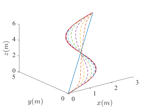
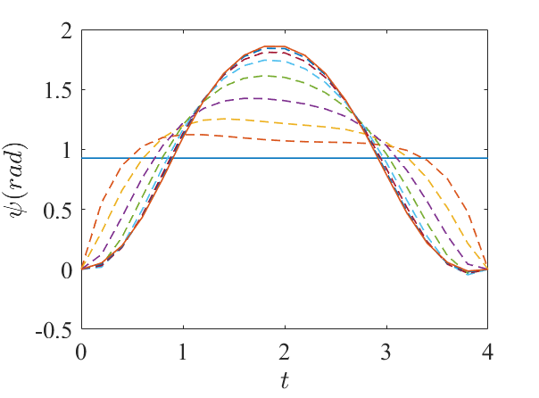
Algorithm 1 was used to find a compatible nominal trajectory for the fixed-wing vehicle. One example is given in Figure 5. The nominal trajectory and the reference trajectory are initialized as straight lines in all four state dimensions and the three control input dimensions. The algorithm converged in eight iterations.
The planning environment is shown in Figure 6. The four spheres in the middle of the environment are the obstacles. The three black stars represent the landmarks. The black circles represent the state mean (position) of the nodes. The red dot shows the position of the starting node and the blue square shows the position of the goal node. The state means are deterministically chosen to discretize the environment. The covariances of the nodes are not showed.
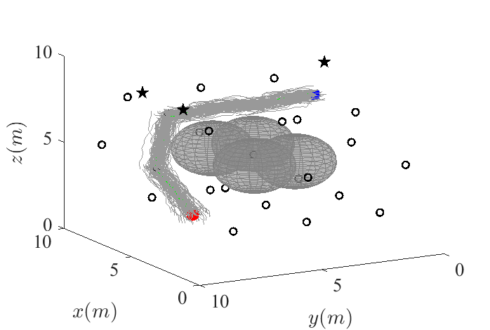
The planned path using this CS-BRM is also shown in Figure 6. Similarly to the example in Section VI-A, instead of flying through the narrow passage between the four obstacles, which resulting a high probability of collision, the algorithm choose a path that trades off between control cost and collision cost while minimizing the total edge costs.
VII Conclusion
A belief space roadmap (BRM) algorithm is developed in this paper. The nodes in BRM represent distributions of the state of the system and are sampled in the belief space. The main idea is to use covariance steering to design the edge controllers of the BRM graph to steer the system from one distribution to another. Compared to [14], the proposed method allows sampling nonstationary belief nodes, which has the advantage of more complete exploration of the belief space. For covariance steering of nonlinear systems, we introduce the concept of compatible nominal trajectories, which aim to better approximate the nonlinear dynamics through successive linearization. We also propose an efficient algorithm to compute compatible nominal trajectories. Compared to the standard PRM, the additional computation load comes from the computation of the edge controllers and edge cost evaluations, which, however, are done offline. By explicitly incorporating motion and observation uncertainties, we show that the proposed CS-BRM algorithm generates efficient motion plans that take into account both the control effort and collision probability.
Acknowledgments
This work has been supported by NSF awards IIS-1617630 and IIS-2008695, NASA NSTRF Fellowship 80NSSC17K0093, and ARL under CRA DCIST W911NF-17-2-0181. The authors would also like to thank Dipankar Maity for many insightful discussions regarding the output-feedback covariance steering problem.
References
- [1] B. Bonet and H. Geffner, “Planning with incomplete information as heuristic search in belief space,” in International Conference on Artificial Intelligence Planning Systems, Breckenridge, CO, April 2000, pp. 52–61.
- [2] S. Thrun, W. Burgard, and D. Fox, Probabilistic Robotics. MIT Press, 2005.
- [3] J. Van Den Berg, S. Patil, and R. Alterovitz, “Motion planning under uncertainty using iterative local optimization in belief space,” The International Journal of Robotics Research, vol. 31, no. 11, pp. 1263–1278, 2012.
- [4] L. P. Kaelbling, M. L. Littman, and A. R. Cassandra, “Planning and acting in partially observable stochastic domains,” Artificial Intelligence, vol. 101, pp. 99–134, 1998.
- [5] S. C. Ong, S. W. Png, D. Hsu, and W. S. Lee, “Planning under uncertainty for robotic tasks with mixed observability,” The International Journal of Robotics Research, vol. 29, no. 8, pp. 1053–1068, 2010.
- [6] S. Ross, J. Pineau, S. Paquet, and B. Chaib-Draa, “Online planning algorithms for POMDP,” Journal of Artificial Intelligence Research, vol. 32, pp. 663–704, 2008.
- [7] G. Shani, J. Pineau, and R. Kaplow, “A survey of point-based POMDP solvers,” Autonomous Agents and Multi-Agent Systems, vol. 27, no. 1, pp. 1–51, 2013.
- [8] A. Somani, N. Ye, D. Hsu, and W. S. Lee, “DESPOT: online POMDP planning with regularization,” Advances in neural information processing systems, vol. 26, pp. 1772–1780, 2013.
- [9] K. Sun, B. Schlotfeldt, G. J. Pappas, and V. Kumar, “Stochastic motion planning under partial observability for mobile robots with continuous range measurements,” IEEE Transactions on Robotics, 2020, early access.
- [10] R. Alterovitz, T. Siméon, and K. Y. Goldberg, “The stochastic motion roadmap: A sampling framework for planning with Markov motion uncertainty.” in Robotics: Science and systems, 2007, pp. 233–241.
- [11] S. Prentice and N. Roy, “The belief roadmap: Efficient planning in belief space by factoring the covariance,” The International Journal of Robotics Research, vol. 28, pp. 1448–1465, 2009.
- [12] L. E. Kavraki, P. Svestka, J. C. Latombe, and M. H. Overmars, “Probabilistic roadmaps for path planning in high-dimensional configuration spaces,” IEEE Transactions on Robotics and Automation, vol. 12, no. 4, pp. 566–580, 1996.
- [13] S. Karaman and E. Frazzoli, “Sampling-based algorithms for optimal motion planning,” The International Journal of Robotics Research, vol. 30, no. 7, pp. 846–894, June 2011.
- [14] A. A. Agha-Mohammadi, S. Chakravorty, and N. M. Amato, “FIRM: sampling-based feedback motion-planning under motion uncertainty and imperfect measurements,” The International Journal of Robotics Research, vol. 33, no. 2, pp. 268–304, 2014.
- [15] J. Van Den Berg, P. Abbeel, and K. Goldberg, “LQG-MP: optimized path planning for robots with motion uncertainty and imperfect state information,” The International Journal of Robotics Research, vol. 30, no. 7, pp. 895–913, 2011.
- [16] J. Pineau, G. Gordon, and S. Thrun, “Point-based value iteration: An anytime algorithm for POMDPs,” in International joint conference on artificial intelligence, vol. 3, Acapulco, Mexico, August 2003, pp. 1025–1032.
- [17] S. D. Bopardikar, B. Englot, A. Speranzon, and J. van den Berg, “Robust belief space planning under intermittent sensing via a maximum eigenvalue-based bound,” The International Journal of Robotics Research, vol. 35, no. 13, pp. 1609–1626, 2016.
- [18] A. Bry and N. Roy, “Rapidly-exploring random belief trees for motion planning under uncertainty,” in 2011 IEEE international conference on robotics and automation. IEEE, 2011, pp. 723–730.
- [19] A. A. Agha-Mohammadi, S. Chakravorty, and N. M. Amato, “Periodic feedback motion planning in belief space for non-holonomic and/or nonstoppable robots,” Technical Report: TR12-003, Parasol Lab., CSE Dept., Texas A&M University, pp. 1–23, 2012.
- [20] A. A. Agha-mohammadi, S. Agarwal, S. K. Kim, S. Chakravorty, and N. M. Amato, “SLAP: simultaneous localization and planning under uncertainty via dynamic replanning in belief space,” IEEE Transactions on Robotics, vol. 34, no. 5, pp. 1195–1214, 2018.
- [21] Y. Chen, T. T. Georgiou, and M. Pavon, “Optimal steering of a linear stochastic system to a final probability distribution, Part I,” IEEE Transactions on Automatic Control, vol. 61, p. 1158–1169, 2015.
- [22] ——, “Optimal steering of a linear stochastic system to a final probability distribution, part ii,” IEEE Transactions on Automatic Control, vol. 61, no. 5, pp. 1170–1180, 2015.
- [23] E. Bakolas, “Optimal covariance control for discrete-time stochastic linear systems subject to constraints,” in IEEE Conference on Decision and Control, Las Vegas, NV, December 2016, pp. 1153–1158.
- [24] M. Goldshtein and P. Tsiotras, “Finite-horizon covariance control of linear time-varying systems,” in IEEE Conference on Decision and Control, Melbourne, Australia, December 2017, p. 3606–3611.
- [25] K. Okamoto, M. Goldshtein, and P. Tsiotras, “Optimal covariance control for stochastic systems under chance constraints,” IEEE Control Systems Letters, vol. 2, no. 2, pp. 266–271, 2018.
- [26] J. Ridderhof, K. Okamoto, and P. Tsiotras, “Nonlinear uncertainty control with iterative covariance steering,” in IEEE Conference on Decision and Control, Nice, France, December 2019, pp. 3484–3490.
- [27] ——, “Chance constrained covariance control for linear stochastic systems with output feedback,” in IEEE Conference on Decision and Control, Jeju Island, South Korea, Dec. 8–11 2020, pp. 1153–1158.
- [28] Y. Chen, T. Georgiou, and M. Pavon, “Steering state statistics with output feedback,” in IEEE Conference on Decision and Control, Osaka, Japan, December 2015, pp. 6502–6507.
- [29] E. Bakolas, “Covariance control for discrete-time stochastic linear systems with incomplete state information,” in American Control Conference, Seattle, WA, May 2017, pp. 432–437.
- [30] J. T. Betts, “Survey of numerical methods for trajectory optimization,” Journal of Guidance, Control, and Dynamics, vol. 21, no. 2, pp. 193–207, 1998.
- [31] A. E. Bryson and Y. C. Ho, Applied Optimal Control: Optimization, Estimation and Control. CRC Press, 1975.
- [32] M. Owen, R. Beard, and T. McLain, “Implementing Dubins airplane paths on fixed-wing UAVs,” in Handbook of Unmanned Aerial Vehicles, K. Valavanis and G. Vachtsevanos, Eds. Springer, 2015, ch. 64, pp. 1677–1701.