BEAUTY Powered BEAST
Abstract
We study distribution-free goodness-of-fit tests with the proposed Binary Expansion Approximation of UniformiTY (BEAUTY) approach. This method generalizes the renowned Euler’s formula, and approximates the characteristic function of any copula through a linear combination of expectations of binary interactions from marginal binary expansions. This novel theory enables a unification of many important tests of independence via approximations from specific quadratic forms of symmetry statistics, where the deterministic weight matrix characterizes the power properties of each test. To achieve a robust power, we examine test statistics with data-adaptive weights, referred to as the Binary Expansion Adaptive Symmetry Test (BEAST). For any given alternative, we demonstrate that the Neyman-Pearson test can be approximated by an oracle weighted sum of symmetry statistics. The BEAST with this oracle provides a useful benchmark of feasible power. To approach this oracle power, we devise the BEAST through a regularized resampling approximation of the oracle test. The BEAST improves the empirical power of many existing tests against a wide spectrum of common alternatives and delivers a clear interpretation of dependency forms when significant.
Keywords— Nonparametric Inference; Goodness-of-fit Test; Test of Independence; Resampling; Characteristic Function; Euler’s Formula
1 Introduction
As we enter the era of data dominance, the prevalence of complex datasets presents significant challenges to traditional parametric inference methods, which often lose efficacy in practical applications, as flawless models are rarely attainable through scientific theories alone. In contrast, nonparametric methods deliver more robust inference, rendering them increasingly appealing for practical use. Hypotheses addressing particular structures of distributions are classified as goodness-of-fit tests (Lehmann and Romano, 2006). Notable progress within this domain is extensively documented in the literature, as exemplified by moment or cumulant based methods (Anderson and Darling, 1954; Stephens, 1976), likelihood ratio based methods (Cressie and Read, 1984; Fan and Huang, 2001; Zhang, 2002), empirical process based methods (Genest et al., 2006; Escanciano, 2006; Jager and Wellner, 2007; Genest et al., 2009; Kaiser and Soumendra, 2012), kernel based methods (González-Manteiga and Crujeiras, 2013; Sen and Sen, 2014), and randomization based methods (Janková et al., 2020; Kim and Ramdas, 2020; Barber and Janson, 2022), along with the references cited therein.
Without loss of generality, we consider a -dimensional distribution in for notation convenience. Let denote a -dimensional vector whose marginal distributions are continuous and whose joint distribution has a support within . With the above notation, the goodness-of-fit test for some hypothesized distribution can be written as follows:
| (1.1) |
for some distance between distributions and some Some common choices of include the total variation (TV) distance (Zhang, 2019) and the distance (Berrett et al., 2021).
Two important special cases of goodness-of-fit tests are the test of uniformity and the test of independence. The test of uniformity can be formulated as
| (1.2) |
where denotes the uniform distribution. The test of independence can be formulated as
| (1.3) |
where and are and dimensional random vectors with distributions and respectively. Applications of the test of uniformity include Diaz Rivero and Dvorkin (2020); Liang et al. (2001). Important developments in distribution-free tests of independence include cumulative distribution function (CDF) based methods (Hoeffding, 1948; Blum et al., 1961; Genest and Verret, 2005; Kojadinovic and Holmes, 2009; Genest et al., 2019; Chatterjee, 2020; Cao and Bickel, 2020), kernel based methods (Székely et al., 2007; Gretton et al., 2007; Zheng et al., 2012; Sejdinovic et al., 2014; Pfister et al., 2016; Zhu et al., 2017; Jin and Matteson, 2018; Balakrishnan and Wasserman, 2019a; Shi et al., 2020; Deb et al., 2020; Geenens and de Micheaux, 2020; Berrett et al., 2021; Berrett and Samworth, 2021), binning based methods (Miller and Siegmund, 1982; Reshef et al., 2011; Heller et al., 2013; Kinney and Atwal, 2014; Heller et al., 2016; Heller and Heller, 2016; Ma and Mao, 2019; Lee et al., 2023), and references therein.
To facilitate the analysis of large datasets, some desirable attributes of distribution-free tests of independence include (a) a robust high power against a wide range of alternatives, (b) a clear interpretation of the form of dependency upon rejection, and (c) a computationally efficient algorithm. An example of recent development towards these goals is the binary expansion testing (BET) framework and the Max BET procedure in Zhang (2019). It was shown that the Max BET is minimax optimal in power under mild conditions, has clear interpretability of statistical significance and is implemented through computationally efficient bitwise operations Zhao et al. (2023b). Potential improvements of the Max BET include the followings: (a) The procedure is only univariate and needs to be generalized to higher dimensions. (b) The multiplicity correction is through the conservative Bonferrnoni procedure, which leaves room for further enhancement of power. In Lee et al. (2023), random projections are applied to the multivariate observations to reduce the dimension to one, so that the univariate methods of Zhang (2019) are applicable. An ensembled approach involving distance correlation is further used to improve the power towards monotone relationships.
In this paper, we develop an in-depth understanding of the BET framework and construct a class of powerful distribution-free goodness-of-fit tests, encompassing both the uniformity test and the independence test between a random vector and a random variable. While many tests have been devised for this problem, Zhang (2019) showed that uniform consistency for testing (1.3) is generally unachievable for all alternative distributions. Analogous results for the -distance was recently documented by Berrett et al. (2021). These results reaffirm earlier observations by LeCam (1973); Barron (1989); Balakrishnan and Wasserman (2019b).
Practically, this finding indicates that each test encounters a “blind spot,” resulting in a significant loss of power. To mitigate the power loss arising from non-uniform consistency, Zhang (2019) introduced the binary expansion statistics (BEStat) framework to restrict the space of alternative distributions up to a suitable finite resolution. The BEStat approach is inspired by the classical probability result of the binary expansion of a uniformly distributed random variable (Kac, 1959), as stated below.
Theorem 1.1.
If then where , that is with equal probabilities.
Theorem 1.1 allows the approximation of the -field generated by using for any positive integer depth . This filtration approach for testing uniformity facilitates a universal distribution approximation, an identifiable model, and uniformly consistent tests at any depth . The testing framework based on the binary expansion filtration approximation is referred to as the binary expansion testing (BET). Specifically, the BET of approximate uniformity for is
| (1.4) |
where is the uniform distribution over -dimensional dyadic rationals
1.1 Our Contributions
Our study of the BET framework is inspired by the celebrated Euler’s formula,
which is often regarded as one of the most beautiful equations in mathematics. In particular, when , one has Euler’s identity, , which connects the five most important numbers in mathematics in one simple yet deep equation. Beside the beauty of this equation, how is it useful for statisticians? To see that, consider any binary variable (not necessarily symmetric) which takes values or . Through the parity of the sine and cosine functions, one can easily show the following binary Euler’s equation. Since we were not aware of any reference of this equation in literature, we formally state it below.
Lemma 1.2 (Binary Euler’s Equation).
For any binary random variable with possible outcomes of or , it holds that for any
| (1.5) |
Lemma 1.2 generalizes Euler’s formula with additional randomness from a binary variable and reduces its complex exponentiation to its linear polynomial. To the best of our knowledge, no other random variables enjoy the same remarkable attribute. Moreover, note that the random variable in (1.5) is closely related to characteristic functions, particularly when it is combined with the binary expansion in Theorem 1.1. For example, for and for any we have
| (1.6) |
The complex exponent of can be approximated by a polynomial of the binary variables in its binary expansion! Moreover, we show in Section 2 that this approximation is universal for any -dimensional vector supported within . We refer this universal binary interaction approximation of the complex exponent and the characteristic function as the Binary Expansion Approximation of UniformiTY (BEAUTY) in Theorem 2.2.
Based on the BEAUTY, in this paper we make the following three main novel contributions to the problem of nonparametric tests of independence:
1. A unification of important nonparamatric tests of independence. In Section 3, we show that many important tests of independence in literature can be approximated by some quadratic forms of symmetry statistics, which are shown to be complete sufficient statistics for dependence in Zhang (2019). In particular, each of these test statistics corresponds to a different deterministic weight matrix in the quadratic form, which in turn dictates the power properties of the test. Therefore, this deterministic weight in existing test statistics creates the key issue on uniformity and robustness of the test, as it may favor certain alternatives but cause a substantial loss of power for other alternatives. Following this observation, we consider a test statistic that has data-adaptive weights to make automatic adjustments under different situations so as to achieve a robust power. We refer this test as the Binary Expansion Adaptive Symmetry Test (BEAST), as described in Section 4.
2. A benchmark of feasible power from the BEAST with oracle. We begin by considering the test of uniformity. By utilizing the properties of the binary expansion filtration, we show in a heuristic asymptotic study of the BEAST a surprising fact that for any given alternative, the Neyman-Pearson test for testing uniformity can be approximated by a weighted sum of symmetry statistics. We thus develop the BEAST through an oracle approach over this Neyman-Pearson one-dimensional projection of symmetry statistics, which quantifies a boundary of feasible power performance. Numerical studies in Section 5 show that the BEAST with oracle leads a wide range of prevailing tests by a surprisingly huge margin under all alternatives we considered. This enormous margin thus provides helpful information about the potential of substantial power improvement for each alternative. To the best of our knowledge, there is no other type of similar approach or results to study the potential performance of a test of uniformity or independence. Therefore, the BEAST with oracle sets a novel and useful benchmark for the feasible power under any alternative. Moreover, it provides guidance for choosing suitable weights to boost the power of the test.
3. A powerful and robust BEAST from a regularized resampling approximation of the oracle. Motivated by the form of the BEAST with oracle, we construct the practical BEAST to approximate the optimal power by approximating the oracle weights in testing uniformity. The proposed BEAST combines the ideas of resampling and regularization to obtain data-adaptive weights that adjusts the statistic towards the oracle under each alternative. Here resampling helps the approximation of the sampling distribution of the oracle test statistic, and regularization screens the noise in the estimation of optimal weights. This test is applied to the problem to the test of independence. Simulation studies in Section 5 demonstrate that the BEAST improves the power of many existing tests of univariate or multivariate independence against many common forms of non-uniformity, particularly multimodal and nonlinear ones. Besides its robust power, the BEAST provides clear and meaningful interpretations of statistical significance, which we demonstrate in Section 6. We conclude our paper with discussions in Section 7. Details of notation, theoretical proofs and additional numerical results are deferred to Supplementary materials.
2 The BEAUTY Equation
To further understand the BET framework, we first develop the general binary expansion for any random vector supported within as in Lemma 2.1.
Lemma 2.1.
Let be a random vector supported within . There exists a sequence of random variables , , , which only take values and , such that uniformly as , where
A classical construction of ’s is to consider the binary numeral system representation of real numbers, or data bits (Kac, 1959; Zhang, 2019). We refer the collection of variables as the general binary expansion of and denote as the depth- binary approximation of . Let denote the set of all binary matrices with entries being either or . We use a matrix to index an interaction of binary variables via . For the zero matrix we define
With the above notation, we develop the following theorem on the binary expansion approximation of uniformity (BEAUTY), which provides an approximation of the characteristic function of any distribution supported within from the expectation of a polynomial of general binary expansion interactions.
Theorem 2.2 (Binary Expansion Approximation of Uniformity, BEAUTY).
Let be a -dimensional random vector such that . Let be the characteristic function of for any . We have
| (2.1) |
and
| (2.2) |
where
Building upon Lemma 1.2, (2.1) equates a complex exponent and a polynomial of binary variable ’s derived from the binary expansion of . Equation (2.2) reveals that the characteristic function of any random vector supported within can be approximated by a linear combination of ’s, representing products of homogeneous trigonometric functions. As per Theorem 1.3 in Zhao et al. (2023a), these functions are linearly independent. Furthermore, the coefficients of this linear combination correspond to the expectations of all binary variables in the -field induced by . These expectations encapsulate the distributional properties of , and inference on them yields crucial insights into the distribution of . Specifically, they provide clear insights about the goodness-of-fit tests by translating distributional properties into those of ’s. Moreover, sufficient statistics for ’s are the symmetry statistics and equivalently Consequently, test statistics should be constructed as a function of ’s. We list some important examples connecting goodness-of-fit tests and ’s below:
(1) Test of uniformity. Consider the collection of non-zero ’s, . Note that if and only if for where is any positive integer. Consequently,
i.e., (2.2) recovers the characteristic function of Unif Therefore, the test of approximate uniformity (1.4) is equivalent to test for any positive integer ,
(2) Test of independence between two univariate random variables. The BEAUTY equation in Theorem 2.2 offers clear insights into the test of independence for bivariate copula up to a certain depth . When , it is always possible to transform and into uniform random variables on using their marginal distributions. In this context, Zhang (2019) demonstrated that test (1.3) with considered the following test for any positive integer ,
where . Here, \raisebox{-.9pt} {r}⃝ denotes the row binding of matrices with the same number of columns (see Definition LABEL:def:_rbind in the supplement).
(3) Test of independence between response and predictors. The BEAUTY equation provides an in-depth understanding of testing the association between predictors and an arbitrary response , extending beyond the scope of traditional regressions. As noticed before, can always be transformed into a uniform variable on . Note that is independent of if and only if for any positive integer . Note also that from Theorem 1.3 in Zhao et al. (2023a), the ’s are linearly independent in the function space. Therefore, by comparing the characteristic function of the joint distribution and the product of marginal characteristic functions, we see that for any positive integer , the null hypothesis that and are independent is equivalent to the following hypothesis over the expectations of ’s: :
where .
(4) Test of independence between a uniform vector and an arbitrary vector. For random vector and arbitrary random vector within , by leveraging Theorem 2.2, the null hypothesis that posits the independence of and can be approximated by the following one over the expectations of ’s:
where .
3 Unification of Several Tests of Independence
To construct a powerful test statistic, we first study existing tests of independence and their properties under the BET framework. We consider three important test statistics: Spearman’s (Spearman, 1904), the statistics, and the distance correlation (Székely et al., 2007). We find that each of these statistics can be approximated by a certain quadratic form of symmetry statistics. We further discuss the effect of the weight matrix in the quadratic forms on their power properties.
Since each specific statistic may involve a different collection of binary interactions, we denote a collection of certain ’s by For such a collection , we denote the vector of ’s, ’s and ’s with by , and , respectively.
3.1 Spearman’s
As a robust version of the Pearson correlation, the Spearman’s statistic leads to a test with high asymptotic relative efficiency compared to the optimal test with Pearson correlation under bivariate normal distribution (Lehmann and Romano, 2006). We show below it can be approximated by a quadratic form of symmetry statistics.
When and are marginally uniformly distributed over , Spearman’s can be written as the correlation between and , i.e.,
| (3.1) |
where consists of matrices whose rows are both binary vectors with only one unique , and the -dimensional vector has entry corresponding to The test based on Spearman’s rejects the null when the estimate of has a large absolute value. This test statistic can be approximated with
which is a quadratic form with a rank-one weight matrix
Although the test based on Spearman’s has a higher power against the linear form of dependency particularly present in bivariate normal distributions, we see from and that this test only considers out of cross interactions of binary variables in . Thus this test is not capable of detecting complex nonlinear forms of dependency.
3.2 Test Statistic
When and are distributed, the binary expansion up to depth effectively leads to a discretization of into a contingency table. Classical tests for contingency tables such as -test can thus be applied. Similar tests include Fisher’s exact test and its extensions (Ma and Mao, 2019). Multivariate extensions of these methods include Gorsky and Ma (2018); Lee et al. (2023).
In Zhang (2019), it is shown that the -statistic at depth can be written as the sum of squares of symmetry statistics for cross interactions. Thus,
where is the collection of all cross interactions. The weight matrix for is thus the identity matrix .
The Max BET proposed in Zhang (2019) can be approximated by a quadratic form with another diagonal weight matrix, which we explain in the Supplementary Materials. These tests with diagonal weights can detect signals among the squared symmetry statistics, but might be powerless for signals from their cross products.
3.3 Distance Correlation between uniformly distributed random vectors
To study the dependency between a -dimensional vector and a -dimensional vector , in Székely et al. (2007), a class of measures of dependence is defined as
| (3.2) |
where is the characteristic function of the joint distribution of is a suitable weight function, and is the characteristic function of . Note that if and only if and are independent. The distance correlation is then defined through and admits some desirable properties such as universal consistency against alternatives with finite expectation.
When and , by Theorem 2.2, the term corresponding to cancels with , and we can write (3.2) as
| (3.3) |
where , and the weight matrix consists of constants ’s from the integration over and . The test is significant when the empirical quadratic form is large, where
Note that here depends only on the weight function and is deterministic. Hence, the test based on will have a high power when the vector of ’s from the alternative distribution lies in the subspace spanned by eigenvectors of corresponding to its largest eigenvalues. On the other hand, if instead the signals lie in the subspace spanned by eigenvectors of corresponding to its lowest eigenvalues, then the power of the test could be considerably compromised. Therefore, a deterministic weight over symmetry statistics becomes a general uniformity issue of existing test statistics. In the next section, we study data-adaptive weights with the aim to improve the power by setting proper weights both among diagonal and off-diagonal entries in the matrix.
4 The BEAST and Its Properties
4.1 The First Two Moments of Binary Interactions
The unification in Section 3 inspires us to consider a class of nonparametric statistics for the goodness-of-fit test as a weighted sum of symmetry statistics. Since the properties of this form of statistics are closely related to the first two moments of the binary interaction variables in the filtration, we consider the collection of all nontrivial binary interactions and study the moment properties of the corresponding binary random vector
We begin by studying the connection between the vector and the multinomial distribution from the corresponding discretization with categories. We order the indices ’s in by the integer corresponding to the binary vector representation where is the vectorization function. For example, the last (i.e. the th) entry in corresponds to the . We also denote the vector of cell probabilities in the multinomial distribution by Label the entries in by binary matrices through where each realization of the vector labels one of the intervals for dimension from low to high according to 1 plus the integer corresponding to the binary representation of . We define a random vector to denote one draw from the intervals from the discretization. With the above notation, we develop the general binary interaction design (BID) equation, which extends the two-dimensional case in Zhang (2019).
Theorem 4.1.
Let and Denote the Sylvester’s Hadamard matrix by We have the binary interaction design (BID) equation
| (4.1) |
In particular, we have the BID equation for the mean vector
| (4.2) |
and the corresponding BID equation for
| (4.3) |
where is the diagonal matrix with diagonal entries corresponding to .
The Hadamard matrix is also referred to as the Walsh matrix in engineering, where the linear transformation with is referred to as the Hadamard transform (Lynn, 1973; Golubov et al., 2012; Harmuth, 2013). The earliest referral to the Hadamard matrix we found in the statistical literature is Pearl (1971), and it is also closely related to the orthogonal full factorial design (Cox and Reid, 2000; Box et al., 2005). In our context of testing independence, the BID equation can be regarded as a transformation from the physical domain to the frequency domain, which turns the focus to global forms of non-uniformity instead of local ones. In developing statistics, this transformation facilitates regularizations through thresholding, as is equivalent to uniformity This transformation also enables clear interpretations of statistical significance with the form of dependency, as shown in Zhang (2019).
To study the power of the test of uniformity, we further study the properties of the first two moments of Let and denote the vector of expectations and the matrix of second moments of respectively. We summarize some properties of and in the following theorem.
Theorem 4.2.
We have the following results on the properties of first two moments of binary interaction variables in the binary expansion filtration.
-
(a)
The connection between the first and second moments of binary interactions:
(4.4) -
(b)
The connection between the harmonic mean of probabilities and the Hotelling’s quadratic form when :
(4.5) -
(c)
For with with constant
(4.6) -
(d)
Denote the vector-valued function by for each . As
(4.7)
To the best of our knowledge, the results in Theorem 4.2, despite their simplicity, have not been documented in literature. These simple results unveil interesting insights of the first two moments of binary variables in the filtration. The quadratic form in (4.4) characterizes the functional relationship between and . The two equations in (4.5) show that for binary variables, the Hotelling quadratic form is a monotone function of the harmonic mean of the cell probabilities in the corresponding multinomial distribution. The inequalities in (4.6) reveal the eigen structure of when the signal is weak. The Taylor expansion in (4.7) provides the asymptotic behavior of when the joint distribution is close to the uniform distribution. These insights shed important lights on how we can develop a powerful goodness-of-fit test, as we explain in Sections 4.2 and 4.3.
4.2 An Oracle Approach for Test Construction
In this section, we study how to construct a powerful robust nonparametric test of uniformity based on what we learned in Sections 3 and 4.1. As discussed in Section 3, the deterministic weights of symmetry statistics in existing tests create an issue on the uniformity and robustness: They make the test powerful for some alternatives but not for others. Therefore, we construct a test statistic with data-adaptive weights, which allow the test to adjust itself towards the alternative to improve the power. We refer this class of statistics as the binary expansion adaptive symmetry test (BEAST).
We construct our test through an oracle approach. Suppose we know from an oracle and thus as shown in Theorem 4.1. Note that by Theorem 4.1, 4.2 and 4.3 in Zhang (2019), under of (1.4), the distribution of is either pairwise independent centered binomial or uncorrelated centered hypergeometric, depending on whether the marginal distributions are known. Therefore, for fixed and , with a large and the central limit theorem on , we approximately have a simple-versus-simple hypothesis testing problem:
According to the fundamental Neyman-Pearson Lemma (Neyman and Pearson, 1933), the corresponding most powerful (MP) test is the likelihood ratio test. We thus consider the data-relevant part of the log-likelihood ratio of the above two distributions,
For a large , the dominating term in is By (4.7) in Theorem 4.2, the first order Taylor expansion of this term is precisely ! This implies that the MP test rejects when is colinear with The above heuristics thus suggests that we consider the oracle test statistic .
In our simulation studies in Section 5, since we know the form of the alternative distribution, we can estimate with high accuracy through an independent simulation. That is, with the known alternative distribution , for a large we simulate From the binary expansion of we obtain the vector of symmetry statistics and an estimate of denoted by The oracle test statistic from simulations is then
We show in simulations that even when is as small as , is powerful, and numerically it outperforms all existing competitors under consideration across a wide spectrum of alternatives and noise levels. For example, for the cases when the joint distributions are Gaussian with linear dependency, the power curves of dominate those of the distance correlation when and the F-test when which are known to be optimal. Compared to existing tests, the gain of the BEAST with oracle in power suggests that suitably chosen deterministic weights for the alternative provide a unified yet simple solution to improve the power. To the best of our knowledge, this is the first time that such a benchmark on the feasible power performance is available for the problem of testing uniformity.
Besides the useful insight about the feasible limit of power, the oracle also provides insights on the optimal weights under each alternative. For example, in simulations we find high colinearity between the approximate oracle weight vector and that of the Spearman’s , , as found in Section 3.1. This weight vector makes the one-sided test with more powerful than the two-sided test with Spearman’s
Although the optimal weight or is unknown in practice, an unbiased and asymptotically efficient estimate of is This motivates us to develop an approximation of through resampling and regularization, which we discuss next.
4.3 The BEAST Statistic
In practice, we are agnostic about Blindly replacing in with will result in colinearity with itself and the statistic reduces to the classical -test statistic. Traditionally, the data-splitting strategy has often been employed for this type of situations to facilitate data-driven decision (Hartigan, 1969; Cox, 1975), i.e., half of the data is used to calibrate the statistical procedure such as screening the null features (Wasserman and Roeder, 2009; Barber and Candès, 2019), determining the proper weights for individual hypotheses (Ignatiadis et al., 2016), recovering the optimal projection for dimension reducion (Huang, 2015), and estimating the latent loading for factor models (Fan et al., 2019), while a statistical decision is implemented using the remaining half. However, the single data-splitting procedure only uses half of the data for decision making, which inevitably bears undesirable randomness and therefore leads to power loss for hypothesis testing. Some recent efforts have shown that this shortcoming can be lessened by using multiple splittings (Romano and DiCiccio, 2019; Liu et al., 2019; Dai et al., 2020).
Motivated by the principle of multiple splitting, we propose to approximate through resampling: We replace in with , and we replace in with its resampling version . Important resampling methods include bootstrap (Efron and Tibshirani, 1994) and subsampling (Politis et al., 1999). Bootstrap and subampling are known to have similar performance in approximating the sampling distribution of the target statistic. In this paper, we use the subsampling method to facilitate the calculation of the empirical copula distribution when the marginal distributions are unknown Nelsen (2007). In addition to the above consideration, one intuition behind this resampling approach is to help distinguish the alternative distribution from the null: Under the null, since we expect the magnitude of and to be small and not very colinear after regularization. On the other hand, under the alternative, since we expect the two estimations of to be both colinear with and thus to be highly colinear themselves. Therefore, the magnitude of the test statistic could be different to help distinguish the alternative distribution from the null.
In addition, we apply regularization to accommodate sparsity, i.e., the non-uniformity can be explained by a few binary interactions ’s with This sparsity assumption is often reasonable in the BET framework, since is equivalent to the symmetry of distribution according to the interaction . Thus, sparsity over ’s is equivalent to a highly symmetric distribution. For example, if a multivariate distribution is symmetric in every direction, then each one-dimensional projection of this distribution has a real characteristic function. By Theorem 2.2, we have for all involving an even number of binary variables ( is even). Many global forms of dependency also correspond to sparse structures in
The estimation of under the sparsity assumption is closely related to the normal mean problem, where many good regularization based methods are readily available (Wasserman, 2006). For example, in Donoho and Johnstone (1994), it is shown that estimation with soft thresholding is nearly optimal. We denote the vector-valued soft thresholding function by for vector and threshold so that In construction of our test statistic, we choose to use soft-thresholding as a regularization step to screen the small observations in and due to the null distribution or due to the sparsity for certain interaction ’s under the alternative, thus improves the power of the test statistic.
In summary, we consider the approximation of through subsampling, while using regularization to obtain a good estimate of the optimal weight vector The detailed steps are listed below.
-
Step 1:
From observations of obtain subsamples of size : , For each subsample base on the binary expansions of , find the vector of average symmetry statistics .
-
Step 2:
Take the average over subsamples to obtain Apply the soft-thresholding function to get an estimate of as
-
Step 3:
The BEAST statistic is obtained as
(4.8)
We study the empirical power of the BEAST in Section 5, which shows that by approximating with regularization and subsampling, has a robust power against many alternative distributions, especially complex nonlinear forms of dependency.
We now study the asymptotic distributional properties of under the assumption of known marginal distributions. Denote the vector of cell proportions of the discretization out of samples by We have the following theorem on the distribution of the subsample symmetry statistic condition on .
Theorem 4.3.
Condition on as we have
where is the submatrix of with the first row and first column removed.
Theorem 4.3 holds both under the null distribution and the alternative distribution. This result thus provides useful guidance and efficient algorithms to simulate the null and alternative distributions of for any The detailed asymptotic distribution of with a positive and the analysis of the power function are useful for developing optimal adaptive tests and are interesting problems for future studies.
4.4 Practical Considerations
In this section, we discuss some practical considerations in applying the BEAST. The first practical issue is whether using the empirical CDF would lead to some loss of power. As discussed in Zhang (2019), the difference between using the known CDF and empirical CDF is similar to the difference between the multinomial model and the multivariate hypergeometric model for the contingency table, in which the theory and performance are similar too. In all of our numerical studies, we considered the method using the empirical CDF.
A related issue is the choice of depth and threshold in practice. In our simulations, we find that with , the BEAST with oracle has a higher power than the linear model based tests for Gaussian data, which indicates that is sufficiently large to detect many important forms of dependency. In our simulation studies in Section 5 below and Section D in the supplmentary materials, we also show the power is relatively stable as increases slightly. Moreover, data studies show that using can already provide many interesting findings Xiang et al. (2022) in practice. Therefore, we choose for this paper. We shall also choose a according to the large deviation of the symmetry statistic. That is approximately of these symmetry statistics under the null of uniformity will be thresholded to 0. A general optimal choice of and for some specific alternative should come from a trade-off between them and and the signal strength. This would be an interesting problem for future studies.
5 Simulation Studies
5.1 Testing Bivariate Independence
In this section, we consider the problem of testing the bivariate independence. The sample size is set to be . The BEAST with oracle and the BEAST are constructed with the empirical copula distribution and with , , , and . For the BEAST with oracle, we choose to obtain the oracle weights and for each alternative distribution, and the critical region is then obtained through draws from the bivariate uniform distribution over . For the BEAST, the critical region is formed with ’s permuted from the data. The level of all tests is set to be
We compare the power of the two versions of the BEAST with the following methods: the -test and its improvement the -statistic permutation (USP) test (Berrett et al., 2021; Berrett and Samworth, 2021) with the same discretization for , the Fisher exact scanning (Ma and Mao, 2019), the distance correlation (Székely et al., 2007), the -nearest neighbor mutual information (KNN-MI, Kinney and Atwal (2014)) with the default parameters, the -nearest neighbour based Mutual Information Test (MINT, Berrett and Samworth (2019)) with default averaging over , MaxBET (Zhang, 2019), BERET (Lee et al., 2023), and the high-dimensional multinomial test (HDMultinomial) by Balakrishnan and Wasserman (2019a). Among these tests, the HDMultinomial, the MINT, and the USP test are shown to be minimax optimal in power.
The data of the alternative distributions are generated according to the four different settings in Table 1 below. Parameter is evenly spaced over to represent the level of noise. The settings are chosen such that the power curves display a thorough comparison for different signal strengths. In Figure 1, simulations are conducted to calculate the empirical power of each test for each setting with a given .
| Scenario | Generation of | Generation of |
| Bivariate Normal | ||
| Parabolic | ||
| Circle | ||
| Checkerboard |
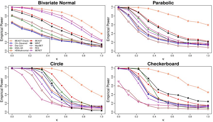
We first comment on the performance of the BEAST with oracle. Although this test is not achievable in practice, it provides many important insights in these simulation examples. From Figure 1, we see that with a small depth , the BEAST with oracle achieves the highest power among all methods, for every alternative distribution and every level of noise. In particular, under the bivariate normal case, the power curve of is higher than that of the distance correlation, while leaving substantial gaps to other nonparametric tests. The good performance of the distance correlation is expected, since it has been shown that it is a monotone function of Pearson correlation under normality (Székely et al., 2007). These facts thus again show that the BEAST with oracle can accurately approximate the optimal power under an alternative. Therefore, the BEAST with oracle provides a useful benchmark for the performance of tests.
Moreover, in this case we find high colinearity between the approximate oracle weight vector and that of the Spearman’s , , as found in Section 3.1. This shows the ability of to approximate the optimal weights. The higher power of can be also attributed to knowing the sign of correlation under this oracle.
The optimality of the BEAST with oracle is further demonstrated in other three more complicated scenarios with nonlinear dependency, where its power curve dominates all others by a huge margin. This result again indicates the potential of gains in power for these alternatives. To the extent of our knowledge, the BEAST with oracle is the first method in literature that evidences the potential of profound improvement in power via a suitable choice of weights.
We now turn to the comparison of with existing tests. The general phenomenon in Figure 1 is that every existing test has some advantageous and disadvantageous scenarios. For examples, the Spearman’s will have optimal power under the “Bivariate Normal” case while being powerless in the other three situations due to a zero correlation, the -test has a good power in the “Checkerboard” scenario but has the worst power under the “Bivariate Normal” case, and the distance correlation has a high power under the “Bivariate Normal” and “Parabolic” cases while not performing well in the other two. These phenomena about the power properties of these three tests can be explained by the deterministic weight matrices in the approximate quadratic form of symmetry statistics, as discussed in Section 3.
The empirical power of the BEAST, however, is always high against each alternative distribution and consistently ranks within the top three among all tests, for all alternatives, and for all levels of noise. In particular, the power curve of dominates those of other tests under the scenarios ‘Parabolic” and “Circle.” The reasons for this high power include (a) the subsampling approximation of the optimal weights and the approximate MP test statistic and (b) the regularization step with soft-thresholding which takes advantage of the equivalence of sparsity and symmetry.
Note also that under the “Checkerboard” scenario, the data contain several natural clusters. This feature of the alternative distribution would favor statistical methods from the -nearest neighbour methods. Therefore, the good powers of KNN-MI and MINT are expected. The fact that has competitive power with KNN-MI and MINT under this scenario again demonstrates the ability of the BEAST to provide a high power despite being agnostic of the specific alternative.
5.2 Testing Independence of Response and Predictors
In this section, we consider the test of independence between a bivariate predictor and one univariate response . Based on the BEAUTY equation in Theorem 2.2 and the discussions afterwards, this test at depth is equivalent to test for where
| (5.1) |
Thus, and are constructed according to The critical regions of these statistics are obtained through permutations similarly to that in Section 5.1. With and , we set for the BEAST.
We compare and with existing nonparametric tests of independence for vectors including the -test from the same discretization for with simulated -values, the -test from the linear model of against , the distance correlation (Székely et al., 2007), the -nearest neighbor mutual information (KNN-MI, Kinney and Atwal (2014)) with the default parameters, the -nearest neighbor based Mutual Information Test (MINT, Berrett and Samworth (2019)) with averaging over , BERET (Lee et al., 2023), and the multiscale Fisher’s independence test (MultiFIT, Gorsky and Ma (2018)).
The data are generated according to the settings in Table 2 below. The values of are evenly spaced over to represent the strength of noise. The parameters in the scenarios are chosen such that the power curves in Figure 2 show a thorough comparison over different magnitude of signals.
| Scenario | Generation of | Generation of |
| Linear | ||
| Sphere | ||
| Sine | ||
| Double Helix |
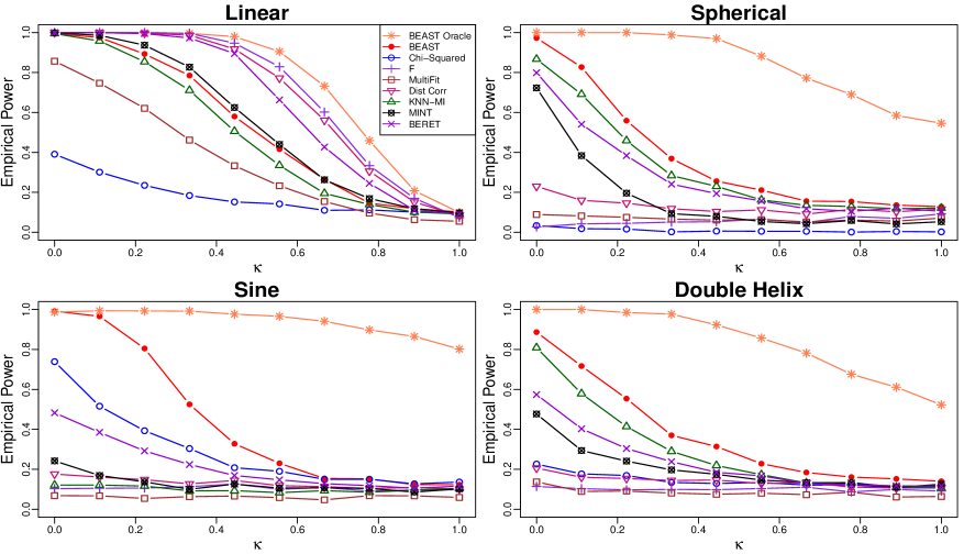
The messages from Figure 2 are similar to those when The BEAST with oracle leads the power under all scenarios to provide a benchmark for feasible power. In particular, under the “Linear” scenario, the gain of the power curve of from those of the -test and the distance correlation demonstrates the ability of to approximate the optimal power. Similar to what we observed in the bivariate cases, the huge margin between the power curve of and other tests indicates the potential substantial gain in power with a proper choice of weights. By approximating the BEAST with oracle, achieves robust power against any form of alternative. The BEAST is particularly powerful against complex nonlinear forms of dependency, and its power curve leads others with a huge margin under all three nonlinear scenarios.
In summary, our simulations in this section show that can approximate the optimal power benchmarked by . The BEAST demonstrates a robust power against many common alternatives in both dimensions or . The BEAST is particularly powerful against a large class of complex nonlinear forms of dependency.
6 Empirical Data Analysis
In this section, we apply the BEAST method to the visually brightest stars from the Hipparcos catalog (Hoffleit and Warren Jr, 1987; Perryman et al., 1997). For each star, a number of features about its location and brightness are recorded. Here, we are interested in detecting if there exists any dependence between the joint galactic coordinates () and the brightness of stars. We consider the absolute magnitude in this section, while study the visual magnitude in the Supplementary Materials. We consider the BEAST, -test, -test, distant correlation (Dist Corr), KNN-MI, MINT, and MultiFIT to this problem. The -values of all the approaches are summarized in Table 3. The BEAST is constructed with , , , and defined in (5.1) where .
| BEAST | Dist Corr | -test | -test | MultiFIT | KNN-MI | MINT | |
| -value | 0 | 0 | 0.091 | 6e-5 | 0.011 | 0.34 | 0.01 |
When testing the independence between the absolute magnitude and the galactic coordinates, this hypothesis is significant based on all the methods except KNN-MI. In addition to producing -values, the BEAST is capable to provide interpretation of the dependence while most competing methods cannot. Hence, we investigated the most important binary interaction among all possible combinations when analyzing the absolute magnitude. From each subsample, we record the most significant binary interaction. The most frequently occurred such interaction is
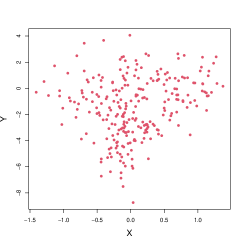
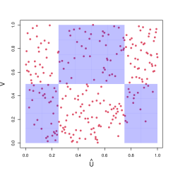
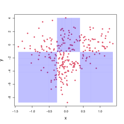
Note that for this with a first row of ’s, the first dimension (the galactic longitude) is not involved. In Figure 3, we plot the absolute magnitude against the galactic latitude. The left panel is the scatter plot of these two variables; the middle panel is the scatter plot after the copula transformation, grouped according to the aforementioned , with the white regions indicating positive interaction and blue regions indicating negative interaction; the right panel is the scatter plot on the original scale when grouped according to the same . The symmetry statistic for is , resulting in a -statistic of for testing the balance of points in white regions and blue regions. Among these stars with the most absolute magnitude, the majority of them are placed between and in latitude. Note that in the galactic coordinate system, the fundamental plane is approximately the galactic plane of the Milky Way galaxy. Therefore, the most frequent binary interaction makes scientific sense for the statistical significance: the bright stars in the data are around the fundamental plane of the Milky Way galaxy. This clear scientific interpretation of the statistical significance is an advantage of the BEAST and the general BET framework.
7 Summary and Discussions
We study the classical problem of nonparametric dependence detection through a novel perspective of binary expansion. The novel insights from the extension of the Euler formula and the binary expansion approximation of uniformity (BEAUTY) shed lights on the unification of important tests into the novel framework of the binary expansion adaptive symmetry test (BEAST), which considers a data-adaptively weighted sum of symmetry statistics from the binary expansion. The one-dimensional oracle on the weights leads to a benchmark of optimal power for nonparametric tests while being agnostic of the alternative. By approximating the oracle weights with resampling and regularization, the proposed BEAST demonstrates consistent performance and is effectively powerful against a variety of complex dependency forms, showcasing its potential across diverse scenarios.
Our study on powerful nonparametric tests of uniformity can be further extended and generalized to many directions. For example, extensions to general goodness-of-fit tests and two-sample tests can be investigated through the BEAST approach. Recent papers in these directions include Brown and Zhang (2023); Zhao et al. (2023a). Tests of other distributional properties related to uniformity, such as tests of Gaussianity and tests of multivariate symmetry can also be studied through the BEAST approach. Insights from these tests can be used in constructing distribution-free models of dependence Brown et al. (2022).
With Theorem 2.2, we further observe that for two arbitrary random vectors and distributed within and respectively, by comparing the characteristic function of the joint distribution and the product of marginal characteristic distributions, the null hypothesis that and are independent is equivalent to the following hypothesis over the expectations of ’s:
With this insight, we propose to study this general test of independence between random vectors in future work. In particular, we plan to study the connection between smooth forms of dependency and the order of binary interactions. A good understanding of this connection can help the development of distribution-free tests targeting at smooth forms of dependence.
Our simulation studies show a gap in empirical power between the BEAST and the BEAST with oracle. Thus the optimal trade-off between sample size, dimension, the depth of binary expansion, and the strength of the non-uniformity would be another interesting problem for investigation. The optimal subsampling and thresholding procedures are critical as well. Results on these problems would lead to a BEAST that is adaptively optimal for a wide class of distributions in power.
Software
The R function BEAST is freely available in the R package of BET.
Acknowledgement
Zhang’s research was partially supported by NSF DMS-1613112, NSF IIS-1633212, NSF DMS-1916237 and DMS-2152289. Zhao’s research was partially supported by NSF IIS-1633283 and DMS-2311216. Zhou’s research was partially supported by NSF-IIS 1545994, NSF IOS-1922701, DOE DE-SC0018344. The authors thank Dr. Xiao-Li Meng and Dr. David Donoho for their generous and insightful comments that substantially improve the paper.
References
- Anderson and Darling [1954] T. W. Anderson and D. A. Darling. A test of goodness of fit. Journal of the American statistical association, 49(268):765–769, 1954.
- Balakrishnan and Wasserman [2019a] S. Balakrishnan and L. Wasserman. Hypothesis testing for densities and high-dimensional multinomials: Sharp local minimax rates. The Annals of Statistics, 47(4):1893 – 1927, 2019a. doi: 10.1214/18-AOS1729. URL https://doi.org/10.1214/18-AOS1729.
- Balakrishnan and Wasserman [2019b] S. Balakrishnan and L. Wasserman. Hypothesis testing for densities and high-dimensional multinomials: Sharp local minimax rates. The Annals of Statistics, 47(4):1893 – 1927, 2019b. doi: 10.1214/18-AOS1729. URL https://doi.org/10.1214/18-AOS1729.
- Barber and Candès [2019] R. F. Barber and E. J. Candès. A knockoff filter for high-dimensional selective inference. The Annals of Statistics, 47(5):2504–2537, 2019.
- Barber and Janson [2022] R. F. Barber and L. Janson. Testing goodness-of-fit and conditional independence with approximate co-sufficient sampling. The Annals of Statistics, 50(5):2514–2544, 2022.
- Barron [1989] A. R. Barron. Uniformly powerful goodness of fit tests. The Annals of Statistics, pages 107–124, 1989.
- Berrett and Samworth [2019] T. B. Berrett and R. J. Samworth. Nonparametric independence testing via mutual information. Biometrika, 106(3):547–566, 2019.
- Berrett and Samworth [2021] T. B. Berrett and R. J. Samworth. Usp: an independence test that improves on pearson’s chi-squared and the g-test. Proceedings of the Royal Society A, 477(2256):20210549, 2021.
- Berrett et al. [2021] T. B. Berrett, I. Kontoyiannis, and R. J. Samworth. Optimal rates for independence testing via u-statistic permutation tests. The Annals of Statistics, 49(5):2457–2490, 2021.
- Blum et al. [1961] J. R. Blum, J. Kiefer, and M. Rosenblatt. Distribution Free Tests of Independence Based on the Sample Distribution Function. The Annals of Mathematical Statistics, 32(2):485 – 498, 1961. doi: 10.1214/aoms/1177705055. URL https://doi.org/10.1214/aoms/1177705055.
- Box et al. [2005] G. E. Box, J. S. Hunter, and W. G. Hunter. Statistics for experimenters: design, innovation, and discovery, volume 2. Wiley-Interscience New York, 2005.
- Brown and Zhang [2023] B. Brown and K. Zhang. The AUGUST two-sample test: Powerful, interpretable, and fast. The New England Journal of Statistics in Data Science, (accepted), 2023.
- Brown et al. [2022] B. Brown, K. Zhang, and X.-L. Meng. Belief in dependence: Leveraging atomic linearity in data bits for rethinking generalized linear models. arXiv preprint arXiv:2210.10852, 2022.
- Cao and Bickel [2020] S. Cao and P. J. Bickel. Correlations with tailored extremal properties. arXiv preprint arXiv:2008.10177, 2020.
- Chatterjee [2020] S. Chatterjee. A new coefficient of correlation. Journal of the American Statistical Association, page in press, 2020.
- Cox [1975] D. Cox. A note on data-splitting for the evaluation of significance levels. Biometrika, 62(2):441–444, 1975.
- Cox and Reid [2000] D. R. Cox and N. Reid. The theory of the design of experiments. CRC Press, 2000.
- Cressie and Read [1984] N. Cressie and T. R. Read. Multinomial goodness-of-fit tests. Journal of the Royal Statistical Society: Series B (Methodological), 46(3):440–464, 1984.
- Dai et al. [2020] C. Dai, B. Lin, X. Xing, and J. Liu. False discovery rate control via data splitting. arXiv preprint arXiv:2002.08542v1, 2020.
- Deb et al. [2020] N. Deb, P. Ghosal, and B. Sen. Measuring association on topological spaces using kernels and geometric graphs. arXiv preprint arXiv:2010.01768, 2020.
- Diaz Rivero and Dvorkin [2020] A. Diaz Rivero and C. Dvorkin. Flow-based likelihoods for non-gaussian inference. Phys. Rev. D, 102:103507, Nov 2020. doi: 10.1103/PhysRevD.102.103507. URL https://link.aps.org/doi/10.1103/PhysRevD.102.103507.
- Donoho and Johnstone [1994] D. L. Donoho and J. M. Johnstone. Ideal spatial adaptation by wavelet shrinkage. Biometrika, 81(3):425–455, 1994.
- Efron and Tibshirani [1994] B. Efron and R. J. Tibshirani. An introduction to the bootstrap. CRC press, 1994.
- Escanciano [2006] J. C. Escanciano. Goodness-of-fit tests for linear and nonlinear time series models. Journal of the American Statistical Association, 101(474):531–541, 2006.
- Fan and Huang [2001] J. Fan and L.-S. Huang. Goodness-of-fit tests for parametric regression models. Journal of the American Statistical Association, 96(454):640–652, 2001.
- Fan et al. [2019] J. Fan, Y. Ke, Q. Sun, and W. Zhou. Farmtest: Factor-adjusted robust multiple testing with approximate false discovery control. Journal of the American Statistical Association, 114(528):1880–1893, 2019.
- Geenens and de Micheaux [2020] G. Geenens and P. de Micheaux. The hellinger correlation. Journal of the American Statistical Association, page in press, 2020.
- Genest and Verret [2005] C. Genest and F. Verret. Locally most powerful rank tests of independence for copula models. Nonparametric Statistics, 17(5):521–539, 2005.
- Genest et al. [2006] C. Genest, J.-F. Quessy, and B. Rémillard. Goodness-of-fit procedures for copula models based on the probability integral transformation. Scandinavian Journal of Statistics, 33(2):337–366, 2006.
- Genest et al. [2009] C. Genest, B. Rémillard, and D. Beaudoin. Goodness-of-fit tests for copulas: A review and a power study. Insurance: Mathematics and economics, 44(2):199–213, 2009.
- Genest et al. [2019] C. Genest, J. Nešlehová, B. Rémillard, and O. Murphy. Testing for independence in arbitrary distributions. Biometrika, 106(1):47–68, 2019.
- Golubov et al. [2012] B. Golubov, A. Efimov, and V. Skvortsov. Walsh series and transforms: theory and applications, volume 64. Springer Science & Business Media, 2012.
- González-Manteiga and Crujeiras [2013] W. González-Manteiga and R. M. Crujeiras. An updated review of goodness-of-fit tests for regression models. Test, 22:361–411, 2013.
- Gorsky and Ma [2018] S. Gorsky and L. Ma. Multiscale Fisher’s independence test for multivariate dependence. arXiv preprint arXiv:1806.06777, 2018.
- Gretton et al. [2007] A. Gretton, K. Fukumizu, C. H. Teo, L. Song, B. Schölkopf, and A. J. Smola. A kernel statistical test of independence. In Advances in neural information processing systems, pages 585–592, 2007.
- Harmuth [2013] H. Harmuth. Transmission of Information by Orthogonal Functions. Springer Berlin Heidelberg, 2013. ISBN 9783662132272. URL https://books.google.com/books?id=O67wCAAAQBAJ.
- Hartigan [1969] J. Hartigan. Using subsample values as typical values. Journal of the American Statistical Association, 64(328):1303–1317, 1969.
- Heller and Heller [2016] R. Heller and Y. Heller. Multivariate tests of association based on univariate tests. In D. D. Lee, M. Sugiyama, U. V. Luxburg, I. Guyon, and R. Garnett, editors, Advances in Neural Information Processing Systems 29, pages 208–216. Curran Associates, Inc., 2016. URL http://papers.nips.cc/paper/6220-multivariate-tests-of-association-based-on-univariate-tests.pdf.
- Heller et al. [2013] R. Heller, Y. Heller, and M. Gorfine. A consistent multivariate test of association based on ranks of distances. Biometrika, 100(2):503–510, 2013.
- Heller et al. [2016] R. Heller, Y. Heller, S. Kaufman, B. Brill, and M. Gorfine. Consistent distribution-free -sample and independence tests for univariate random variables. Journal of Machine Learning Research, 17(29):1–54, 2016.
- Hoeffding [1948] W. Hoeffding. A non-parametric test of independence. The Annals of Mathematical Statistics, pages 546–557, 1948.
- Hoffleit and Warren Jr [1987] D. Hoffleit and W. Warren Jr. The bright star catalogue. ADCBu, 1(4), 1987.
- Huang [2015] Y. Huang. Projection test for high-dimensional mean vectors with optimal direction. PhD thesis, Dept. of Stat., The Pennsylvania State University, 2015.
- Ignatiadis et al. [2016] N. Ignatiadis, B. Klaus, J. Zaugg, and W. Huber. Data-driven hypothesis weighting increases detection power in genome-scale multiple testing. Nature Methods, 13(7):577–580, 2016.
- Jager and Wellner [2007] L. Jager and J. A. Wellner. Goodness-of-fit tests via phi-divergences. Annals of Statistics, 35(5):2018–2053, 2007.
- Janková et al. [2020] J. Janková, R. D. Shah, P. Bühlmann, and R. J. Samworth. Goodness-of-fit testing in high dimensional generalized linear models. Journal of the Royal Statistical Society Series B: Statistical Methodology, 82(3):773–795, 2020.
- Jin and Matteson [2018] Z. Jin and D. Matteson. Generalizing distance covariance to measure and test multivariate mutual dependence via complete and incomplete v-statistics. Journal of Multivariate Analysis, 168:304–322, 2018.
- Kac [1959] M. Kac. Statistical independence in probability, analysis and number theory, volume 134. Mathematical Association of America, 1959.
- Kaiser and Soumendra [2012] M. S. Kaiser and N. Soumendra. Goodness of fit tests for a class of markov random field models. The Annals of Statistics, 40(1):104–130, 2012.
- Kim and Ramdas [2020] I. Kim and A. Ramdas. Dimension-agnostic inference. arXiv preprint arXiv:2011.05068, 2020.
- Kinney and Atwal [2014] J. Kinney and G. Atwal. Equitability, mutual information, and the maximal information coefficient. Proceedings of the National Academy of Sciences, 111(9):3354–3359, 2014.
- Kojadinovic and Holmes [2009] I. Kojadinovic and M. Holmes. Tests of independence among continuous random vectors based on cramér–von mises functionals of the empirical copula process. Journal of Multivariate Analysis, 100(6):1137–1154, 2009.
- LeCam [1973] L. LeCam. Convergence of estimates under dimensionality restrictions. The Annals of Statistics, pages 38–53, 1973.
- Lee et al. [2023] D. Lee, K. Zhang, and M. R. Kosorok. The binary expansion randomized ensemble test. Statistica Sinica, 33(4), 2023.
- Lehmann and Romano [2006] E. L. Lehmann and J. P. Romano. Testing statistical hypotheses. Springer Science & Business Media, 2006.
- Liang et al. [2001] J.-J. Liang, K.-T. Fang, F. Hickernell, and R. Li. Testing multivariate uniformity and its applications. Mathematics of Computation, 70(233):337–355, 2001.
- Liu et al. [2019] W. Liu, X. Yu, and R. Li. Multiple-splitting projection test for high-dimensional mean vectors. Dept. of Stat., Stanford University, 2019. Unpublished.
- Lynn [1973] P. A. Lynn. An introduction to the analysis and processing of signals. McMillan, 1973.
- Ma and Mao [2019] L. Ma and J. Mao. Fisher exact scanning for dependency. Journal of the American Statistical Association, 114(525):245–258, 2019.
- Miller and Siegmund [1982] R. Miller and D. Siegmund. Maximally selected chi square statistics. Biometrics, 38(4):1011–1016, 1982.
- Nelsen [2007] R. B. Nelsen. An introduction to copulas. Springer Science & Business Media, 2007.
- Neyman and Pearson [1933] J. Neyman and E. Pearson. Ix. on the problem of the most efficient tests of statistical hypotheses. Philosophical Transactions of the Royal Society of London. Series A, 231:289–337, 1933.
- Pearl [1971] J. Pearl. Application of walsh transform to statistical analysis. IEEE Transactions on Systems, Man, and Cybernetics, SMC-1(2):111–119, 1971. ISSN 0018-9472. doi: 10.1109/TSMC.1971.4308267.
- Perryman et al. [1997] M. Perryman, L. Lindegren, J. Kovalevsky, E. Hoeg, U. Bastian, P. Bernacca, M. Crézé, F. Donati, M. Grenon, M. Grewing, and F. Van Leeuwen. The hipparcos catalogue. Astronomy and Astrophysics, 323(1):49–52, 1997.
- Pfister et al. [2016] N. Pfister, P. Bühlmann, B. Schölkopf, and J. Peters. Kernel-based tests for joint independence. arXiv preprint arXiv:1603.00285, 2016.
- Politis et al. [1999] D. N. Politis, J. P. Romano, and M. Wolf. Subsampling. Springer, New York, 1999. ISBN 0387988548 9780387988542. URL http://www.worldcat.org/search?qt=worldcat_org_all&q=9780387988542.
- Reshef et al. [2011] D. N. Reshef, Y. A. Reshef, H. K. Finucane, S. R. Grossman, G. McVean, P. J. Turnbaugh, E. S. Lander, M. Mitzenmacher, and P. C. Sabeti. Detecting novel associations in large data sets. Science, 334(6062):1518–1524, 2011.
- Romano and DiCiccio [2019] J. Romano and C. DiCiccio. Multiple data splitting for testing. Department of Statistics, Stanford University, 2019. Unpublished manuscript.
- Sejdinovic et al. [2014] D. Sejdinovic, B. Sriperumbudur, A. Gretton, and K. Fukumizu. Equivalence of distance-based and RKHS-based statistics in hypothesis testing. The Annals of Statistics, 10(5):2263–2291, 2014.
- Sen and Sen [2014] A. Sen and B. Sen. Testing independence and goodness-of-fit in linear models. Biometrika, 101(4):927–942, 2014.
- Shi et al. [2020] H. Shi, M. Hallin, M. Drton, and F. Han. Rate-optimality of consistent distribution-free tests of independence based on center-outward ranks and signs. arXiv preprint arXiv:2007.02186, 2020.
- Spearman [1904] C. Spearman. The proof and measurement of association between two things. The American Journal of Psychology, 15(1):72–101, 1904.
- Stephens [1976] M. A. Stephens. Asymptotic results for goodness-of-fit statistics with unknown parameters. The Annals of Statistics, 4(2):357–369, 1976.
- Székely et al. [2007] G. J. Székely, M. L. Rizzo, and N. K. Bakirov. Measuring and testing dependence by correlation of distances. The Annals of Statistics, 35(6):2769–2794, 12 2007. doi: 10.1214/009053607000000505. URL http://dx.doi.org/10.1214/009053607000000505.
- Wasserman [2006] L. Wasserman. All of Nonparametric Statistics. Springer Texts in Statistics. Springer New York, 2006. ISBN 9780387306230. URL https://books.google.com/books?id=MRFlzQfRg7UC.
- Wasserman and Roeder [2009] L. Wasserman and K. Roeder. High dimensional variable selection. The Annals of Statistics, 37(5A):2178–2201, 2009.
- Xiang et al. [2022] S. Xiang, W. Zhang, S. Liu, C. M. Perou, K. Zhang, and J. Marron. Pairwise nonlinear dependence analysis of genomic data. Annals of Applied Statistics, 2022.
- Zhang [2002] J. Zhang. Powerful goodness-of-fit tests based on the likelihood ratio. Journal of the Royal Statistical Society: Series B (Statistical Methodology), 64(2):281–294, 2002.
- Zhang [2019] K. Zhang. BET on independence. Journal of the American Statistical Association, 114(528):1620–1637, 2019. doi: 10.1080/01621459.2018.1537921. URL https://doi.org/10.1080/01621459.2018.1537921.
- Zhao et al. [2023a] Z. Zhao, K. Zhang, and W. Zhou. Bit by bit: The universal binary coding of random variables in statistics. 2023a. Technical report.
- Zhao et al. [2023b] Z. Zhao, W. Zhang, M. Baiocchi, Y. Li, and K. Zhang. Fast, flexible, and powerful: Introducing a scalable, bitwise framework for non-parametric testing for dependence structure. Techinical report, 2023b.
- Zheng et al. [2012] S. Zheng, N.-Z. Shi, and Z. Zhang. Generalized measures of correlation for asymmetry, nonlinearity, and beyond. Journal of the American Statistical Association, 107(499):1239–1252, 2012.
- Zhu et al. [2017] L. Zhu, K. Xu, R. Li, and W. Zhong. Projection correlation between two random vectors. Biometrika, 104(4):829–843, 2017.