Beamforming for PIN Diode-Based IRS-Assisted Systems Under a Phase Shift-Dependent Power Consumption Model
Abstract
Intelligent reflecting surfaces (IRSs) have been regarded as a promising enabler for future wireless communication systems due to their capability of customizing favorable propagation environments. In the literature, IRSs have been considered power-free or assumed to have constant power consumption. However, recent experimental results have shown that for positive-intrinsic-negative (PIN) diode-based IRSs, the power consumption dynamically changes with the phase shift configuration, which implies that the beamforming quality of the IRS depends on the available power. Therefore, this phase shift-dependent power consumption (PS-DPC) introduces a challenging power allocation problem between the base station (BS) and the IRS, aiming to balance the BS transmit power and the IRS beamforming quality during system design. To tackle this issue, in this paper, we investigate a rate maximization problem for IRS-assisted systems under a practical PS-DPC model. For the single-user case, we propose a generalized Benders decomposition-based beamforming method to maximize the achievable rate while satisfying a total system power consumption constraint. Moreover, we propose a low-complexity beamforming design, where the powers allocated to BS and IRS are optimized offline based on statistical channel state information. Furthermore, we extend the beamforming design to the multi-user case, where we solve an equivalent weighted mean square error minimization problem with two different joint power allocation and phase shift optimization methods. Simulation results indicate that compared to baseline schemes, our proposed methods can flexibly optimize the power allocation between BS and IRS, thus achieving better performance. The optimized power allocation strategy strongly depends on the system power budget. Specifically, when the provided system power budget is high, the PS-DPC is not the dominant factor in the system power consumption, allowing the IRS to turn on as many PIN diodes as needed to achieve high beamforming quality. When the system power budget is limited, however, more power tends to be allocated to the BS to enhance the transmit power, resulting in a lower beamforming quality at the IRS due to the reduced PS-DPC budget.
Index Terms:
Generalized Benders decomposition, intelligent reflecting surface, mixed-integer programming, phase shift-dependent power consumption, power allocation.I Introduction
Intelligent reflecting surfaces (IRSs) have recently attracted increasing attention for the development of next-generation mobile communication systems, as they provide a new communication paradigm to reconfigure the wireless propagation environment [2], [3]. In particular, IRSs are a type of reconfigurable metasurface with a large number of scattering elements. By smartly designing the phase shift of each element, IRSs can flexibly direct the reflected beams into the desired directions, thereby enhancing the coverage and throughput of wireless communication systems [4]. Owing to this promising capability, IRSs have been employed for different purposes in communication systems, e.g., multiple-input multiple-output (MIMO) communications [5], [6], unmanned aerial vehicle communication [7], [8], and physical layer security [9], [10].
Although there are several works evaluating the energy efficiency of IRS-assisted systems [11], [12], the power consumption of the IRS itself is not fully understood, yet. In most of the existing literature, IRSs are assumed to not consume any power or have a constant power consumption that is independent of the phase shift configuration of the IRS. For instance, the authors in [11] investigated the energy efficiency optimization of an IRS-assisted system, where the power consumption of the IRS was modeled as a function of the number of scattering elements and their bit resolution, and assumed to be independent of the phase shift configuration. The resulting constant IRS power consumption model was also employed in [13] to maximize the resource efficiency, which is a performance metric that reflects the trade-off between energy and spectral efficiency. The authors of [12] further studied a system with distributed IRSs, where each IRS can be switched on or off to maximize energy efficiency. It was assumed that the IRSs in the on-state can serve the users by reflecting impinging signals, yet with a constant power consumption. The IRSs in the off-state, on the other hand, did not reflect signals, and were assumed to not consume any power. In addition, the authors of [14] considered the charging and discharging power needed for state switching of the scattering elements, and investigated signal-to-noise ratio (SNR) maximization and energy harvesting in IRS-assisted systems. However, in the above works, the power consumption of the IRSs was assumed to be independent of its phase shift design. Hence, the IRS elements can be arbitrarily reconfigured without affecting the system power consumption.
Contrary to the phase shift-independent power consumption model in the literature, recent experimental results indicate that for the most prevailing types of IRSs, e.g., positive-intrinsic-negative (PIN) diode-based IRSs, the power consumption varies dynamically depending on the states of the PIN diodes [15], [16], [17]111In this paper, we focus on the power consumption model and system optimization of PIN diode-based IRS-assisted systems. It is important to note, however, that several other types of IRSs exist, e.g., varactor-diode-based IRSs, RF switch-based IRSs, etc. [16], [17]. Investigating the power consumption models and the resulting system optimization problem for these other types of IRSs presents an interesting topic for future research.. This phenomenon is primarily due to the disparate power requirements of PIN diodes in the on- and off-states. In particular, a single on-state PIN diode consumes [16], whereas it consumes no power in the off-state. Therefore, the dynamic power consumption of an IRS is proportional to the number of PIN diodes in the on-state. Since the PIN diodes control the phase shift design of the scattering elements, this dynamic power consumption is strongly related to the phase shifts of the IRS elements. Hence, in the remainder of this paper, we refer to this dynamic power consumption as phase shift-dependent power consumption (PS-DPC).
Given the PS-DPC, the beamforming quality of the IRS depends on the available power. To provide high-quality beamforming, the IRS may need to turn on many PIN diodes, thus resulting in a high PS-DPC. However, if the PS-DPC budget is restricted, most PIN diodes have to be turned off, which will seriously affect the degrees of freedom (DoFs) for IRS beamforming. Thus, it is necessary to revisit IRS beamforming design to achieve a good balance between the beamforming quality and the PS-DPC.
Furthermore, due to the large number of scattering elements in IRSs, the PS-DPC of IRSs can be quite high. For example, an IRS prototype with 3600 1-bit scattering elements can consume up to [16], which is no longer negligible compared to the transmit power at the base station (BS) in a downlink system. In such cases, communication operators may care about the total system power consumption, as they need to pay for the power consumption of both the BS and the IRS. Therefore, IRS-assisted downlink communication systems with PS-DPC must contend with a total system power constraint that includes the consumption at both the transmitter and the IRS. This system power constraint necessitates a careful balance of the system power distribution between BS and IRS. Specifically, with a fixed system power budget, allocating more power to the BS can enhance the strength of the transmitted signal, but may reduce the power budget available to the IRS. As mentioned above, such a reduction may diminish the passive beamforming DoF at the IRS, adversely impacting the performance of the overall communication system. Therefore, striking an optimal balance in system power allocation between BS and IRS becomes a critical issue for IRS-assisted systems when considering the PS-DPC. So far, there has been little research on beamforming design for IRS-assisted systems taking into account the PS-DPC. In [18] and [19], the authors adopted the PS-DPC model while seeking to maximize the energy efficiency of an IRS-assisted system. However, while these studies focused on maximizing energy efficiency, the rate maximization problem, which is also a critical issue in wireless communications, remains an unsolved challenge in IRS-assisted systems under the PS-DPC model. Additionally, the authors of [18] and [19] primarily focused on the beamforming optimization under a power constraint at the BS, without exploring beamforming strategies under a more comprehensive power budget constraint for the whole system. As mentioned above, such consideration is crucial, particularly in large IRS-assisted systems, where the PS-DPC is a significant factor in the overall system power budget.
In this paper, we investigate the beamforming design for IRS-assisted systems, where we account for the PS-DPC of PIN diodes, aiming at maximizing the achievable rate in both single-user and multi-user cases. To the best of our knowledge, this is the first attempt to tackle the rate maximization problem of IRS-assisted systems following a PS-DPC model. Our main contributions can be summarized as follows:
-
•
Based on the relationship between the PS-DPC and the IRS coefficients, we formulate a joint power allocation and beamforming optimization problem for IRS-assisted systems under the PS-DPC model. In particular, we maximize the rate of IRS-assisted systems subject to a constraint on the total system power consumption.
-
•
For the single-user case, we develop a generalized Benders decomposition-based beamforming (GBD-BF) method to tackle the rate maximization problem for the PS-DPC model. This method enables joint optimization of active and passive beamforming at BS and IRS, respectively, while limiting the system power consumption.
-
•
Based on statistical channel state information (S-CSI), we further propose a low-complexity beamforming method, where the optimized power allocation strategy between BS and IRS can be optimized offline without frequent updates based on instantaneous CSI.
-
•
In the multi-user case, we transform the sum rate maximization problem into an equivalent weighted mean square error minimization (WMMSE) problem, and propose two novel joint power allocation and beamforming optimization (JPABF) methods to solve it.
-
•
We validate the effectiveness of proposed beamforming methods through computer simulations. The results show that our methods can jointly optimize the power allocation and the beamforming at BS and IRS, thereby enhancing the system performance compared to baseline methods. Specifically, the optimized power allocation strategies depend on the available system power budget. When the power budget is high, the IRS can be allocated a sufficient PS-DPC budget to maximize its beamforming quality. However, for a limited power budget, more power is allocated to the BS to enhance the transmit power, resulting in a lower beamforming quality at the IRS due to the reduced PS-DPC budget.
The remainder of this paper is organized as follows. Section II presents the system model and problem formulation for the considered IRS-assisted system with PS-DPC. Section III derives the GBD-BF method for single-user systems. By further exploiting S-CSI, we develop a low-complexity beamforming method in Section IV. For the multi-user case, Section V proposes two JPABF methods to solve the equivalent WMMSE problem for IRS-assisted systems with PS-DPC. Simulation results are provided in Section VI. Finally, Section VII presents the conclusions of this paper.
Notations: In this paper, represents a column vector, with denoting the -th element of . Similarly, represents a matrix, with denoting the -th element. , , , and denote the transpose, conjugate transpose, conjugate, and trace of a matrix, respectively. denotes the modulus of a scalar. and denote the real and imaginary parts of a scalar, respectively. is the floor function of a real scalar. denotes the remainder of a real scalar after division by 2. and denote the inverse sine and cosine functions of a real scalar in , respectively. is the expectation operator. and denote the Hadamard and Kronecker products, respectively. denotes a diagonal matrix with the elements of on its main diagonal, and is a column vector extracting the diagonal elements of . denotes a block diagonal matrix with diagonal components . denotes the identity matrix. () denotes the all-ones (all-zeros) vector. and denote the sets of real and non-negative real numbers, respectively. denotes the set of all vectors whose elements are restricted to be 1 or 0. represents the set of all complex-valued matrices. denotes the circularly symmetric complex Gaussian distribution with zero mean and covariance matrix . denotes the uniform distribution in .
II System Model and Problem Formulation
II-A Signal Model
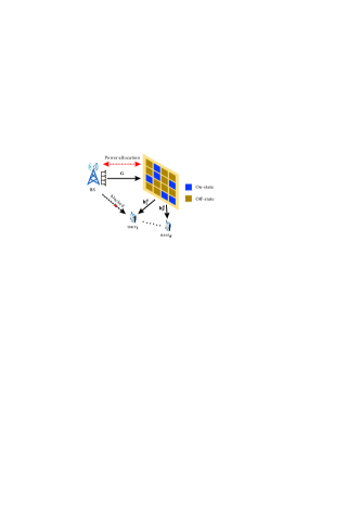
Consider a downlink narrowband multi-user multiple-input single-output (MISO) system as shown in Fig. 1. The system consists of a BS equipped with an -antenna uniform linear array (ULA) and single-antenna users. The direct links between the BS and the users are assumed to be blocked, and thus an IRS is deployed to establish virtual line-of-sight (LoS) links to the users. The IRS is designed as a uniform planar array (UPA) of dimension . The IRS operates with 1-bit phase control resolution, such that the phase shift of each scattering element is binary-switchable between two states through the on/off-state of a PIN diode. Thus, we define as the state vector of the employed PIN diodes, where . For the -th element, () indicates that the corresponding PIN diode is in the on-state (off-state). Without loss of generality, we set the phase shift of the -th element to zero when and when . In this way, the IRS phase shift matrix is given by
| (1) |
Therefore, the equivalent baseband received signal at the -th user can be represented as
| (2) |
where is the BS transmitted symbol vector with , is the active beamforming at the BS, and . represents the additive Gaussian noise at the -th user. denotes the BS-IRS channel matrix, and is the channel vector between the IRS and the -th user.
II-B Channel Model
In this paper, we assume the BS-IRS channel to be Rician distributed comprising one LoS and a number of non-LoSs (NLoSs) links. Hence, denoting the Rician factor by , can be modeled as [20]
| (3) |
where and are the LoS and NLoS components, respectively. Specifically, the LoS component can be characterized by the plane-wave model as , where , , , , and denote the path loss, the angle of departure (AoD), the elevation angle of arrival (AoA), the azimuth AoA of the LoS link, and the carrier wavelength, respectively. The array response vectors for BS and IRS are denoted by and , respectively. By defining , the array response vector of the ULA at the BS can be expressed as . For the UPA at the IRS, the array response vector is given by . The NLoS component , on the other hand, can be expressed as where the elements of matrix are complex Gaussian distributed with mean zero and unit covariance, and the distribution of each element is independent of the other elements.
Similarly, the IRS-user channel is also modeled as Rician fading, i.e.,
| (4) |
where and . , , , and are the Rician factor, the path loss, the LoS elevation AoD, and the LoS azimuth AoD, respectively. In this paper, we assume that and are perfectly known at the BS.
II-C PS-DPC Model of IRSs
The total power consumption of a PIN-diode-based IRS comprises two components [16], [17]. The first one is the static power consumption, which encompasses the energy used by control devices and circuits. The second component is the PS-DPC caused by the PIN diodes, which varies dynamically with respect to the beamforming design at the IRS. Therefore, the total power consumption of the IRS can be modeled as
| (5) |
where and are the static power consumption and the PS-DPC, respectively. As is fixed once the IRS is manufactured, in this paper, we mainly focus on the PS-DPC. Specifically, we consider a 1-bit IRS, where the phase shift of each element is switched between two states according to the on/off-states of a PIN diode. Therefore, the PS-DPC of the IRS can be expressed as follows
| (6) |
where is the power consumption of an on-state PIN diode.
II-D System Power Consumption
In the literature, the transmit power at the BS is typically the only power consumption considered for the wireless system design, regardless of whether [21] or not [22] an IRS is deployed. In contrast, if the PS-DPC of the IRS is also considered, the power consumption of the entire system includes the power consumption of the BS and the IRS, and is given by
| (7) |
where is the BS transmit power consumption. and are the powers consumed by control circuits and each radio frequency chain at the BS, respectively. Note that the power consumption terms in (7) are independent of the beamforming design at BS and IRS, except for and . Thus, we shall focus on the terms for beamforming design in the following.
II-E Problem Formulation
In this paper, we aim to maximize the sum rate of all users under a system power constraint, which leads to the following optimization problem:
| (8) |
where denotes the rate (bps per Hertz) of the -th user, with representing the interference plus noise. Furthermore, is the effective system power budget.
Due to the binary constraint on , problem (8) is a mixed integer nonlinear programming (MINLP) problem, which is nondeterministic polynomial-time (NP)-hard [23]. Moreover, as we account for the PS-DPC, and are coupled in both the objective function and the constraint . This makes the beamforming optimization more challenging than for conventional IRS-assisted rate maximization problems in the literature, where only the power consumption at the BS is considered [6], [21], [24].
Remark 1: In the literature, classical methods such as the alternating optimization (AO) were adopted to tackle the coupling of and [21]. However, this approach cannot be directly applied to solve problem (8) due to the total system power constraint C1. In particular, if the conventional AO algorithm is adopted to solve problem (8), optimizing for a fixed will always lead to an equality in power constraint , i.e., . However, with this condition, the feasible set during the subsequent optimization of is exceedingly small. Specifically, during the optimization in the -th iteration, C1 is reformulated as , where denotes the solution of in the last iteration. This means that during the optimization of , we need to seek a larger achievable rate with fewer on-state PIN diodes, which significantly restricts the IRS’s beamforming DoF. Therefore, applying the conventional AO algorithm for sum rate maximization under the PS-DPC model results in a quick convergence to highly sub-optimal local maxima. To tackle this challenge, in the following sections, we introduce several novel beamforming methods for both the single-user and multi-user cases, which can jointly optimize the power allocation and the beamforming at both the BS and the IRS.
III GBD-BF Method for Single-User Case
In this section, we first start with the single-user case, where the BS serves only one user via the IRS. In this case, denoting and as the IRS-user channel and the active beamforming vector at the BS, respectively, the downlink rate of the user is given by , where is the cascaded channel. Hence, the rate maximization problem in (8) simplifies as follows
| (9) |
To solve this problem, in this section, we propose a novel method to jointly optimize the beamforming at the BS and the IRS based on the GBD algorithm.
III-A Generalized Benders Decomposition
The main idea of the GBD algorithm is to decompose the original MINLP problem into two subproblems, i.e., a primal problem and a master problem, which provide upper and lower bounds for the original problem, respectively [23], [25], [26]. By iteratively solving these two subproblems, the gap between the upper and lower bounds can be progressively reduced, thereby converging towards the optimal solution. To guarantee the convergence of the GBD algorithm, the following two conditions have to be satisfied [23]:
-
•
The problem is convex with respect to the involved continuous variables if the discrete variables are fixed.
-
•
The problem is linear with respect to the involved discrete variables if the continuous variables are fixed.
To be able to employ the GBD algorithm, we first transform the rate maximization problem in (9) into an equivalent problem that maximizes the power of the received signal at the user. This transformation leads to the following problem
| (10) |
Unfortunately, the objective function of (10) is still not suitable for applying the GBD algorithm, as it is non-linear with respect to . However, assuming the optimal solution of (10) is , we notice that is also an optimal solution of (10) for any phase shift . This intrinsic property allows us to choose such that the phase of is rotated to zero. Consequently, we can apply this phase rotation to transform (10) into a more tractable equivalent form:
| (11) |
which satisfies the conditions required for application of the GBD algorithm.
III-B Primal Problem: Beamforming Design at the BS
In the -th iteration, for the primal problem, we fix the discrete variable to the value of the last iteration, i.e., . Thus, problem (11) reduces to an optimization problem with respect to , and is given as
| (12) |
Problem (12) is clearly a convex problem, and the optimal solution, i.e., , can be computed by standard convex program solvers such as CVX [27]. Noticing that is a feasible solution of problem (11), the primal problem can provide an upper bound for problem (11). Furthermore, the Lagrangian function of primal problem (12) can be constructed as
| (13) |
where and are the dual variables for constraints and , respectively.
However, problem (12) may be infeasible for the given , e.g., when . In this case, we consider the following feasibility check problem
| (14) |
where is an auxiliary variable. By denoting and as the dual variables for constraints and , respectively, we can express the Lagrangian for problem (14) as follows
| (15) |
This Lagrangian will be used in the formulation of the master problem, which will be discussed in the next subsection.
III-C Master Problem: Design of the IRS
The master problem of the GBD algorithm is obtained based on the nonlinear convex duality theory [25]. By respectively denoting , and , as the optimal dual solutions of problems (12) and (14) in the -th iteration, the master problem can be formulated as follows
| (16) |
where constraints and represent the optimality and feasibility cuts, respectively. Here, sets and contain the iteration indices for which the primal problem was feasible and infeasible, respectively. The optimal value of the master problem, , establishes a lower bound for problem (10) [25]. However, it is still challenging to directly solve the master problem in (16), because constraints and involve an inner optimization problem related to . To tackle this issue, we further relax the master problem into the variant 2 (V-2) form of GBD [25]. Specifically, constraints and are relaxed by substituting the support functions (the right-hand side parts of constraints and in problem (16)) with their local linear approximations at point . This leads to
| (17) |
According to (13) and (15), and are linear with respect to . Thereby, problem (17) is a mixed integer linear programming (MILP) problem, which can be directly solved by MILP solvers such as MOSEK [27]. The solution obtained, i.e., , is then employed in the primal problem (12) in the next iteration.
III-D GBD-BF Method
The overall GBD-BF scheme is summarized in Algorithm 1. In each iteration, we first fix to the optimal solution in the last iteration, and solve the primal problem or the feasibility check problem to obtain the optimal beamforming vector as well as the optimal dual variables and for the primal problem ( and for the feasibility check problem). Then, the V-2 master problem is solved for fixed , (), and () to obtain for the next iteration. The computational complexity of the GBD-BF method in each iteration is .
IV Low-Complexity S-CSI-BF Method for Single-User Case
In this section, we propose a low-complexity S-CSI-BF method for IRS-assisted single-user systems with PS-DPC. For this method, we first derive the received SNR as a function of the power consumption at the BS and the IRS exploiting S-CSI, and determine the power allocation strategy offline. Then, the beamforming designs at the BS and the IRS are optimized online based on the obtained power allocation.
IV-A The Beamforming Design at the BS and the IRS for Given Power Allocation
We first focus on the online beamforming design at the BS and the IRS for given power allocation, i.e., at the BS and at the IRS. Specifically, as IRSs are generally deployed such that the channels are dominated by the LoS link [3], we ignore the NLoS component for algorithm design for simplicity, thus approximating and as
| (18) |
where and . In this case, the optimal for problem (9) for given is obtained as
| (19) |
where . Therefore, the received SNR at the user can be expressed as:
| (20) |
where and . To maximize the SNR, the continuous phase shift of the -th IRS element without considering the PS-DPC is given by
| (21) |
However, for a 1-bit IRS, the phase shifts of the IRS elements are constrained to binary states, i.e., or . Moreover, due to the PS-DPC, the number of elements with phase shift () is limited by the available power budget for the IRS, i.e., . In this case, by rounding (21) to the binary phase shift states and restricting , the practical phase shift configuration of the -th scattering element is given by
| (22) |
where the set is defined by the following process: First, we sort the elements of in descending order based on their real parts. Then, we select the indices of the top elements from this sorted list to form the set . Here, is defined as , where represents the number of positive elements in .
IV-B The Power Allocation Design
Based on the online beamforming design presented in Section IV-A, in this subsection, we reformulate the received SNR as a function of the power consumption at the BS and the IRS by exploiting S-CSI. Based on this relationship, the power allocation design that satisfies the system power constraint can be optimized offline without frequent updates based on instantaneous CSI.
Specifically, according to the channel model in Section II-B, we can further rewrite as follows
| (23) |
where and . In this case, the elements in have the following property.
Lemma 1
If or is an irrational number, when and , the sequence of all elements in approaches a distribution described by random variable as222Although Lemma 1 is rigorous only when or is an irrational number, our simulations in Section VI shall verify that the proposed S-CSI-BF method is still effective in scenarios where both and are rational numbers.
| (24) |
where .
Proof: Without loss of generality, we assume to be an irrational number. In this case, according to the Weyl’s Equidistribution Theorem [28], the sequence is uniformly distributed in for any when . Furthermore, note that in (23) can be represented by as
| (25) |
As are uniformly distributed in , we can prove that the sequence of all elements of approaches to the distribution described by the random variable in (24), which completes the proof.
Therefore, by assuming and , we can replace by an expectation as follows333Although the number of IRS elements in practical systems is always finite, assuming an infinite number of elements is an efficient asymptotic method to simplify analysis and provide valuable insights. Hence, this approach has been widely applied in previous works [21], [29].
| (26) |
where
| (27) |
with denoting the value corresponding to . Specifically, the probability density function (PDF) of is given by
| (28) |
By further defining , the probability of can be formulated as
| (29) |
which implies that . In this case, we can denote the power consumption at IRS and BS as a function of :
| (30) |
Therefore, the essential part of power allocation optimization is to express the SNR as a function of , and then find the optimal that maximizes the SNR. To achieve this, we further establish two key properties of in the following lemmas.
Lemma 2
Proof: According to (24), we have and . In this case, if , it means with . Therefore, we can further rewrite as
| (31) |
which means as .
Lemma 3
Proof: According to (27) and (28), the PDF of can be written as
| (32) |
therefore, can be calculated by
| (33) |
which completes the proof of Lemma 3.
By exploiting the properties in Lemma 2 and Lemma 3, we ignore the term , and further reformulate the SNR as a function of , which leads to
| (34) |
the maximum of which is given in the following Lemma.
Lemma 4
The maximum of (34) can be found by solving the following equation
| (35) |
Proof: To find the maximum value of the SNR in (34), we first calculate the derivative of the SNR with respect to as
| (36) |
As and tends to zero from below, the derivative in (36) must have at least one zero point, which can be calculated from
| (37) |
For and , the left-hand side of (37) is a decreasing function, while the right-hand side is an increasing function. Therefore, there can only be one zero point of (37), which is the maximum point of (34), i.e., .
IV-C S-CSI-BF Method
The S-CSI-BF method is summarized as follows. In the first step, we obtain the that maximizes the received SNR by solving (35), thus determining the power allocation between BS and IRS offline. With the determined power allocation, the beamforming at the BS and the IRS can then be respectively optimized according to (19) and (22). The complexity of the S-CSI-BF method is , which is mainly attributed to the calculation of and the sorting of .
It should be noted that during the derivation of the S-CSI-BF method, certain approximations were applied, e.g., ignoring the NLoS components of channels (in (18)), assuming and (in (26)), and ignoring the term (in (34)). Despite these simplifications, our numerical results in Section VI shall verify the effectiveness of the S-CSI-BF method. More importantly, the computational complexity of the S-CSI-BF method is much lower than that of the GBD-BF method, as it avoids the high-complexity iteration processes and the MILP master problem in (17).
V JPABF Methods for Multi-User Case
In this section, we further consider the general multi-user case, and reformulate the sum rate maximization problem as an equivalent WMMSE problem. To effectively handle the power allocation challenge introduced by the PS-DPC model, we propose two novel JPABF methods, which enable the joint optimization of the power allocation and the beamforming at the BS and the IRS under the system power constraint.
V-A WMMSE Approach
By referring to [30], we can equivalently transform the sum rate maximization problem (8) into the following WMMSE problem
| (38) |
where , with being an auxiliary variable and . denotes the MSE of the -th user, with , being auxiliary variables. Unfortunately, problem (38) is intractable due to the coupling of multiple optimization variables and the highly non-convex binary constraint on . Hence, a globally optimal solution cannot be obtained in general. To tackle this problem, we apply the AO principle, and alternately optimize the auxiliary variables ( and ) and the beamforming variables (, , and ) to achieve a locally optimal solution of the WMMSE problem. Specifically, by denoting , the solutions of and can be given by
| (39) |
With and determined, problem (38) can then be redefined as the following optimization problem with respect to , , and , excluding constant terms
| (40) |
where , , , and .
Remark 2: In [18] and [19], the authors first considered the energy efficiency maximization problem for an IRS-assisted system with PS-DPC under a BS transmit power constraint. Different from these works, in our study, we focus on the rate maximization problem with a system power constraint including the power consumption at both the BS and the IRS, which is also of great importance in practical applications as noted in Section I. Furthermore, one challenge in the considered problem is that the available power needs to be divided between BS and IRS, which leads to a different design approach compared to those in [18] and [19]. In particular, while the AO algorithm is used in [18] and [19] to alternately update the beamforming at the BS and the IRS, this algorithm is not applicable in this work because it can significantly restrict the IRS’s beamforming DoF, as noted in Remark 1.
V-B JPABF Methods for Beamforming Design
Given the optimized and , in this subsection, we focus on the optimization of , , and . Specifically, to tackle the challenging power allocation problem under the system power constraint, two novel methods are proposed to jointly optimize the power allocation and the beamforming at BS and IRS.
V-B1 JPABF- method
In this method, we first derive closed-form solutions of and for given . Based on the Karush-Kuhn-Tucker (KKT) conditions, the optimal and for (40) are given by
| (41) |
where . To jointly optimize the power allocation and the beamforming design at the BS and the IRS, we further substitute the optimized and , and rewrite the objective function in (40) as a function of . Specifically, note that
| (42) |
Therefore, the objective function in (40) can be rewritten as
| (43) |
where is derived using the Woodbury matrix identity [31]. Note that for the specified in (43), is incorporated not only in matrix but also in coefficient . Now, (40) can be rewritten as the following problem
| (44) |
where is the only optimization variable. Since is obtained by substituting the optimized and , we can ensure that the optimized digital beamforming matrix as well as the corresponding power budget at the BS are updated for each possible . Therefore, by solving (44), we can facilitate the joint optimization of the system power allocation and the beamforming design at BS and IRS.
To solve (44), we apply the coordinate descent (CD) algorithm, and iteratively optimize each element of while keeping the others fixed. Without loss of generality, we assume that the element to be optimized in the current iteration is , which can only be set to 1 or 0. Therefore, we respectively calculate for and , i.e., and , thus determining the optimal as
| (45) |
After the optimization of all elements of , we then determine the optimized and according to (41).
By iteratively optimizing all variables, the overall JPABF- method is summarized in Algorithm 2. As mentioned above, this method facilitates joint power allocation and beamforming design in IRS-assisted systems with PS-DPC. However, it requires the updating of , which necessitates a matrix inversion, in each iteration of the CD algorithm. Consequently, the computational complexity of this method is substantial, on the order of .
V-B2 JPABF- method
To further reduce the computational complexity, in the JPABF- method, we fix and to the solutions obtained in the previous iteration (denoted by and ), and define the BS beamformer as by introducing a power scaling coefficient . Then, we only optimize for each possible in the CD algorithm. In this case, the beamformer at the BS, , can be scaled by the coefficient for each possible , thus also achieving flexible power allocation between BS and IRS. Specifically, we reformulate (38) into the following problem
| (46) |
with objective function
| (47) |
where and . The derivation of (47) eliminates the terms in (40) that are irrelevant to the optimization variables and , and leverages the following matrix properties: , , , and , which hold for any matrices , , and diagonal matrix , where and . Therefore, we can apply a similar CD algorithm to optimize each element in . Specifically, for a given , we note that (46) is a quadratic programming problem for , which has a closed-form solution. Hence, during the optimization of the -th element of , we can respectively calculate for and and the corresponding optimal , i.e., and , thus determining the optimal similar to (45). As objective function is equivalent to that in the original WMMSE problem (38), the and obtained by solving problem (46) can also reduce objective function in (38), thus ensuring the convergence of the JPABF- method. After the optimization of , and are then optimized according to (41).
The JPABF- method is summarized in Algorithm 3. Thanks to the joint optimization of power scaling variable and , the JPABF- method also facilitates flexible power division between BS and IRS during beamforming design. Furthermore, compared to the JPABF- method, the JPABF- method avoids the high-complexity calculations associated with matrix inversion in (43), thus significantly reducing the computational complexity. In particular, the complexity of the JPABF- method is on the order of , which is substantially lower than that of the JPABF- method.
VI Simulation Results
VI-A Simulation Setup
We consider a downlink narrowband IRS-assisted communication system, where the BS is equipped with antennas. The BS is located in the normal direction of the IRS. The distance between BS and IRS is , while the distance from the IRS to the -th user, , follows a uniform distribution in the range of . The other system parameters are presented in Table I.
| Power consumption of an on-state PIN diode | [16] | |
|---|---|---|
| Carrier wavelength | ||
| Noise power at users | ||
| Path loss of the BS-IRS channel | ||
| Path loss of the IRS-UEk channel | ||
| the elevation AoD of | ||
| the azimuth AoD of | ||
| Rician factors of the BS-IRS channel | ||
| Rician factors of the IRS-UEk channel | ||
| the convergence tolerance |
VI-B Baseline Methods
To illustrate the efficiency of the proposed methods, we adopt the following baseline methods for comparison:
-
•
AO, random initialization (AO (rand init)): This method utilizes the conventional AO approach to iteratively optimize the BS beamformer and the IRS configuration. In each iteration, one variable is optimized while the other variables are kept fixed. For the initial state of , , we randomly select the number and locations of the on-state PIN diodes such that the system power constraint is satisfied, i.e., . Therefore, when , the power allocation between BS and IRS is approximately equal in the initial state. If , the initial state is chosen without constraints, leading to approximately half of the PIN diodes being turned on.
-
•
AO, zero initialization (AO (zero init)): This method also applies the AO algorithm for beamforming optimization at BS and IRS. In contrast to the AO (rand init) method, all PIN diodes are initially set to the off-state.
-
•
Ignore PS-DPC: In this method, we optimize the system beamforming with the proposed methods while disregarding the PS-DPC at the IRS. Therefore, this method aims to enhance the IRS beamforming quality as much as possible without considering the PS-DPC. For the multi-user case, we respectively use the JPABF- and JPABF- methods to optimize the beamforming designs at the BS and the IRS while disregarding the PS-DPC, which are referred to as Ignore PS-DPC () and Ignore PS-DPC (), respectively.
-
•
Semidefinite programming (SDP) relaxation [18]: This method aims to enhance the energy efficiency in multi-user IRS-assisted systems with PS-DPC for a power constraint at the BS, and utilizes the AO algorithm to optimize the beamforming at the BS and the IRS alternately. At the BS, beamforming is designed using the zero-forcing technique, while at the IRS, it is optimized via an SDP relaxation algorithm.
VI-C Single-User: System Performance versus Power Budget
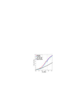
We first evaluate the performance of the proposed methods in the single-user case. In Fig. 2, we plot the downlink rate versus the system power budget for . When , the system power is insufficient to turn on any PIN diodes, leading to a scenario where and only the BS beamforming can be optimized. Consequently, in this low-power regime, all considered beamforming methods converge to a similar rate performance. When , the proposed GBD-BF method consistently achieves the highest rate. This superior performance is attributed to the method’s ability to jointly optimize power allocation and beamforming at the BS and the IRS while taking into account the PS-DPC. On the other hand, the proposed S-CSI-BF method yields competitive performance at high values of , but its effectiveness diminishes at low values of . This is primarily because, when is small, the obtained in (37) is close to . Consequently, is also close to zero. In this scenario, the assumption used in the S-CSI-BF method that is negligible compared to , is no longer fully satisfied, which leads to some performance loss. Nonetheless, the S-CSI-BF method remains highly attractive due to its much lower complexity compared to the GBD-BF method, making it an efficient choice in practical applications.
The conventional AO methods are susceptible to be trapped in local optima close to the initial points, as we have discussed in Remark 1. Specifically, for the AO (zero init) method, remains stuck at . This is beneficial when is low, because turning on PIN diodes would consume a significant portion of the power without substantially improving the IRS’s beamforming capability. However, as increases, the AO (zero init) method experiences a considerable decrease in performance since it cannot leverage the IRS’s beamforming to improve the system rate performance. The AO (rand init) method, conversely, tends to divide the available power evenly between BS and IRS when . As a result, even at low , some PIN diodes remain in the on-state, which can lead to a significant reduction in the transmitted signal power and thus cause a noticeable performance drop.
Finally, as the Ignore PS-DPC method disregards the PS-DPC, it always turns on approximately half of the PIN diodes, leading to a PS-DPC equal to . As a result, this method is not feasible when . For , the Ignore PS-DPC method exhibits lower rates than the proposed methods when the PS-DPC is the dominant factor in the system power budget, specifically for . This is because it disregards the PS-DPC during the optimization of the IRS. However, as continues to increase, the BS becomes the primary consumer of system power. In this high-power regime, the performance of the Ignore PS-DPC method becomes comparable to that of the proposed methods, as the impact of ignoring the PS-DPC diminishes.
To further investigate the power allocation strategies of different methods, we show PS-DPC at the IRS () for different system power budgets in Fig. 3444Since is always 0 for the AO (zero init) method, it is not shown in Fig. 3.. The transmit power of the BS, , can be obtained from . The black dashed line represents the scenario where the power is equally divided between BS and IRS, i.e., . If a method prefers to allocate more power to the IRS, its will exceed the black dashed line, and conversely for less allocated power. As can be observed, conventional AO methods cannot flexibly divide the available power between BS and IRS. In particular, the AO (rand init) method always tends to split the power evenly between BS and IRS when , as its solutions are always trapped at local optima close to the initial states. Similarly, the AO (zero init) method consistently turns off all IRS PIN diodes for all values of , hence allocating all of the system power to the BS. In comparison to the conventional AO methods, the proposed methods demonstrate a more flexible power allocation strategy. Specifically, for lower system power budgets, e.g., , the proposed GBD-BF method favors allocating more power to the BS to enhance the strength of the transmitted signal, reflected in a below the black dashed line. However, when , the system power budget is higher than what is needed to meet the PS-DPC of the IRS. In this case, the PS-DPC is no longer a dominant factor in the system power budget, and the proposed methods can maximize the beamforming quality of the IRS by turning on about half of the PIN diodes. This results in a constant when . Finally, as the Ignore PS-DPC method does not take into account the PS-DPC, it always turns on about half of the PIN diodes, leading to a constant PS-DPC regardless of the system power budget.
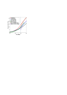
VI-D Single-User: System Performance versus the Size of IRS
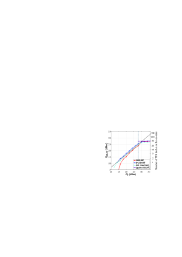
In Fig. 4, we further show the relationship between the achievable rate and the number of IRS elements. As can be observed, the performance of all considered methods monotonically improves as the system power budget and the IRS size increase. Specifically, the proposed GBD-BF method achieves the highest rate for all considered values of and due to its capability of efficiently balancing the power consumption at BS and IRS for beamforming optimization. The proposed S-CSI-BF method approaches the performance of the GBD-BF method when the system power budget is high, but suffers from a performance loss for small values of and large values of . Similar to Fig. 2, this is because the assumption that is negligible compared to , is no longer fully satisfied in these cases. For the AO (rand init) and AO (zero init) methods, as we mentioned above, their solutions are always trapped in local optimal points around the initial states. Therefore, the AO (rand init) method performs better for high , as it can turn on some of the PIN diodes for better beamforming quality. However, when is very low, turning on PIN diodes cannot significantly improve the beamforming quality of the IRS, but will severely reduce the transmit power at the BS. Therefore, the AO (zero init) method outperforms the AO (rand init) method when .
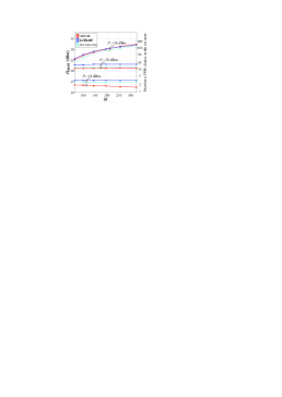
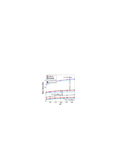
Next, in Fig. 5, we show as a function of . As can be observed, the PS-DPC of all methods depends on the system power budget. When the system power budget is substantial, e.g., , the PS-DPC is not the dominant factor in the system power consumption. In this case, the IRS can improve the beamforming quality by turning on more PIN diodes without significantly affecting the BS transmit power. As a result, the PS-DPC monotonically increases with in this case. Conversely, when the system power is limited, turning on more PIN diodes at the IRS can severely affect the power of the transmitted signals. Therefore, for and , remains almost constant regardless of the IRS size. Specifically, for the proposed GBD-BF method, the PS-DPC may even slightly decrease for larger IRSs when . This can be explained as follows: First of all, when the total power available is very limited, the GBD-BF method tends to allocate more power to the BS as observed in Fig. 3. Given the low power allocated to the IRS, it can only support a small number of PIN diodes in the on-state. In this case, for a large IRS, the impact of altering the states of a few elements is relatively minor due to the extensive number of elements involved. Consequently, turning on only a small number of PIN diodes does not substantially increase the beamforming gain. In contrast, for a smaller IRS, turning on the same number of PIN diodes can lead to a more pronounced improvement in beamforming effectiveness, given the same PS-DPC budget. Therefore, when the total system power consumption is limited, the proposed GBD-BF method allocates more power to an IRS with a smaller size compared to that with a larger size.
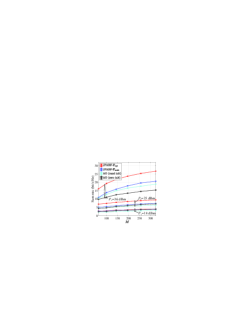
VI-E Multi-User: System Performance versus Power Budget
Now, we evaluate the performance of the proposed methods in the multi-user case. Fig. 6 illustrates the sum rate as a function of when and . As can be observed, the proposed JPABF- method consistently outperforms the baseline methods for all considered , thanks to its capability of jointly optimizing the power allocation and the beamforming at the BS and the IRS. While the JPABF- method exhibits lower performance than the JPABF- method, its complexity is also notably lower, as discussed in Section V.
Regarding the SDP relaxation method from [18], it operates under a BS transmit power constraint rather than a system power constraint. To ensure a fair comparison, we first utilize the SDP relaxation method to design the beamforming under the BS transmit power constraint. Subsequently, we calculate the total system power by summing the powers consumed at both the BS and the IRS. Notably, the SDP relaxation method focuses on maximizing energy efficiency, which peaks around . As a result, even with a larger power consumption budget, it maintains a constant system power consumption around . Therefore, this method fails completely for . Furthermore, it consistently performs worse than the JPABF- method, mainly because the SDP relaxation method uses a less effective zero-forcing algorithm compared to the WMMSE approach employed in this paper. It is also worth noting that the complexity of the SDP relaxation method is very high (), and is notably larger than those of the JPABF- () and JPABF- () methods.
Similar to the single-user case, the conventional AO methods tend to get trapped in suboptimal solutions near their initial values. Therefore, they have significant performance losses compared to the proposed JPABF methods, especially when is high for the AO (zero init) method, and when is low for the AO (rand init) method.
Finally, the Ignore PS-DPC methods show a similar trend as in the single-user case considered in Fig. 2: These methods are not viable when , as about half of the PIN diodes are turned on. They can achieve comparable performance as the proposed methods for large values but suffer a clear performance drop when PS-DPC dominates the system power budget, i.e., for .
VI-F Multi-User: System Performance versus the Size of IRS
In Fig. 7, we show the sum rate versus the number of IRS elements. It can be observed that the proposed JPABF methods outperform the baseline methods for all considered values of . Similar to Fig. 4, the performance gap between the JPABF methods and the AO (zero init) method diminishes for low . In this situation, the JPABF methods also turn off most of the PIN diodes due to the small amount of power available.
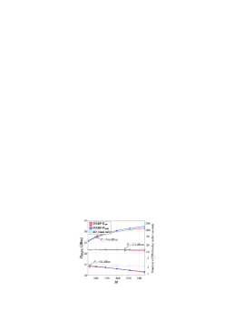
In Fig. 8, we further study the PS-DPC for different IRS sizes. As can be observed, similar power allocation strategies as for the single-user case in Fig. 5 can also be observed for the JPABF methods in the multi-user case. When the system power budget is sufficient, i.e., , the IRS can efficiently design its phase shifts. Therefore, monotonically increases with the IRS size. However, in scenarios where the system power budget is more limited, e.g., when , turning on more PIN diodes can notably reduce the power of the transmitted signals. In this case, an IRS with a larger size even sets more PIN diodes to the off-state, similar to the single-user case in Fig. 5.
VII Conclusion
In this paper, we investigated the rate maximization optimization problem for IRS-assisted systems with PS-DPC. Considering a total system power constraint, the power allocation has been jointly optimized with the beamforming design at the BS and the IRS, leading to a favorable balance between the BS transmit power and the PS-DPC at the IRS. Specifically, for the single-user case, we proposed a GBD-BF method to jointly optimize the power allocation and the beamforming at both BS and IRS. To further reduce the computational complexity, we proposed an S-CSI-BF method, where the optimized power allocation strategy is obtained offline based on S-CSI. For the multi-user case, two JPABF methods were proposed, which could exploit the DoFs introduced by joint BS-IRS power allocation during BS and IRS beamforming optimization based on the WMMSE approach. Simulation results revealed that the proposed methods can flexibly optimize the power allocated to BS and IRS, and thus achieve higher rates than several baseline methods. The obtained power allocation strategies depend on the available system power budget. When the power budget is high, the PS-DPC is not the limiting factor, and the IRS can turn on as many PIN diodes as necessary to achieve optimal beamforming quality. Conversely, for a limited power budget, more power is allocated to the BS to strengthen the transmitted signal, resulting in a reduced PS-DPC budget and, consequently, a lower IRS beamforming quality.
References
- [1] Q. Wu, T. Lin, and Y. Zhu, “Green beamforming design for IRS-aided systems under phase shift-related power consumption,” in Proc. IEEE Global Commun. Conf. (GLOBECOM), Dec. 2023, pp. 613-618.
- [2] M. A. ElMossallamy, H. Zhang, L. Song, K. G. Seddik, Z. Han, and G. Y. Li, “Reconfigurable intelligent surfaces for wireless communications: Principles, challenges, and opportunities,” IEEE Trans. Cogn. Commun. Netw., vol. 6, no. 3, pp. 990-1002, Sept. 2020.
- [3] Q. Wu, S. Zhang, B. Zheng, C. You, and R. Zhang, “Intelligent reflecting surface-aided wireless communications: A tutorial,” IEEE Trans. Commun., vol. 69, no. 5, pp. 3313-3351, May 2021.
- [4] M. Di Renzo et al., “Smart radio environments empowered by reconfigurable intelligent surfaces: How it works, state of research, and the road ahead,” IEEE J. Sel. Areas Commun., vol. 38, no. 11, pp. 2450-2525, Nov. 2020.
- [5] Q. Wu and R. Zhang, “Intelligent reflecting surface enhanced wireless network via joint active and passive beamforming,” IEEE Trans. Wireless Commun., vol. 18, no. 11, pp. 5394-5409, Nov. 2019.
- [6] P. Wang, J. Fang, L. Dai, and H. Li, “Joint transceiver and large intelligent surface design for massive MIMO mmWave systems,” IEEE Trans. Wireless Commun., vol. 20, no. 2, pp. 1052-1064, Feb. 2021.
- [7] X. Pang, M. Sheng, N. Zhao, J. Tang, D. Niyato, and K. -K. Wong, “When UAV meets IRS: Expanding air-ground networks via passive reflection,” IEEE Wireless Commun., vol. 28, no. 5, pp. 164-170, Oct. 2021.
- [8] Z. Wei et al., “Sum-rate maximization for IRS-assisted UAV OFDMA communication systems,” IEEE Trans. Wireless Commun., vol. 20, no. 4, pp. 2530-2550, Apr. 2021.
- [9] X. Yu, D. Xu, Y. Sun, D. W. K. Ng, and R. Schober “Robust and secure wireless communications via intelligent reflecting surfaces,” IEEE J. Sel. Areas Commun., vol. 38, no. 11, pp. 2637-2652, Nov. 2020.
- [10] M. Cui, G. Zhang, and R. Zhang “Secure wireless communication via intelligent reflecting surface,” IEEE Wireless Commun. Lett., vol. 8, no. 5, pp. 1410-1414, Oct. 2019.
- [11] C. Huang, A. Zappone, G. C. Alexandropoulos, M. Debbah, and C. Yuen, “Reconfigurable intelligent surfaces for energy efficiency in wireless communication,” IEEE Trans. Wireless Commun., vol. 18, no. 8, pp. 4157-4170, Aug. 2019.
- [12] Z. Yang et al, “Energy-efficient wireless communications with distributed reconfigurable intelligent surfaces,” IEEE Trans. Wireless Commun., vol. 21, no. 1, pp. 665-679, Jan. 2022.
- [13] L. You, J. Xiong, D. W. K. Ng, C. Yuen, W. Wang, and X. Gao, “Energy efficiency and spectral efficiency tradeoff in RIS-aided multiuser MIMO uplink transmission,” IEEE Trans. Signal Process., vol. 69, pp. 1407–1421, Dec. 2021.
- [14] K. Ntontin et al., “Wireless energy harvesting for autonomous reconfigurable intelligent surface,” IEEE Trans. Green Commun. Netw., vol. 7, no. 1, pp. 114–129, Mar. 2023.
- [15] J.-B. Gros, V. Popov, M. A. Odit, V. Lenets, and G. Lerosey, “A reconfigurable intelligent surface at mmwave based on a binary phase tunable metasurface,” IEEE Open J. Commun. Society, vol. 2, pp. 1055–1064, May 2021.
- [16] J. Wang et al., “Reconfigurable intelligent surface: Power consumption modeling and practical measurement validation,” IEEE Trans. Commun., early access, Mar. 28, 2024, doi: 10.1109/TCOMM.2024.3382332.
- [17] J. Wang, W. Tang, S. Jin, X. Li, and M. Matthaiou, “Static power consumption modeling and measurement of reconfigurable intelligent surfaces,” in Proc. IEEE 31th Eur. Signal Process. Conf. (EUSIPCO), Sept. 2023, pp. 890-894.
- [18] Z. Li, J. Zhang, J. Zhu, S. Jin, and L. Dai, “Enhancing energy efficiency for reconfigurable intelligent surfaces with practical power models,” 2023, arXiv:2310.15901. [Online]. Available: https://arxiv.org/abs/2310.15901.
- [19] D. Xu, Y. Han, X. Li, J. Wang, and S. Jin, “Energy efficiency optimization for a RIS-assisted multi-cell communication system based on a practical RIS power consumption model,” Front. Inf. Technol. Electron. Eng., vol. 24, no. 12, pp. 1717-1727, Jan. 2024.
- [20] S. Zhang et al., “Intelligent omni-surfaces: Ubiquitous wireless transmission by reflective-refractive metasurfaces,” IEEE Trans. Wireless Commun., vol. 21, no. 1, pp. 219-233, Jan. 2022.
- [21] Q. Wu and R. Zhang, “Beamforming optimization for wireless network aided by intelligent reflecting surface with discrete phase shifts,” IEEE Trans. Wireless Commun., vol. 68, no. 3, pp. 1838-1851, Mar. 2020.
- [22] X. Yu, J. -C. Shen, J. Zhang, and K. B. Letaief, “Alternating minimization algorithms for hybrid precoding in millimeter wave MIMO systems,” IEEE J. Sel. Topics Signal Process., vol. 10, no. 3, pp. 485-500, Apr. 2016.
- [23] Y. Wu, D. Xu, D. W. K. Ng, R. Schober, and W. Gerstacker, “Globally optimal resource allocation design for IRS-assisted multiuser networks with discrete phase shifts,” in Proc. IEEE Int. Conf. Commun. Workshops (ICC Workshops), May 2023, pp. 1216-1221.
- [24] H. Guo, Y. -C. Liang, J. Chen and E. G, “Weighted sum-rate maximization for reconfigurable intelligent surface aided wireless networks,” IEEE Trans. Wireless Commun., vol. 19, no. 5, pp. 3064-3076, May 2020.
- [25] A. M. Geoffrion, “Generalized Benders decomposition,” J. Optim. Theory Appl., vol. 10, no. 4, pp. 237–260, Oct. 1972.
- [26] H. Huang, Y. Zhang, H. Zhang, Z. Zhao, C. Zhang, and Z. Han, “Multi-IRS-aided millimeter-wave multi-user MISO systems for power minimization using generalized Benders decomposition,” IEEE Trans. Wireless Commun., vol. 22, no. 11, pp. 7873-7886, Nov. 2023.
- [27] M. Grant and S. Boyd, “CVX: Matlab software for disciplined convex programming, version 2.1,” http://cvxr.com/cvx, Jan. 2020.
- [28] L. Kuipers and H. Niederreiter, Uniform Distribution of Sequences. New York: Wiley-Interscience, 1974.
- [29] J. Xu, Y. Liu, X. Mu, R. Schober, and H. V. Poor, “STAR-RISs: A correlated T&R phase-shift model and practical phase-shift configuration strategies,” IEEE J. Sel. Topics Signal Process., vol. 16, no. 5, pp. 1097-1111, Aug. 2022.
- [30] X. Zhao, T. Lin, Y. Zhu, and J. Zhang, “Partially-connected hybrid beamforming for spectral efficiency maximization via a weighted MMSE equivalence,” IEEE Trans. Wireless Commun., vol. 20, no. 12, pp. 8218-8232, Dec. 2021.
- [31] H. Henderson and S. Searle, “On deriving the inverse of a sum of matrices,” Siam Rev., vol. 23, no. 1, pp. 53–60, Jan. 1981.