BayesNAM: Leveraging Inconsistency for Reliable Explanations
Abstract
Neural additive model (NAM) is a recently proposed explainable artificial intelligence (XAI) method that utilizes neural network-based architectures. Given the advantages of neural networks, NAMs provide intuitive explanations for their predictions with high model performance. In this paper, we analyze a critical yet overlooked phenomenon: NAMs often produce inconsistent explanations, even when using the same architecture and dataset. Traditionally, such inconsistencies have been viewed as issues to be resolved. However, we argue instead that these inconsistencies can provide valuable explanations within the given data model. Through a simple theoretical framework, we demonstrate that these inconsistencies are not mere artifacts but emerge naturally in datasets with multiple important features. To effectively leverage this information, we introduce a novel framework, Bayesian Neural Additive Model (BayesNAM), which integrates Bayesian neural networks and feature dropout, with theoretical proof demonstrating that feature dropout effectively captures model inconsistencies. Our experiments demonstrate that BayesNAM effectively reveals potential problems such as insufficient data or structural limitations of the model, providing more reliable explanations and potential remedies.
1 Introduction
Explainable artificial intelligence (XAI) has become a significant field of research as machine learning models are increasingly applied in real-world systems including finance and healthcare. To provide insight into the underlying decision-making process behind the predictions made by these models, numerous researchers have developed various techniques to assist human decision-makers.
Recently, Agarwal et al.[1] proposed a neural additive model (NAM) that utilizes neural networks to achieve both high performance and explainability. NAM is a type of generalized additive model (GAM) that involves the linear or non-linear transformation of each input and yields the final prediction through an additive operation. Previous studies have demonstrated that NAM not only learns complex relationships between inputs and outputs but also provides a high level of explainability based on neural network architectures and training techniques.

In this paper, we analyze a critical yet overlooked phenomenon: the inconsistency phenomenon of NAM. Fig. 1 illustrates this issue, where two independent NAMs, trained on the same dataset and architecture, produce different explanations due solely to variations in random seeds. Such inconsistency has traditionally been viewed as a problem to be solved [2].
However, we argue that these inconsistencies are not merely obstacles but can offer valuable insights to uncover external explanations within the data model. Through a simple theoretical model, we show that NAMs naturally exhibit the inconsistency phenomenon even when trained on usual datasets that contain multiple important features. Building on this insight, we propose the Bayesian Neural Additive Model (BayesNAM), a novel framework that combines Bayesian neural networks with feature dropout to harness these inconsistencies for more reliable explainability. We also provide theoretical proof that feature dropout effectively leverages inconsistency. Our real-world experiments demonstrate that BayesNAM not only provides more reliable and interpretable explanations but also highlights potential issues in the data model, such as insufficient data and structural limitations within the model.
The main contributions can be summarized as follows:
-
•
We investigate the inconsistency phenomenon of NAMs and analyze this phenomenon through a simple theoretical model.
-
•
We propose a new framework BasyesNAM, which utilizes Bayesian neural network and feature dropout. We also establish a theoretical analysis of the efficacy of feature dropout in leveraging inconsistency information.
-
•
We empirically demonstrate that BayesNAM is particularly effective in identifying data insufficiencies or structural limitations, offering more reliable explanations and insights for decision-making.
2 Related Work
2.1 Neural Additive Model
As numerous machine learning and deep learning models are black-box, a line of work has attempted to explain the decisions made by a black-box model. We call these methods post-hoc methods since they are applied after the model has been trained. While post-hoc methods offer some interpretability, recent work [3, 4] has argued that these methods can lead to unreliable explanations, which could potentially have detrimental effects on their explainability.
In contrast to post-hoc methods, intrinsic methods aim to develop an inherently explainable model without additional techniques [4]. Agarwal et al.[1] proposed a neural additive model (NAM), which combines a generalized additive model [5] and neural networks. To be specific, given features, and a target , NAM constructs mapping functions as follows:
| (1) |
where is a bias term and each mapping function . In Fig. 2, We illustrate an example of NAM. By utilizing the neural network, NAMs capture the non-linear relationship and achieve high performance while maintaining clarity through a straightforward plot.
Despite their strengths, NAMs frequently exhibit inconsistent explanations even when trained on identical datasets with the same architectures, as illustrated in Fig. 1. These inconsistencies can also be observed in the original work [1], where the mapping functions produced by different NAMs within an ensemble show substantial variation, despite being trained under the same experimental conditions.
While this inconsistent phenomenon across NAMs can harm its explainability as they are intended to be XAI models, this phenomenon has received limited attention in the literature. To the best of our knowledge, only one study has explicitly addressed this issue. Radenovic et al. [2] introduced the neural basis model (NBM), which used shared basis functions across features rather than assigning independent mapping functions to each feature. They argued that NBM reduces divergence between models, offering more consistent shape functions compared to NAM, thus mitigating the inconsistency problem.
In contrast, this paper presents a novel view on the inconsistency phenomenon. Rather than treating it as a problem to be solved, we argue that these inconsistencies provide valuable information about the data model.

2.2 Bayesian Neural Network
Although the use of a single model is a fundamental approach, numerous studies have found that a point-estimation is often vulnerable to overfitting and high variance due to its limited representation [6]. To overcome this limitation, Bayesian neural network estimates the model distribution instead of calculating a fixed model. Given the data and the prior , we aim to approximate the posterior . Specifically, rather than using a fixed weight vector , it aims to find a distribution of weight vectors and learn the mean vector and the standard deviation vector .
Since the distribution is generally intractable, several methods have been developed to approximate the posterior, including Markov Chain Monte Carlo (MCMC) [7] and variational inference approaches [8, 9]. While MCMC methods can provide more accurate estimates, their high computational cost [10] has led to the use of variational inference methods across diverse domains [11, 12].
During optimization in variational inference methods, an weight vector is sampled for each forward step where . The prior distribution can be simply chosen as the isometric Gaussian prior where is a predefined standard deviation to explicitly calculate the KL-divergence [11].
A promising direction in the field of Bayesian neural networks is their integration with other domains to enhance model explainability. Bayesian neural networks provide weight distributions that enable the identification of high-density regions or confidence intervals, which can be used for uncertainty estimation. Researchers and practitioners in several domains that require reliable explanations, such as medicine [13] and finance [14], have also explored the utilization of Bayesian models to measure the confidence of prediction for trustworthy decision-making.
3 Methodology
In Section 3.1, we first investigate the inconsistency phenomenon of NAMs with a simple theoretical model. Our empirical findings show that this inconsistency can easily occur, even when datasets contain more than one important feature. Subsequently, in Section 3.2, we propose a new framework called BayesNAM, which combines Bayesian neural network with feature dropout, to leverage the inconsistency information as a source of valuable indicator. This framework is supported by a theoretical analysis demonstrating the effectiveness of feature dropout in capturing diverse explanations. Finally, we provide a detailed explanation of the proposed framework.
3.1 Rethinking Inconsistency of Neural Additive Model


We begin the analysis by identifying and investigating the inconsistent explanations of NAM. To this end, we construct a simple theoretical model. Here, we consider a binary classification task where the target can have a value in . Inspired by [15], we construct the input-target pairs from a distribution as follows:
| (2) | ||||
| (3) |
where are independently and identically sampled from a normal distribution with the mean and the standard deviation for positive and . It is important to note that the features are uncorrelated, as they are drawn independently and identically distributed. By adjusting the values of and , we can control the significance of and in predicting , as stated in the following lemma:
Lemma 1.
(Derived from [15]) Consider a linear classifier ,
| (4) |
Then, even a natural linear classifier, with , can easily achieve a higher classification accuracy than , which is a natural accuracy of the model that only uses , if the following statement is satisfied:
| (5) |
where is the cumulative distribution function of . (Detailed proof is presented in Appendix)
Let be a sufficiently large positive number. When , only is useful to predict and other features are not correlated to . As increases, become correlated to . By Lemma 1, if (5) is satisfied, a model that only considers can achieve a higher classification accuracy than . In summary, if , would be the only feature with a high importance in predicting , while is enough to have a significant performance in predicting for a large .
Now, we consider the following two cases with d=3:
-
•
Case-I. Single important feature exists . In this case, only is effective in predicting , while and are not useful.
-
•
Case-II. Multiple important features exist . In this case, all the features, , , and are highly correlated with . The model uses and can perform better than the model sorely depends on since .
Given this theoretical model, we generated two sets of data containing 50,000 training examples and 10,000 test examples and trained two different NAMs on each dataset for different random seeds. For simplicity, we fixed the feature dimension to , the probability , and , resulting (5) becomes , where is drawn from the standard normal distribution . For each mapping function of NAM, we constructed a simple neural network with two linear layers containing 10 hidden neurons and used ReLU as an activation function. The models are trained by SGD with a learning rate of 0.01. One epoch was sufficient to achieve high training accuracy.


Fig. 3 (Case-I) and Fig. 4 (Case-II) illustrate the mapping functions of trained NAMs for each case. Specifically, for Case-I, we observed that the two NAM models trained with different random seeds exhibited similar test accuracy and explanations (94.9% and 95.0%, respectively). As shown in Fig. 3, the mapping functions for each have similar shapes, with being the only increasing one and the others being almost constant. Therefore, in this case, NAM successfully captures the true importance of features and provides reliable explanations.

In contrast, for Case-II (Fig. 4), the mapping functions of the trained NAMs have extremely different shapes. Although both NAMs achieve a test accuracy exceeding 99.99%, is much steeper than for the first random seed, whereas the relationship is reversed for the second random seed, and vice versa.
Such inconsistency results in inconsistent feature contribution. Figure 5 shows the feature contribution of a sample . Following [1], we calculate the feature contribution by subtracting the average value of a mapping function across the entire training dataset. Although we use the same example, the feature contribution calculated by NAM with random seed 1 implies that appears to be more important than , while NAM with random seed 2 outputs the opposite result that appears to be more significant than . In summary, NAMs can produce inconsistent explanations when multiple important features are present, a common condition in real-world datasets. Indeed, as discussed later in Figures 10 and 12, this inconsistency is readily observable in widely-used datasets.
At first glance, the observed inconsistency may appear problematic; however, both explanations are not inherently incorrect. Specifically, given the theoretical model, both and are important features under Case-II, as using only one of them can achieve high performance. Therefore, the distinct mapping functions demonstrate that the different perspectives of trained models and each explanation is a valid interpretation of the data model, where relying solely on either or is sufficient for high performance.


In Fig. 6, we vary the learning rates () and batch sizes () during training within the same theoretical model. We linearly increase the learning rate from 0.005 to 0.01, and the batch size from 5 to 50. In total, we trained 50 models for each experiment, where each NAM exhibits inconsistent mapping functions. However, it is important to note that all models achieved over 99% test accuracy on the dataset. This indicates that the diverse explanations are not incorrect; rather, they offer valuable external insights into the existence of diverse perspectives among high-performing models, complementing the internal explanations of individual models. Therefore, we posit that inconsistency can be a useful indicator of potential external explanatory factors. Based on these findings, we propose a new framework to leverage inconsistency and provide additional explanations within the data model.
3.2 Bayesian Neural Additive Model
In the previous subsection, we explored the inconsistency phenomenon in NAMs and suggested that rather than being a flaw, this inconsistency can serve as a valuable source of additional information, shedding light on underlying external explanations in the data model. In this section, we introduce BayesNAM, a novel framework designed to leverage this inconsistency. BayesNAM incorporates two key approaches: (1) a modeling approach based on Bayesian structure and (2) an optimization approach utilizing feature dropout. Each of these approaches will be detailed in the following paragraphs.
1) Modeling Approach: Bayesian Structure for Inconsistency Exploration. A naive approach to exploring possible inconsistencies in NAMs is by training multiple independent models. Indeed, Agarwal et al.[1] trained several NAMs and visualized the learned shape functions . However, this requires training independent models, leading to a computational burden proportional to , making it impractical for large-scale applications.
To address this limitation, we propose using Bayesian neural networks [8, 9], which inherently allow for efficient exploration of model uncertainty without the need to train multiple independent models. Under variational inference and Bayes by Backprop [8, 9], Bayesian neural networks rather train the mean parameter and the standard deviation parameter instead of an weight vector . Then, during the training and inference phase, it samples a weight for a random vector from a predefined distribution. Following prior works [11, 12], we adopt the reparameterization trick [16] for efficient training. This results in the following training objective.
| (6) |
where is a given loss function and is the KL-divergence. For further details, we refer the readers to [9].
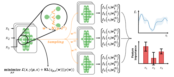
In Fig. 7, we present the structural framework that integrates a Bayesian neural network with a neural additive model. For each sampled weight , we compute the corresponding predictions . This sampling approach enables the model to efficiently explore a diverse range of model spaces without needing to train multiple models. By incorporating a Bayesian neural network, the model provides high-density regions of the mapping functions and provides confidence intervals for feature contributions, offering richer interpretability.


2) Optimization Approach: Feature Dropout for Encouraging Diverse Explanations. Although Bayesian neural networks provide an efficient mechanism for exploration, they do not inherently guarantee exploring diverse explanations. Indeed, as shown in Fig. 8a, naive Bayesian neural network alone tends to focus on a single feature, similar to training a single NAM, rather than adequately exploring diverse explanations. As previously noted in related works [11, 12], we observe that increasing the standard deviation hyper-parameter within Bayesian neural network tends to degrade model performance and fails to address this issue effectively. Therefore, given the presence of diverse valid explanations shown in Figures 4 and 5, it is evident that a method is needed to encourage the exploration of diverse explanations.
As a potential solution, we propose the use of feature dropout during optimization. Feature dropout, initially introduced by Agarwal et al.[1], extends traditional dropout by selectively omitting individual feature networks during training. The hyperparameter determines the probability of dropping each feature. While the original work focused on improving model performance with feature dropout, we here provide a theoretical analysis showing that feature dropout implicitly encourages diverse explanations, preventing over-relying on any single feature.
Given the theoretical model in Section 3.1, we establish the following theorem.
Theorem 1.
(Feature Dropout Implicitly Encourages Exploring Diverse Explanations) Given the dataset in (2), the linear classifier in (4), and the feature dropout rate , without loss of generality, the maximal training accuracy of that only uses features becomes
| (7) |
Then, for and , the gap is always positive and increases as increases. Thus, the model leverages multiple features to achieve high performance, implicitly encouraging the exploration of diverse explanations.
Sketch of proof.
Let . Then, can be formalized as follows:
To show that and for and 8, we use mathematical induction.
Applying Pascal’s identity and strong induction, we find
We now consider two cases for : (1) and (2) . In each case, we prove that by finding the value of that minimizes each term. With these lower bounds, we can conclude that the overall expression is positive. (Detailed proof is presented in Appendix) ∎


Fig. 9 empirically verifies the general acceptance of Theorem 1. We plot with varying . Other settings are same as the Case-II in Section 3.1. The increasing trend of for aligns with the implications of Theorem 1. Furthermore, the acceptable range of in Theorem 1 expands as increases. When , is increasing for . Even for , we observe that increases until . Since Theorem 1 holds regardless of the values of , we observe similar results for a very small value of .
In summary, we theoretically and empirically verify that feature dropout encourages the model to explore diverse explanations by using multiple features in the dataset. As shown in Fig. 8b, incorporating feature dropout enables the model to explore explanations across a range of features. Therefore, we introduce the framework that combines Bayesian neural networks with feature dropout as Bayesian Neural Additive Model (BayesNAM).
4 Experiments
In this section, we present empirical findings comparing the performance of our proposed framework against traditional models, such as Logistic/Linear Regression, Classification and Regression Trees (CART), and Gradient Boosted Trees (XGBoost) [17], as well as recent explainable models including the Explainable Boosting Machine (EBM) [18], NAM, NAM with an ensemble method (NAM+Ens), and our proposed BayesNAM. For Logistic/Linear Regression, CART, XGBoost, and EBM, we conducted a grid search for hyperparameter tuning, following the settings outlined in [1]. We found that using ResNet blocks—comprising two group convolution layers with BatchNorm and ReLU activation—yields better performance for NAM and BayesNAM compared to the ExU units or ReLU- suggested in [1]. For NAM+Ens, we trained five independent NAMs, and both NAM+Ens and BayesNAM utilized soft voting for model aggregation during evaluation. Detailed settings are provided in the Appendix.
We evaluated all models on five different datasets: Credit Fraud [19], FICO [20], and COMPAS [21] for classification tasks, and California Housing (CA Housing) [22] and Boston [23] for regression tasks. As shown in Table I, BayesNAM demonstrates comparable performance to other benchmarks across datasets, with particularly strong results in classification tasks such as COMPAS, Credit Fraud, and FICO. For regression tasks, BayesNAM tends to be less accurate, which we discuss further in the Appendix.
| Model |
|
|
|
|
|
||||||||||
|---|---|---|---|---|---|---|---|---|---|---|---|---|---|---|---|
| Log./Lin. Reg. | 0.6990.005 | 0.9770.004 | 0.7060.005 | 5.5170.009 | 0.7310.010 | ||||||||||
| CART | 0.7760.005 | 0.9560.005 | 0.7840.002 | 4.1330.004 | 0.7120.007 | ||||||||||
| XGBoost | 0.7430.012 | 0.9800.005 | 0.7950.001 | 3.1550.009 | 0.5310.011 | ||||||||||
| EBM | 0.7640.009 | 0.9780.007 | 0.7930.005 | 3.3010.005 | 0.5580.012 | ||||||||||
| NAM | 0.7690.011 | 0.9890.007 | 0.8040.003 | 3.5670.012 | 0.5560.009 | ||||||||||
| NAM+Ens | 0.7710.005 | 0.9900.004 | 0.8040.002 | 3.5550.006 | 0.5540.003 | ||||||||||
| BayesNAM | 0.7840.009 | 0.9910.003 | 0.8040.001 | 3.6200.011 | 0.5560.007 |
4.1 Identifying Data Inefficiency
The capability of BayesNAM to explore diverse explanations further allows us to obtain confidence information of feature contributions. In the left plot of Figure 10, we plot the feature contributions of two randomly drawn offenders from each target value, ‘reoffended’ () or ‘not’ ().


Among the features, juv_other_count (which represents the number of non-felony juvenile offenses a person has been convicted of) exhibits high variance in its contributions. This high variance indicates that, with a single NAM, the contribution of juv_other_count can appear either extremely negative or positive, potentially leading to misinterpretation. BayesNAM reveals substantial variability among models, suggesting that juv_other_count can have both positive and negative effects on predictions within certain ranges.
What can we infer from this high variation? In the right plot of Figure 10, we analyze the mapping function of juv_other_count. NAMs (gray) show inconsistent explanations for juv_other_count. The two-sigma interval of mapping functions of BayesNAM (orange) also starts to diverge significantly when juv_other_count , indicating increased inconsistency in this range. As shown in Figure 11a, a data range where juv_other_count indicates a lack of sufficient data. Moreover, this range also shows skewed proportions, especially for juv_other_count , where all labels are either ’reoffended’ or ’not.’ In summary, we verify that the high inconsistency highlights the need for caution when interpreting examples involving the feature, and suggests potential issues such as a lack of data.
In addition to identifying data insufficiencies, our model can also be used for feature selection. Features with high absolute contributions and small standard deviations, such as priors_count (which represents the total number of prior offenses a person has been convicted of), consistently demonstrate significant impact across different models.
4.2 Capturing Structural Limitation


In addition to data insufficiencies, a high level of inconsistency can reveal structural limitations within the model. In Fig. 12a, we plot the results of NAMs and BayesNAM for longitude. These functions show higher housing prices in San Francisco (around -122.5) and Los Angeles (around -118.5), consistent with previous findings [1]. However, BayesNAM finds that there exist inconsistent explanations between these two cities, particularly within the longitude range of -120 to -119.
We hypothesize that this inconsistency is due to significant variations in housing prices (target variable) across different latitudes. Fig. 12b illustrates the distribution of housing prices in California, with red circles indicating higher prices and larger circles representing higher volumes of houses. As shown in Fig. 12b, while Santa Barbara, Yosemite National Park, and Fresno are on similar longitudes, Santa Barbara exhibits a substantial price gap compared to the others. Additionally, since Yosemite National Park and Fresno are near the same latitude as San Francisco, NAM might struggle to accurately predict housing prices without the interaction term between Latitude and Longitude.
Based on this observation, we train a NAM with an interaction term between Latitude and Longitude. This model achieved a much better performance (RMSE: ) than without the interaction term (RMSE: ). In addition, The significance of the interaction term is particularly evident near Yosemite. When BayesNAM is trained with this interaction term, it also shows reduced variance in the longitude range of -120 to -119. This suggests that the high variance can highlight potential structural limitations within models. Moreover, considering that existing methods such as NA2M [1], which incorporate all possible interaction terms, incur heavy computational costs and diminished explainability, BayesNAM offers a promising alternative by effectively selecting the most important interaction terms.
5 Conclusion
In this work, we identified and analyzed the inconsistent explanations of NAMs. We highlighted the importance of acknowledging these inconsistencies and introduced a new framework, BayesNAM, which leverages inconsistency to provide more reliable explanations. Through empirical validation, we demonstrated that BayesNAM effectively explores diverse explanations and provides external explanations such as insufficient data or model limitations within the data model. We hope our research contributes to the development of trustworthy models.
References
- [1] R. Agarwal, L. Melnick, N. Frosst, X. Zhang, B. Lengerich, R. Caruana, and G. E. Hinton, “Neural additive models: Interpretable machine learning with neural nets,” Advances in Neural Information Processing Systems, vol. 34, pp. 4699–4711, 2021.
- [2] F. Radenovic, A. Dubey, and D. Mahajan, “Neural basis models for interpretability,” Advances in Neural Information Processing Systems, vol. 35, pp. 8414–8426, 2022.
- [3] I. E. Kumar, S. Venkatasubramanian, C. Scheidegger, and S. Friedler, “Problems with shapley-value-based explanations as feature importance measures,” in International Conference on Machine Learning. PMLR, 2020, pp. 5491–5500.
- [4] C. Rudin, “Stop explaining black box machine learning models for high stakes decisions and use interpretable models instead,” Nature Machine Intelligence, vol. 1, no. 5, pp. 206–215, 2019.
- [5] R. Hastie TJTibshirani, “Generalized additive models,” Monographs on statistics and applied probability. Chapman & Hall, vol. 43, p. 335, 1990.
- [6] T. G. Dietterich, “Ensemble methods in machine learning,” in Multiple Classifier Systems: First International Workshop, MCS 2000 Cagliari, Italy, June 21–23, 2000 Proceedings 1. Springer, 2000, pp. 1–15.
- [7] M. Welling and Y. W. Teh, “Bayesian learning via stochastic gradient langevin dynamics,” in Proceedings of the 28th international conference on machine learning (ICML-11), 2011, pp. 681–688.
- [8] A. Graves, “Practical variational inference for neural networks,” Advances in neural information processing systems, vol. 24, 2011.
- [9] C. Blundell, J. Cornebise, K. Kavukcuoglu, and D. Wierstra, “Weight uncertainty in neural network,” in International conference on machine learning. PMLR, 2015, pp. 1613–1622.
- [10] C. Li, C. Chen, D. Carlson, and L. Carin, “Preconditioned stochastic gradient langevin dynamics for deep neural networks,” in Proceedings of the AAAI conference on artificial intelligence, 2016.
- [11] X. Liu, Y. Li, C. Wu, and C.-J. Hsieh, “Adv-bnn: Improved adversarial defense through robust bayesian neural network,” arXiv preprint arXiv:1810.01279, 2018.
- [12] S. Lee, H. Kim, and J. Lee, “Graddiv: Adversarial robustness of randomized neural networks via gradient diversity regularization,” IEEE Transactions on Pattern Analysis and Machine Intelligence, 2022.
- [13] A. Singh, S. Sengupta, M. A. Rasheed, V. Jayakumar, and V. Lakshminarayanan, “Uncertainty aware and explainable diagnosis of retinal disease,” in Medical Imaging 2021: Imaging Informatics for Healthcare, Research, and Applications, vol. 11601. SPIE, 2021, pp. 116–125.
- [14] H. Jang and J. Lee, “Generative bayesian neural network model for risk-neutral pricing of american index options,” Quantitative Finance, vol. 19, no. 4, pp. 587–603, 2019.
- [15] D. Tsipras, S. Santurkar, L. Engstrom, A. Turner, and A. Madry, “Robustness may be at odds with accuracy,” in International Conference on Learning Representations, 2019. [Online]. Available: https://openreview.net/forum?id=SyxAb30cY7
- [16] D. P. Kingma, T. Salimans, and M. Welling, “Variational dropout and the local reparameterization trick,” Advances in neural information processing systems, vol. 28, 2015.
- [17] T. Chen and C. Guestrin, “Xgboost: A scalable tree boosting system,” in Proceedings of the 22nd acm sigkdd international conference on knowledge discovery and data mining, 2016, pp. 785–794.
- [18] H. Nori, S. Jenkins, P. Koch, and R. Caruana, “Interpretml: A unified framework for machine learning interpretability,” arXiv preprint arXiv:1909.09223, 2019.
- [19] A. Dal Pozzolo, “Adaptive machine learning for credit card fraud detection,” Université libre de Bruxelles, 2015.
- [20] FICO, “Fico explainable machine learning challenge,” https://community.fico.com/s/ explainable-machine-learning-challenge, 2018.
- [21] ProPublica, “Compas data and analysis for ‘machine bias’,” https://github.com/ propublica/compas-analysis, 2016.
- [22] R. K. Pace and R. Barry, “Sparse spatial autoregressions,” Statistics & Probability Letters, vol. 33, no. 3, pp. 291–297, 1997.
- [23] D. Harrison Jr and D. L. Rubinfeld, “Hedonic housing prices and the demand for clean air,” Journal of environmental economics and management, vol. 5, no. 1, pp. 81–102, 1978.
Supplements to BayesNAM: Leveraging Inconsistency for Reliable Explanations
Proofs
Proof for Lemma 1.
Proof.
Let . Then, the accuracy of becomes
∎
Preliminary Lemma for Proof for Theorem 1.
Lemma 2.
Let . Then, the following inequality holds:
Moreover,
decreases with respect to , so the upper bound for is
Proof.
To find the upper bound of , we take the derivative with respect to as follows:
Thus, the first inequality holds. Next, we take the derivative with respect to to verify that the left-hand side decreases.
Simplifying this equation:
Since
we have
for . ∎
Proof for Theorem 1.
Proof.
Let . Then, can be formalized as follows:
| (8) |
Additionally, let the difference between and as follows:
It is trivial that .
To show that for , we first prove that for . For , we have
and
| (9) |
Since for and , we have
so that for any .
Similarly, we can easily show that
| (11) |
where for . The solutions that make (11) equal to zero can be explicitly calculated as and . The minimum value of is attained when lies on the boundary. Thus, .
We will now demonstrate that by showing that . Note that
| (12) |
By taking the derivative with respect to , we have
| (13) |
where . The solutions that make (13) equal to zero can be explicitly calculated as . Since and strictly decreases, the minimum occurs at , where . Thus, we obtain the following inequality:
Thus implies that . Since with a negative leading coefficient, it follows that for .
Next, we demonstrate that increases as increases for and . To begin, we decompose as follows:
By taking the derivative with respect to , we have
By Lemma 2, for ,
Additionally, since is quadratic function, we have
Moreover, since decreases for , we have
Therefore, we proved that for , for for .
Now, we will show that and for . First,
Since , we can also the following inequalities:
and
Therefore, .
Similarly, we have
For , we can easily show that
Since for , the inequality holds.
Therefore, for for . ∎
Training Details
In Section 4, we conducted experiments on five different datasets: Credit Fraud [19], FICO [20], COMPAS [21], California Housing (CA Housing) [22], and Boston [23]. Here, we provide a summary of the characteristics in Table II and detailed explanations to ease the understanding of the experimental interpretation.
| Data | # Train | # Test | # Features | Task type |
|---|---|---|---|---|
| Credit Fraud | 227,845 | 56,962 | 30 | Classification |
| FICO | 8,367 | 2,092 | 23 | Classification |
| COMPAS | 13,315 | 3,329 | 17 | Classification |
| CA Housing | 16,512 | 4,128 | 8 | Regression |
| Boston | 404 | 102 | 13 | Regression |
-
•
Credit Fraud: This dataset focuses on predicting fraudulent credit card transactions and is highly imbalanced. Due to confidentiality concerns, the features are represented as principal components obtained through PCA.
-
•
FICO: This dataset aims to predict the risk performance of consumers, categorizing them as either “Bad” or “Good” based on their credit.
-
•
COMPAS: This dataset aims to predict recidivism, determining whether an individual will reoffend or not.
-
•
CA Housing: This dataset aims to predict the median house value for districts in California based on data derived from the 1990 U.S. Census.
-
•
Boston: This dataset focuses on predicting the median value of owner-occupied homes in the Boston area, using data collected by the U.S. Census Service.
For each dataset, we conducted experiments using five different random seeds. To ensure a fair comparison with the prior work [1], we adopted 5-fold cross-validation for datasets that train-test split was not provided.
| Data | NAM in [1] | AUC() | NAM in ours | AUC() |
|---|---|---|---|---|
| Credit Fraud | ExU+ReLU- | 0.9800.00 | ResBlocks+ReLU | 0.9900.00 |
| COMPAS | Linear+ReLU | 0.7370.01 | ResBlocks+ReLU | 0.7710.05 |
In the original paper of NAM [1], the authors proposed exp-centered (ExU) units, which can be formalized as follows:
| (14) |
where and are weight and bias parameters, and is an activation function. ExU units were proposed to model jagged functions, enhancing the expressiveness of NAM. The authors also explored the use of ReLU- activation that bounds the ReLU activation at and they found it to be beneficial for specific datasets. However, we discover that their convergence is relatively unstable compared to fully connected networks.
To address this issue, we employ ResNet blocks in our approach. Specifically, we utilize a ResNet block with group convolution layers, where each layer is followed by BatchNorm and ReLU activation. This modification enables stable training across various datasets and further significantly improves performance. Following the standard ResNet structure, our model includes one input layer with BatchNorm, ReLU, and Dropout, three ResNet blocks, and one output layer. We find that a dimension of for each layer is sufficient to achieve superior performance. In Table III, we compare the structures and performances of NAM in [1] with our proposed structure for common datasets under the same setting in [1]. Our proposed structure shows improved performance while requiring lower computational costs. By combining the group convolution integration proposed in [2], the basic structure of our neural additive model becomes Fig. 14. Given the feature dimension , the inputs are reshaped accordingly within the channel dimension. Subsequently, we employ group convolution using groups, where each kernel is individually applied to its corresponding channel. Then, residual connections are employed for each function .

| Params | COMPAS | Credit | FICO | Boston | CA Housing |
|---|---|---|---|---|---|
| Learning rate | 0.01 | 0.01 | 0.01 | 0.001 | 0.01 |
| Dropout rate | 0.1 | 0.3 | 0.0 | 0.0 | 0.0 |
| Batch-size | 1,024 | 1,024 | 2,048 | 128 | 2,048 |
| Feature Dropout | 0.2 | 0.1 | 0.4 | 0.1 | 0.1 |
We performed grid searches to determine the best settings for achieving high performance. First, for NAM, we explored the learning rate , the dropout rate in the input layer , and the batch size . We then explored the additional hyper-parameters for BayesNAM while fixing other variables the same as NAM. Following [11], we searched for the initial standard deviation vector , and found that provided the most stable performance. We explored the feature dropout probability . In all experiments, we used SGD with cosine learning rate decay, a momentum of 0.9, and weight decay of over 100 epochs. The selected hyper-parameter settings are provided in Table IV.
Ablation Study


| Model |
|
|
|
|
|
||||||||||
|---|---|---|---|---|---|---|---|---|---|---|---|---|---|---|---|
| w/o FD | 0.7820.006 | 0.9900.005 | 0.8050.003 | 3.6180.007 | 0.5540.010 | ||||||||||
| w/ FD | 0.7840.009 | 0.9910.003 | 0.8040.001 | 3.6200.011 | 0.5560.007 |
Fig. 15 and Table V show the ablation study on the feature dropout. Fig. 15 shows the consistent explanations of BayesNAM under the setting of Fig. 4. Compared to the results of NAM in Fig. 4, BayesNAM effectively explores diverse explanations, even across different random seeds, yielding more consistent results. In Table V, we compare the performance of BayesNAM without feature dropout (denoted as ’naive Bayesian’ in Fig. 8) and with feature dropout. While feature dropout encourages greater exploration of diverse explanations, it does not always lead to improved performance across all datasets. Specifically, for regression tasks, feature dropout often results in performance degradation. This is left as future work, aiming to develop a framework that enhances both performance and explainability across all possible tasks and datasets.