exampleloeList of Examples
Bayesian Optimization with LLM-Based Acquisition Functions for Natural Language Preference Elicitation
Abstract.
Designing preference elicitation (PE) methodologies that can quickly ascertain a user’s top item preferences in a cold-start setting is a key challenge for building effective and personalized conversational recommendation (ConvRec) systems. While large language models (LLMs) enable fully natural language (NL) PE dialogues, we hypothesize that monolithic LLM NL-PE approaches lack the multi-turn, decision-theoretic reasoning required to effectively balance the exploration and exploitation of user preferences towards an arbitrary item set. In contrast, traditional Bayesian optimization PE methods define theoretically optimal PE strategies, but cannot generate arbitrary NL queries or reason over content in NL item descriptions – requiring users to express preferences via ratings or comparisons of unfamiliar items. To overcome the limitations of both approaches, we formulate NL-PE in a Bayesian Optimization (BO) framework that seeks to actively elicit NL feedback to identify the best recommendation. Key challenges in generalizing BO to deal with natural language feedback include determining: (a) how to leverage LLMs to model the likelihood of NL preference feedback as a function of item utilities, and (b) how to design an acquisition function for NL BO that can elicit preferences in the infinite space of language. We demonstrate our framework in a novel NL-PE algorithm, PEBOL, which uses: 1) Natural Language Inference (NLI) between user preference utterances and NL item descriptions to maintain Bayesian preference beliefs, and 2) BO strategies such as Thompson Sampling (TS) and Upper Confidence Bound (UCB) to guide LLM query generation. We numerically evaluate our methods in controlled simulations, finding that after 10 turns of dialogue, PEBOL can achieve an MRR@10 of up to 0.27 compared to the best monolithic LLM baseline’s MRR@10 of 0.17, despite relying on earlier and smaller LLMs.111Our code is publically available at https://github.com/D3Mlab/llm-pe.
1. Introduction
Personalized conversational recommendation (ConvRec) systems require effective natural language (NL) preference elicitation (PE) strategies that can efficiently learn a user’s top item preferences in cold start settings, ideally requiring only an arbitrary set of NL item descriptions. While the advent of large language models (LLMs) has introduced the technology to facilitate NL-PE conversations (Handa et al., 2024; Li et al., 2023) we conjecture that monolithic LLMs have limited abilities to strategically conduct active, multi-turn NL-PE dialogues about a set of arbitrary items. Specifically, we hypothesize that LLMs lack the multi-turn decision-theoretic reasoning to interactively generate queries that avoid over-exploitation or over-exploration of user-item preferences, thus risking over-focusing on already revealed item preferences or wastefully exploring preferences over low-value items. Further challenges faced by monolithic LLM NL-PE approaches include the need to jointly reason over large, potentially unseen sets of item descriptions, and the lack of control and interpretability in system behaviour even after prompt engineering or fine-tuning (Maynez et al., 2020).

In contrast, conventional PE algorithms (Li et al., 2021; Zhang et al., 2020; Lei et al., 2020; Lee et al., 2019; Zhao et al., 2013), including Bayesian optimization methods (Guo and Sanner, 2010; Yang et al., 2021; Christakopoulou et al., 2016; Vendrov et al., 2020; Boutilier, 2002), establish formal decision-theoretic policies such as Thompson Sampling (TS) and Upper Confidence Bound (UCB) (Karamanolakis et al., 2018) to balance exploration and exploitation with the goal of quickly identifying the user’s most preferred items. However, these techniques typically assume a user can express preferences via direct item ratings or comparisons – an unrealistic expectation when users are unfamiliar with most items (Biyik et al., 2023). While recent work has extended Bayesian PE to a fixed set of template-based queries over pre-defined keyphrases (Yang et al., 2021), no existing work extends Bayesian methodologies to generative NL-PE over a set of generic NL item descriptions.
In this paper, we make the following contributions:
-
•
We introduce the first Bayesian optimization formalization of NL-PE for arbitrary NL dialogue over a generic set of NL item descriptions – establishing a new framework for research on steering LLMs with decision-theoretic reasoning.
-
•
We present PEBOL (Preference Elicitation with Bayesian Optimization augmented LLMs), a novel NL-PE algorithm which 1) infers item preferences via Natural Language Inference (NLI) (Yin et al., 2019) between dialogue utterances and item descriptions to maintain Bayesian preference beliefs and 2) introduces LLM-based acquisition functions, where NL query generation is guided by decision-theoretic strategies such as TS and UCB over the preference beliefs.
-
•
We numerically evaluate PEBOL against monolithic GPT-3.5 and Gemini-Pro NL-PE methods via controlled NL-PE dialogue experiments over multiple NL item datasets and levels of user noise.
-
•
We observe that after 10 turns of dialogue, PEBOL can achieve a mean MRR@10 of up to 0.27 compared to the best monolithic LLM baseline’s MRR@10 of 0.17, despite relying on earlier and smaller LLMs.
2. Background and Related Work
2.1. Bayesian Optimization
Given an objective function , (standard) optimization systematically searches for a point that maximizes222We take the maximization direction since this paper searches for items with maximum utility for a person. . Bayesian optimization focuses on settings where is a black-box function which does not provide gradient information and cannot be evaluated exactly – rather, must be evaluated using indirect or noisy observations which are expensive to obtain (Garnett, 2023; Shahriari et al., 2016). To address these challenges, Bayesian optimization maintains probabilistic beliefs over and its observations to guide an uncertainty-aware optimization policy which decides where to next observe .
Bayesian optimization begins with a prior which represents the beliefs about before any observations are made. Letting represent a noisy or indirect observation of , and collecting a sequence of observations into a dataset , an observation model defines the likelihood . We then use the observed data and Bayes theorem to update our beliefs and obtain the posterior
| (1) |
This posterior informs an acquisition function which determines where to next observe in a way that balances exploitation (focusing observations where is likely near its maximum) with exploration (probing areas where has high uncertainty).
2.2. Preference Elicitation
PE has witnessed decades of research, and includes approaches based on Bayesian optimization (e.g., (Eric et al., 2007; Guo et al., 2010; Brochu et al., 2010; González et al., 2017; Khajah et al., 2016)), Bandits (e.g., (Li et al., 2010, 2011; Zhao et al., 2013; Christakopoulou et al., 2016)), constrained optimization (Rossi and Sperduti, 2004), and POMDPs (Boutilier, 2002). In the standard PE setting, a user is assumed to have some hidden utilities over a set of items, where item is preferred to item if . The goal of PE is typically to search for an item that maximizes user utility in a minimal number of PE queries, which most often ask a user to express item preferences as item ratings (e.g., (Li et al., 2010, 2011; Brochu et al., 2010; Zhao et al., 2013; Christakopoulou et al., 2016)) or relative preferences between item pairs or sets (e.g., (Boutilier, 2002; Guo and Sanner, 2010; Handa et al., 2024; Eric et al., 2007; González et al., 2017; Vendrov et al., 2020)). An alternative form of PE asks users to express preferences over predefined item features, also through rating- or comparison-based queries (Li et al., 2021; Zhang et al., 2020; Lei et al., 2020). Central to the above PE methods are query selection strategies that balance the exploration and exploitation of user preferences, with TS and UCB algorithms (cf. Sec. 4.2) often exhibiting strong performance (Zhao et al., 2013; Christakopoulou et al., 2016; Yang et al., 2021; Li et al., 2021; Zhang et al., 2020). However, none of these methods are able to interact with users through NL dialogue or reason about NL item descriptions.

2.3. Language-Based Preference Elicitation
Yang et al. (Yang et al., 2021) introduce Bayesian PE strategies using TS and UCB for keyphrase rating queries, where keyphrases are first mined from NL item reviews and then co-embedded with user-item preferences in a recommendation system. Handa et al. (Handa et al., 2024) propose using LLMs to interface with a conventional Bayesian PE system, suggesting a preprocessing step to extract features from NL descriptions and a verbalization step to fluidly express pairwise item comparison queries. Li et al. (Li et al., 2023) prompt an LLM to generate PE queries for some specific domain (e.g., news content, morals), observe user responses, and evaluate LLM relevance predictions for a single item. While these works make progress towards NL-PE, they do not study how LLM query generation can strategically explore user preferences towards an arbitrary item set outside the realm of item-based or category-based feedback.
2.4. Conversational Recommendation
Recent work on ConvRec uses language models333Earlier systems (e.g. (Li et al., 2018; Chen et al., 2019)) use relatively small RNN-based language models. to facilitate NL dialogue while integrating calls to a recommender module which generates item recommendations based on user-item interaction history (Li et al., 2018; Chen et al., 2019; Wang et al., 2022; Yang et al., 2022). He et al. (He et al., 2023) report that on common datasets, zero-shot GPT-3.5/4 outperforms these ConvRec methods, which generally use older language models and require user-item interaction history for their recommendation modules.
2.5. Natural Language Inference
Binary Natural Language Inference (NLI) (Yin et al., 2019) models predict the likelihood that one span of text called a premise is entailed by (i.e., can be inferred from) a second span called the hypothesis. For example, an effective NLI model should predict a high likelihood that the premise “I want to watch Iron Man” entails the hypothesis “I want to watch a superhero movie”. As illustrated by this example, the hypothesis typically must be more general than the premise. NLI models are trained by fine-tuning encoder-only LLMs on NLI datasets (Williams et al., 2018; Dagan et al., 2005; Thorne et al., 2018), which typically consist of short text spans for the premise and hypothesis – thus enabling relatively efficient performance on similar tasks with a fairly small number LLM parameters.

3. Problem Definition
We now present a Bayesian optimization formulation of NL-PE. The goal of NL-PE is to facilitate a NL dialogue which efficiently discovers a user’s most preferred items out of a set of items. Each item has a NL description , which might be a title, long-form description, or even a sequence of reviews, with the item set collectively represented by with . We assume the user has some (unknown) utility function establishing hidden utilities so that item is preferred to item if . Our goal is to find the most preferred item(s):
| (2) |
In contrast to standard Bayesian PE formalisms (c.f. Sec 2.2), we do not assume that the user can effectively convey direct item-level preferences by either: 1) providing item ratings (i.e., utilities) or 2) pairwise or listwise item comparisons. Instead, we must infer user preferences by observing utterances during a NL system-user dialogue. At turn of a dialogue, we let and be the system and user utterance, respectively, with and representing all system and user utterances up to . In this paper, we call the query and the response, though extensions to more generic dialogues (e.g., when users can also ask queries) are discussed in Section 7. We let be the conversation history at turn .
To formulate NL-PE as a Bayesian optimization problem, we place a prior belief on the user’s utilities , potentially conditioned on item descriptions since they are available before the dialogue begins. We then assume an observation model that gives the likelihood ), letting us define the posterior utility belief as
| (3) |
This posterior informs an acquisition function which generates444To represent the generative acquisition of NL outputs, we deviate from the conventional definition of acquisition functions as mapping to a new NL query
| (4) |
to systematically search for . The preference beliefs also let us define an Expected Utility (EU) for every item as
| (5) |
which allows the top- items to be recommended at any turn based on their expected utilities.
Our Bayesian optimization NL-PE paradigm lets us formalize several key questions, including:
-
(1)
How do we represent beliefs in user-item utilities , given NL item descriptions and a dialogue ?
-
(2)
What are effective models for the likelihood of observed responses given , , and user utilities ?
-
(3)
How can our beliefs inform the generative acquisition of NL queries given to strategically search for ?
These questions reveal a number of novel research directions discussed further in Section 7. In this paper, we present PEBOL, a NL-PE algorithm based on the above Bayesian optimization NL-PE formalism, and numerically evaluate it against monolithic LLM alternatives through controlled, simulated NL dialogues (cf. Sec. 6).
4. Methodology
Limitations of Monolithic LLM Prompting
An obvious NL-PE approach, described further as baseline in Section 5.1, is to prompt a monolithic LLM with all item descriptions , dialogue history , and instructions to generate a new query at each turn. However, providing all item descriptions in the LLM context window is very computationally expensive for all but the smallest item sets. While item knowledge could be internalized through fine-tuning, each item update would imply system retraining. Critically, an LLM’s preference elicitation behaviour cannot be controlled other than by prompt-engineering or further fine-tuning, with neither option offering any guarantees of predictable or interpretable behaviour that balances the exploitation and exploration of user preferences.
PEBOL Overview
We propose to addresses these limitations by augmenting LLM reasoning with a Bayesian Optimization procedure in a novel algorithm, PEBOL, illustrated in Figure 2. At each turn , our algorithm maintains a probabilistic belief state over user preferences as a Beta belief state (cf. Sec. 4.1). This belief state guides an LLM-based acquisition function to generate NL queries explicitly balancing exploration and exploitation to uncover the top user preferences (cf. Sec. 4.2). In addition, our acquisition function reduces the context needed to prompt the LLM in each turn from all item descriptions to a single strategically selected item description . PEBOL then uses NLI over elicited NL preferences and item descriptions to map dialogue utterances to numerical observations (c.f. Sec 4.3).
4.1. Utility Beliefs
4.1.1. Prior Beliefs
Before any dialogue, PEBOL establishes an uninformed prior belief on user-item utilities. We assume item utilities are independent so that
| (6) |
and that the prior for each utility is a Beta distribution
| (7) |
Since this paper focuses on fully cold start settings, we assume a uniform Beta prior with . Beta distributions, illustrated in Figure 1, lie in the domain – a normalized interval for bounded ratings in classical recommendation systems. We can thus interpret utility values of or to represent a complete like or dislike of item , respectively, while values provide a strength of preference between these two extremes.
4.1.2. Observation Model
To perform a posterior update on our utility beliefs given observed responses , we need an observation model that represents the likelihood . Modelling the likelihood of is a challenging task, so we will require some simplifying assumptions. Firstly, we assume that the likelihood of a single response is independent from any previous dialogue history , so that:
| (8) |
Note that this independence assumption will allow incremental posterior belief updates, so that
| (9) |
4.1.3. Binary Item Response Likelihoods and Posterior Update
With the factorized distributions over item utilities and observational likelihood history now defined, we simply have to provide a concrete observational model of the response likelihood conditioned on the query, item descriptions, and latent utility: .
Because the prior is factorized over conditionally independent (cf. (6)), we can likewise introduce individual per-item factorized binary responses to represent the individual relevance of each item to the preference elicited at turn . Critically, we won’t actually require an individual response per item — this will be computed by a natural language inference (NLI) model (Dagan et al., 2005) to be discussed shortly — but we’ll begin with an individual binary response model for for simplicity:
| (10) |
With our response likelihood defined, this now leads us to our first pass at a full posterior utility update that we term PEBOL-B for observed Binary rating feedback. Specifically, given observed binary ratings , the update at uses the Beta prior (7) with the Bernoulli likelihood (10) to form a standard Beta-Bernoulli conjugate pair and compute the posterior utility belief
| (11) | ||||
| (12) |
where , . Subsequent incremental updates updates follow Eq. (9) and use the same conjugacy to give
| (13) |
where , .
4.1.4. Natural Language Inference and Probabilistic Posterior Update
As hinted above, effective inference becomes slightly more nuanced since we don’t need to observe an explicit binary response per item in our PEBOL framework. Rather, we receive general preference feedback on whether a user generically prefers a text description and then leverage an NLI model (Dagan et al., 2005) to infer whether the description of item would be preferred according to this feedback. For instance, for a pair (“Want to watch a children’s movie?”,“Yes”), NLI should infer a rating of for “The Lion King” and for “Titanic”.
To deal with the fact that NLI models actually return an entailment probability, our probabilistic observation variant, PEBOL-P leverages the probability that item description entails , which we denote as . We provide a full graphical model and derivation of the Bayesian posterior update given this entailment probability in the Supplementary Material, but note that we can summarize the final result as a relaxed version of the binary posterior update of (13) that replaces the binary observation with the entailment probability , i.e., , .
To visually illustrate how this posterior inference process works in practice, Figure 1 shows the effect of PEBOL’s posterior utility belief updates based on NLI for three query-response pairs – we can see the system gaining statistical knowledge about useful items for the user from the dialogue.

4.2. LLM-Based Acquisition Functions
Recall from Sec. 2.1 that in Bayesian optimization, the posterior informs an acquisition function which determines where to make the next observation. PEBOL generates a new query with a two-step acquisition function , first using Bayesian Optimization policies (step 1) based on the posterior utility beliefs to select NL context, and then using this selected context to guide LLM prompting (step 2). We express the overall acquisition function as a composition of a context acquisition function (cf. Sec. 4.2.1) and a NL generation function (cf. Sec. 4.2.2).
4.2.1. Context Acquisition via Bayesian Optimization Policies
First, PEBOL harnesses Bayesian optimization policies to select an item description which will be used to prompt an LLM to generate a query about an aspect described by (cf. Sec. 4.2.2). Selecting an item whose utility is expected to be near the maximum, , will generate exploitation queries asking about properties of items that are likely to be preferred by the user. In contrast, selecting an item associated with high uncertainty in its utility will generate exploration queries that probe into properties of items for which user preferences are less known. Thus, strategically selecting allows PEBOL to balance the exploration and exploitation behaviour of NL queries, decreasing the risks of becoming stuck in local optima (over-exploitation) or wasting resources exploring low utility item preferences (over-exploration). We define the item selected by the context acquisition function as
| (14) |
and list several alternatives for , including the well-known strategies of TS and UCB (Shahriari et al., 2016):
-
(1)
Thompson Sampling (TS): First, a sample of each item’s utility is taken from the posterior, Then, the item with the highest sampled utility is selected:
(15) TS explores more when beliefs have higher uncertainty and exploits more as the system becomes more confident.
-
(2)
Upper Confidence Bound (UCB): Let represent the ’th percentile of , which provides a confidence bound on the posterior. UCB selects the item with the highest confidence bound
(16) following a balanced strategy because confidence bounds are increased by both high utility and high uncertainty.
-
(3)
Entropy Reduction (ER): An explore-only strategy that selects the item with the most uncertain utility:
(17) -
(4)
Greedy: An exploit-only strategy that selects the item with the highest expected utility (Eq. 5):
(18) -
(5)
Random: An explore-only heuristic that selects the next item randomly.
4.2.2. Generating Short, Aspect-Based NL Queries
Next, PEBOL prompts an LLM to generate a NL query based on the selected item description while also using the dialogue history to avoid repetitive queries. We choose to generate “yes-or-no” queries asking if a user prefers items with some aspect , which is a short text span extracted dynamically from to be different from any previously queried aspects . We adopt this query generation strategy to: 1) reduce cognitive load on the user, who may be frustrated by long and specific queries about unfamiliar items and 2) better facilitate NLI through brief, general phrases (Yin et al., 2019). Letting represent the query generation prompt, we let
| (19) |
be the LLM generated query and aspect at turn , with prompting details discussed in Section 5.2.3. An example of such a query and aspect (bold) is “Are you interested in movies with patriotic themes?”, generated by PEBOL in our movie recommendation experiments and shown in Figure 2.
4.3. NL Item-Preference Entailment
4.3.1. Preference Descriptions from Query Response Pairs
Next, PEBOL receives a NL user response , which it must convert to individual item preference observations. Since the LLM is instructed to generate ”yes-or-no” queries asking a user if they like aspect , we assume the user response will be a ”yes” or a ”no”, and create a NL description of the users preference , letting if “yes”, and if “no”. For example, given a query that asks if the user prefers the aspect “patriotism” in an item, if the user response is “yes”, then the user preference is “patriotism”, and “not patriotism” otherwise. This approach produces short, general preference descriptions that are well suited for NLI models (Yin et al., 2019).
4.3.2. Inferring Item Ratings from NL Preferences
Given a NL preference , PEBOL must infer whether the user would like an item described by . Specifically, PEBOL acquires ratings (cf. Sec. 4.1.4) by using NLI to predict whether an item description entails (i.e., implies) the preference . For example, we expect that an NLI model would predict that “The Lion King” entails “animated” while “Titanic” does not, inferring that a user who expressed preference would like item but not . We use an NLI model to predict the probability that entails , and return in the case of binary observations (PEBOL-B) and in the case of probabilistic observations (PEBOL-P).
4.4. The Complete PEBOL System
This concludes the PEBOL specification – the entire process from prior utility belief to the LLM-based acquisition function generation of a query to the posterior utility update is illustrated in Figure 2.

5. Experimental Methods
We numerically evaluate our PEBOL variations through controlled NL-PE dialogue experiments across multiple datasets and response noise levels – comparing against two monolithic LLM (MonoLLM) baselines. Specifically, these baselines directly use GPT-3.5-turbo-0613 (GPT MonoLLM) or Gemini-Pro (Gemini MonoLLM) as the NL-PE system, as described in Section 5.1. We do not compare against ConvRec methods (Li et al., 2018; Chen et al., 2019; Wang et al., 2022; Yang et al., 2022) because they are not cold-start systems, requiring observed user-item interactions data to drive their recommendation modules. We also do not base our experiments on ConvRec datasets such as ReDIAL (Li et al., 2018), since they are made up of pre-recorded conversation histories and cannot be used to evaluate active, cold-start NL-PE systems.
5.1. MonoLLM Baseline
A major challenge of using MonoLLM for NL-PE is that item descriptions either need to be internalized through training or be provided in the context window (cf. Sec. 4) – since we focus on fully cold-start settings, we test the latter approach as a baseline. In each turn, given the full conversation history and , we prompt the MonoLLM to generate a new query to elicit user preferences – all prompts are shown in the Supplementary Materials. We evaluate recommendation performance after each turn by using another prompt to recommend a list of ten item names from given . Due to context window limits, this MonoLLM approach is only feasible for small item sets with short item descriptions; thus, we have to limit to 100 for fair comparison to the MonoLLM baseline.
5.2. Simulation Details
We test PEBOL and MonoLLM through NL-PE dialogues with LLM-simulated users, where the simulated users’ item preferences remain hidden from the system. We evaluate recommendation performance over 10 turns of dialogue.
5.2.1. User Simulation
For each experiment, we simulate 100 users, each of which likes a single item . Each user is simulated by GPT-3.5-turbo-0613, which is given item description and instructed to provide only “yes” or “no” responses to a query as if it was a user who likes item .
5.2.2. Evaluating Recommendations
We evaluate the top-10 recommendations in each turn using the Mean Reciprocal Rank (MRR@10) of the preferred item, which is equivalent to MAP@10 for the case of a single preferred item.
5.2.3. PEBOL Query Generation
In turn , given an item description and previously generated aspects , an LLM (GPT-3.5-turbo-0613)555Experiments with newer LLMs such as Gemini or GPT4 for PEBOL query generation are left for future work due to the API time and cost requirements needed to simulate the many variants of PEBOL reported in Section 6. We do, however, compare PEBOL against a Gemini-MonoLLM baseline. is prompted to generate an aspect describing the item that is no more than 3 words long. The LLM is then prompted again to generate a “yes-or-no” query asking if a user prefers .
5.2.4. NLI
We use the 400M FAIR mNLI666https://huggingface.co/facebook/bart-large-mnli model to predicts logits for entailment, contradiction, and neutral, and divide these logits by an MNLI temperature As per the FAIR guidelines, we pass the temperature-scaled entailment and contradiction scores through a softmax layer and take the entailment probabilities. We report PEBOL results using the best MNLI temperature for the most datasets.
5.2.5. User Response Noise
We test three user response noise levels {0,0.25,0.5} corresponding to the proportion or user responses that are randomly selected between ”yes” and ”no”.
5.2.6. Omitting Query History Ablation
We test how tracking query history in PEBOL effects performance with an ablation study that removes previously generated aspects from the aspect extraction prompt.
5.3. Datasets
We obtain item descriptions from three real-world datasets: MovieLens25M777https://grouplens.org/datasets/movielens/25m/, Yelp888https://www.yelp.com/dataset, and Recipe-MPR (Zhang et al., 2023) (example item descriptions from each shown in Table 1 in the Supplementary Materials). After the filtering steps below for Yelp and MovieLens, we randomly sample 100 items to create . For Yelp, we filter restaurant descriptions to be from a single major North American city (Philadelphia) and to have at least 50 reviews and five or more category labels. For MovieLens,999For all experiments with MovieLens, we use the 16k version of GPT-3.5-turbo-0613, due to MonoLLM requiring extra context length for we filter movies to be in the 10% by rating count with at least 20 tags, and let movie descriptions use the title, genre labels, and 20 most common user-assigned tags.

5.4. Research Questions
Our experiments explore the following research questions (RQs):
-
•
RQ1: How does PEBOL perform against the MonoLLM baselines?
-
•
RQ2: Does PEBOL perform better with binary or probabilistic observations, and how sensitive is the latter to temperature?
-
•
RQ3: How do PEBOL and MonoLLM perform under user response noise?
-
•
RQ4: How do the context selection policies of TS, UCB, ER, Greedy, and Random effect PEBOL performance?
-
•
RQ5: How much does PEBOL performance depend on access to the query history during query generation?
6. Experimental Results
6.1. RQ1 - PEBOL vs. MonoLLM
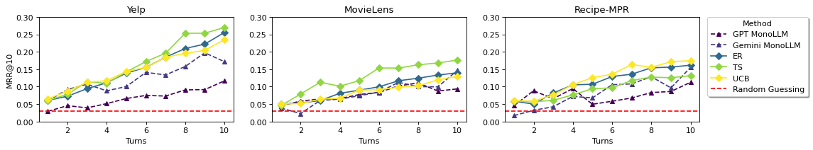
Figure 4 shows MRR@10 over 10 dialogue turns for MonoLLM and PEBOL (UCB,TS,ER),101010For each PEBOL policy, we use the MNLI temperature that performed best on the most datasets with continuous responses (see Supplementary Materials). with 95% confidence intervals (CIs) at turn 10 shown in Figure 8 (see Supplementary Materials for CIs for all turns and experiments). All methods start near random guessing, reflecting a cold start, and show clear preference learning over time.
Compared to GPT-MonoLLM, which uses the same LLM (GPT-3.5-turbo-0613) as PEBOL does for query generation, after 10 turns of dialogue PEBOL achieves: a mean MRR@10 of 0.27 vs. GPT-MonoLLM’s MRR@10 of 0.12 on Yelp; 0.18 vs 0.09 on MovieLens; and 0.17 vs 0.11 on Recipe-MPR, respectively. Compared to Gemini-MonoLLM, which uses a newer generation LLM (Gemini-Pro) than PEBOL for query generation, after 10 turns PEBOL still achieves a higher mean MRR@10 of 0.27 vs. Gemini-MonoLLM’s mean MRR@10 of 0.17 on Yelp; 0.18 vs. 0.15 on MovieLens, and 0.17 vs 0.16 on Recipe-MPR, respectively. While we did not have the resources to test PEBOL with Gemini query generation, we hypothesize that using a newer LLM for query generation can further improve PEBOL performance, since using the newer LLM (Gemini) shows performance improvements for the MonoLLM baseline.
6.2. RQ2 - Binary vs. Probabilistic Responses
Figure 6 compares PEBOL performance using binary (PEBOL-B) vs. continuous (PEBOL-P) feedback, and shows that performance is typically better when continuous responses are used – indicating that binary feedback models discard valuable information from the entailment probabilities.
6.3. RQ3 - Effect of User Response Noise
Figure 8 shows the impact of user response noise on MRR@10 at turn 10 – PEBOL generally continues to outperform MonoLLM under user response noise. Specifically, at all noise levels, both MonoLLM baselines are outperformed by all PEBOL-P variants on Yelp, and by at least one PEBOL-P variant on MovieLens and Recipe-MPR.
6.4. RQ4 - Comparison of Context Acquisition Policies
Figure 5 compares the performance of various PEBOL context acquisition policies – all policies show active preference learning, other than random item selection on RecipeMPR. There is considerable overlap between methods, however for most turns TS does well on Yelp and MovieLens while being beaten by Greedy, ER, and UCB on Recipe-MPR. As expected due to the randomness in sampling, TS performance is correlated with random item selection, while UCB performs quite similarly to greedy.
6.5. RQ5 - Effect of Aspect History in Query Generation
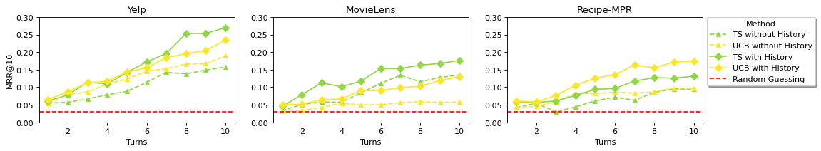
As shown in Figure 7, we see improvements in PEBOL performance from including a list of previously generated aspects in the aspect generation prompt. For instance, the differences in mean MRR@10 from including vs. excluding the query history for TS after 10 turns were: 0.27 vs 0.16 for Yelp; 0.18 vs 0.14 for MovieLens, and 0.13 vs 0.09 for Recipe-MPR, respectively. Practically, including the aspect generation history also helps to avoid repeat queries, which gain no information and could frustrate a user.
7. Conclusion and Future Work
This paper presents a novel Bayesian optimization formalization of natural language (NL) preference elicitation (PE) over arbitrary NL item descriptions, as well as introducing and evaluating PEBOL, an algorithm for NL Preference Elicitation with Bayesian Optimization augmented LLMs. As discussed below, our study also presents many opportunities for future work, including for addressing some of the limitations of PEBOL and our experiment setup.
User Studies
Firstly, our experiments limited by their reliance on LLM-simulated users. While the dialogue simulations indicate reasonable behaviour in the observed results, such as initial recommendation performance near random guessing, preference learning over time, and coherent user responses in logs such as those shown in Figure 7, future work would benefit from human user studies.
Multi-Item Belief Updates
While the assumption that item utilities can be updated independently allows the use of a simple and interpertable Beta-Bernouilli update model for each item, it also requires a separate NLI calculation to be performed for each item, which is computationally expensive. A key future direction is thus to explore alternative belief state forms which enable the joint updating of beliefs over all items from a single NLI computation.
Collaborative Belief Updates
Since PEBOL does not leverage any historical interactions with other users, an important future direction is to study NL-PE which leverages collaborative, multi-user data. One possibility is to initialize a cold start user’s prior beliefs based on interaction histories with other users. Another direction is adapting collaborative filtering based belief updating, such as the methods used in item-based feedback PE techniques (e.g., (Christakopoulou et al., 2016)), to NL-PE.
Diverse Query Forms
While PEBOL uses a pointwise query generation strategy that selects one item description at a time for LLM context, future work can explore LLM-based acquisition functions with pairwise and setwise context selection. Such multi-item context selection would enable contrastive query generation that could better discriminate between item preferences.
NL-PE in ConvRec Architectures
Another direction for future research is the integration of NL-PE methodologies such as PEBOL into conversational recommendation (ConvRec) system architectures (e.g., (Friedman et al., 2023; Kemper et al., 2024; Deldjoo et al., 2024; Korikov et al., 2024b)), which must balance many tasks including recommendation, explanation, and personalized question answering. Thus, in contrast to PEBOL’s pointwise queries and “yes-or-no” user responses, the use of PE in ConvRec systems implies that future algorithms will need to elicit preferences based on arbitrary pairs of NL system-user utterances. In these potential extensions, aspect-based NLI could be enabled by extracting aspects from utterances with LLMs (Korikov et al., 2024a).
References
- (1)
- Biyik et al. (2023) Erdem Biyik, Fan Yao, Yinlam Chow, Alex Haig, Chih-wei Hsu, Mohammad Ghavamzadeh, and Craig Boutilier. 2023. Preference Elicitation with Soft Attributes in Interactive Recommendation. ArXiv abs/2311.02085 (2023). https://api.semanticscholar.org/CorpusID:265034238
- Boutilier (2002) Craig Boutilier. 2002. A POMDP formulation of preference elicitation problems. In AAAI/IAAI. Edmonton, AB, 239–246.
- Brochu et al. (2010) Eric Brochu, Tyson Brochu, and Nando De Freitas. 2010. A Bayesian interactive optimization approach to procedural animation design. In Proceedings of the 2010 ACM SIGGRAPH/Eurographics Symposium on Computer Animation. 103–112.
- Chen et al. (2019) Qibin Chen, Junyang Lin, Yichang Zhang, Ming Ding, Yukuo Cen, Hongxia Yang, and Jie Tang. 2019. Towards Knowledge-Based Recommender Dialog System. In Proceedings of the 2019 Conference on Empirical Methods in Natural Language Processing and the 9th International Joint Conference on Natural Language Processing (EMNLP-IJCNLP), Kentaro Inui, Jing Jiang, Vincent Ng, and Xiaojun Wan (Eds.). Association for Computational Linguistics, Hong Kong, China, 1803–1813. https://doi.org/10.18653/v1/D19-1189
- Christakopoulou et al. (2016) Konstantina Christakopoulou, Filip Radlinski, and Katja Hofmann. 2016. Towards Conversational Recommender Systems. In Proceedings of the 22nd ACM SIGKDD International Conference on Knowledge Discovery and Data Mining (San Francisco, California, USA) (KDD ’16). Association for Computing Machinery, New York, NY, USA, 815–824.
- Dagan et al. (2005) Ido Dagan, Oren Glickman, and Bernardo Magnini. 2005. The PASCAL recognising textual entailment challenge. In Machine Learning Challenges Workshop. Springer, 177–190.
- Deldjoo et al. (2024) Yashar Deldjoo, Zhankui He, Julian McAuley, Anton Korikov, Scott Sanner, Arnau Ramisa, René Vidal, Maheswaran Sathiamoorthy, Atoosa Kasirzadeh, and Silvia Milano. 2024. A Review of Modern Recommender Systems Using Generative Models (Gen-RecSys). In Proceedings of the 30th ACM SIGKDD Conference on Knowledge Discovery and Data Mining (KDD ’24), August 25–29, 2024, Barcelona, Spain.
- Eric et al. (2007) Brochu Eric, Nando Freitas, and Abhijeet Ghosh. 2007. Active preference learning with discrete choice data. Advances in Neural Information Processing Systems 20 (2007).
- Friedman et al. (2023) Luke Friedman, Sameer Ahuja, David Allen, Terry Tan, Hakim Sidahmed, Changbo Long, Jun Xie, Gabriel Schubiner, Ajay Patel, Harsh Lara, et al. 2023. Leveraging Large Language Models in Conversational Recommender Systems. arXiv preprint arXiv:2305.07961 (2023).
- Garnett (2023) Roman Garnett. 2023. Bayesian optimization. Cambridge University Press.
- González et al. (2017) Javier González, Zhenwen Dai, Andreas Damianou, and Neil D Lawrence. 2017. Preferential bayesian optimization. In International Conference on Machine Learning. PMLR, 1282–1291.
- Guo and Sanner (2010) Shengbo Guo and Scott Sanner. 2010. Real-time multiattribute Bayesian preference elicitation with pairwise comparison queries. In Proceedings of the Thirteenth International Conference on Artificial Intelligence and Statistics. JMLR Workshop and Conference Proceedings, 289–296.
- Guo et al. (2010) Shengbo Guo, Scott Sanner, and Edwin V Bonilla. 2010. Gaussian process preference elicitation. Advances in Neural Information Processing Systems 23 (2010).
- Handa et al. (2024) Kunal Handa, Yarin Gal, Ellie Pavlick, Noah Goodman, Jacob Andreas, Alex Tamkin, and Belinda Z. Li. 2024. Bayesian Preference Elicitation with Language Models. arXiv:2403.05534 [cs.CL]
- He et al. (2023) Zhankui He, Zhouhang Xie, Rahul Jha, Harald Steck, Dawen Liang, Yesu Feng, Bodhisattwa Prasad Majumder, Nathan Kallus, and Julian McAuley. 2023. Large Language Models as Zero-Shot Conversational Recommenders. Proceedings of the 32nd ACM International Conference on Information and Knowledge Management (2023).
- Karamanolakis et al. (2018) Giannis Karamanolakis, Kevin Raji Cherian, Ananth Ravi Narayan, Jie Yuan, Da Tang, and Tony Jebara. 2018. Item recommendation with variational autoencoders and heterogeneous priors. In Proceedings of the 3rd Workshop on Deep Learning for Recommender Systems. 10–14.
- Kemper et al. (2024) Sara Kemper, Justin Cui, Kai Dicarlantonio, Kathy Lin, Danjie Tang, Anton Korikov, and Scott Sanner. 2024. Retrieval-Augmented Conversational Recommendation with Prompt-based Semi-Structured Natural Language State Tracking. In Proceedings of the 47th International ACM SIGIR Conference on Research and Development in Information Retrieval (Washington, DC, USA) (SIGIR ’24). ACM, New York, NY, USA.
- Khajah et al. (2016) Mohammad M. Khajah, Brett D. Roads, Robert V. Lindsey, Yun-En Liu, and Michael C. Mozer. 2016. Designing Engaging Games Using Bayesian Optimization. In Proceedings of the 2016 CHI Conference on Human Factors in Computing Systems (San Jose, California, USA) (CHI ’16). Association for Computing Machinery, New York, NY, USA, 5571–5582. https://doi.org/10.1145/2858036.2858253
- Korikov et al. (2024a) Anton Korikov, George Saad, Ethan Baron, Mustafa Khan, Manav Shah, and Scott Sanner. 2024a. Multi-Aspect Reviewed-Item Retrieval via LLM Query Decomposition and Aspect Fusion. In Proceedings of the 1st SIGIR’24 Workshop on Information Retrieval’s Role in RAG Systems, July 18, 2024, Washington D.C., USA.
- Korikov et al. (2024b) Anton Korikov, Scott Sanner, Yashar Deldjoo, Francesco Ricci, Zhankui He, Julian McAuley, Arnau Ramisa, Rene Vidal, Maheswaran Sathiamoorthy, Atoosa Kasirzadeh, and Silvia Milano. 2024b. Large Language Model Driven Recommendation. arXiv preprint arXiv:2404.XXXXX (2024).
- Lee et al. (2019) Hoyeop Lee, Jinbae Im, Seongwon Jang, Hyunsouk Cho, and Sehee Chung. 2019. MeLU: Meta-Learned User Preference Estimator for Cold-Start Recommendation. In Proceedings of the 25th ACM SIGKDD International Conference on Knowledge Discovery & Data Mining (Anchorage, AK, USA) (KDD ’19). Association for Computing Machinery, New York, NY, USA, 1073–1082. https://doi.org/10.1145/3292500.3330859
- Lei et al. (2020) Wenqiang Lei, Gangyi Zhang, Xiangnan He, Yisong Miao, Xiang Wang, Liang Chen, and Tat-Seng Chua. 2020. Interactive Path Reasoning on Graph for Conversational Recommendation. In Proceedings of the 26th ACM SIGKDD International Conference on Knowledge Discovery & Data Mining (Virtual Event, CA, USA) (KDD ’20). Association for Computing Machinery, New York, NY, USA, 2073–2083. https://doi.org/10.1145/3394486.3403258
- Li et al. (2023) Belinda Z. Li, Alex Tamkin, Noah Goodman, and Jacob Andreas. 2023. Eliciting Human Preferences with Language Models. arXiv:2310.11589 [cs.CL]
- Li et al. (2010) Lihong Li, Wei Chu, John Langford, and Robert E Schapire. 2010. A contextual-bandit approach to personalized news article recommendation. In Proceedings of the 19th International Conference on World Wide Web. 661–670.
- Li et al. (2011) Lihong Li, Wei Chu, John Langford, and Xuanhui Wang. 2011. Unbiased offline evaluation of contextual-bandit-based news article recommendation algorithms. In Proceedings of the Fourth ACM International Conference on Web Search and Data Mining. 297–306.
- Li et al. (2018) Raymond Li, Samira Ebrahimi Kahou, Hannes Schulz, Vincent Michalski, Laurent Charlin, and Chris Pal. 2018. Towards deep conversational recommendations. Advances in Neural Information Processing Systems 31 (2018).
- Li et al. (2021) Shijun Li, Wenqiang Lei, Qingyun Wu, Xiangnan He, Peng Jiang, and Tat-Seng Chua. 2021. Seamlessly Unifying Attributes and Items: Conversational Recommendation for Cold-start Users. ACM Trans. Inf. Syst. 39, 4, Article 40 (aug 2021), 29 pages. https://doi.org/10.1145/3446427
- Maynez et al. (2020) Joshua Maynez, Shashi Narayan, Bernd Bohnet, and Ryan McDonald. 2020. On Faithfulness and Factuality in Abstractive Summarization. In Proceedings of the 58th Annual Meeting of the Association for Computational Linguistics, Dan Jurafsky, Joyce Chai, Natalie Schluter, and Joel Tetreault (Eds.). Association for Computational Linguistics, Online, 1906–1919. https://doi.org/10.18653/v1/2020.acl-main.173
- Rossi and Sperduti (2004) Francesca Rossi and Allesandro Sperduti. 2004. Acquiring both constraint and solution preferences in interactive constraint systems. Constraints 9, 4 (2004), 311–332.
- Shahriari et al. (2016) Bobak Shahriari, Kevin Swersky, Ziyu Wang, Ryan P. Adams, and Nando de Freitas. 2016. Taking the Human Out of the Loop: A Review of Bayesian Optimization. Proc. IEEE 104, 1 (2016), 148–175. https://doi.org/10.1109/JPROC.2015.2494218
- Thorne et al. (2018) James Thorne, Andreas Vlachos, Christos Christodoulopoulos, and Arpit Mittal. 2018. FEVER: a Large-scale Dataset for Fact Extraction and VERification. In Proceedings of the 2018 Conference of the North American Chapter of the Association for Computational Linguistics: Human Language Technologies, Volume 1 (Long Papers), Marilyn Walker, Heng Ji, and Amanda Stent (Eds.). Association for Computational Linguistics, New Orleans, Louisiana, 809–819. https://doi.org/10.18653/v1/N18-1074
- Vendrov et al. (2020) Ivan Vendrov, Tyler Lu, Qingqing Huang, and Craig Boutilier. 2020. Gradient-Based Optimization for Bayesian Preference Elicitation. Proceedings of the AAAI Conference on Artificial Intelligence 34, 06 (Apr. 2020), 10292–10301. https://doi.org/10.1609/aaai.v34i06.6592
- Wang et al. (2022) Xiaolei Wang, Kun Zhou, Ji-Rong Wen, and Wayne Xin Zhao. 2022. Towards unified conversational recommender systems via knowledge-enhanced prompt learning. In Proceedings of the 28th ACM SIGKDD Conference on Knowledge Discovery and Data Mining. 1929–1937.
- Williams et al. (2018) Adina Williams, Nikita Nangia, and Samuel Bowman. 2018. A Broad-Coverage Challenge Corpus for Sentence Understanding through Inference. In Proceedings of the 2018 Conference of the North American Chapter of the Association for Computational Linguistics: Human Language Technologies, Volume 1 (Long Papers) (New Orleans, Louisiana). Association for Computational Linguistics, 1112–1122. http://aclweb.org/anthology/N18-1101
- Yang et al. (2022) Bowen Yang, Cong Han, Yu Li, Lei Zuo, and Zhou Yu. 2022. Improving Conversational Recommendation Systems’ Quality with Context-Aware Item Meta-Information. In Findings of the Association for Computational Linguistics: NAACL 2022. 38–48.
- Yang et al. (2021) Hojin Yang, Scott Sanner, Ga Wu, and Jin Peng Zhou. 2021. Bayesian Preference Elicitation with Keyphrase-Item Coembeddings for Interactive Recommendation. In Proceedings of the 29th ACM Conference on User Modeling, Adaptation and Personalization. 55–64.
- Yin et al. (2019) Wenpeng Yin, Jamaal Hay, and Dan Roth. 2019. Benchmarking Zero-shot Text Classification: Datasets, Evaluation and Entailment Approach. In Proceedings of the 2019 Conference on Empirical Methods in Natural Language Processing and the 9th International Joint Conference on Natural Language Processing (EMNLP-IJCNLP), Kentaro Inui, Jing Jiang, Vincent Ng, and Xiaojun Wan (Eds.). Association for Computational Linguistics, Hong Kong, China, 3914–3923. https://doi.org/10.18653/v1/D19-1404
- Zhang et al. (2023) Haochen Zhang, Anton Korikov, Parsa Farinneya, Mohammad Mahdi Abdollah Pour, Manasa Bharadwaj, Ali Pesaranghader, Xi Yu Huang, Yi Xin Lok, Zhaoqi Wang, Nathan Jones, and Scott Sanner. 2023. Recipe-MPR: A Test Collection for Evaluating Multi-aspect Preference-based Natural Language Retrieval. In Proceedings of the 46th International ACM SIGIR Conference on Research and Development in Information Retrieval (Taipei, Taiwan) (SIGIR ’23). Association for Computing Machinery, New York, NY, USA, 2744–2753. https://doi.org/10.1145/3539618.3591880
- Zhang et al. (2020) Xiaoying Zhang, Hong Xie, Hang Li, and John C.S. Lui. 2020. Conversational Contextual Bandit: Algorithm and Application. In Proceedings of The Web Conference 2020 (Taipei, Taiwan) (WWW ’20). Association for Computing Machinery, New York, NY, USA, 662–672. https://doi.org/10.1145/3366423.3380148
- Zhao et al. (2013) Xiaoxue Zhao, Weinan Zhang, and Jun Wang. 2013. Interactive collaborative filtering. In Proceedings of the 22nd ACM International Conference on Information & Knowledge Management. 1411–1420.
Appendix A Probabilistic Graphical Model for Posterior Utility Update

In this section, we present the probabilistic graphical model for the posterior utility updates introduced in our paper with a more detailed derivation of the posterior utility belief. As discussed in the paper, the objective of posterior inference is to update the prior belief maintained over the utility of each item denoted by given the query , item description , and , the binary observation variable representing whether the item description entails the user’s response to the queried preference .
Figure 9 shows the graphical model representation of these variables. The presented query and the item description are observed (shaded), while the relevance of item to query is latent (unshaded) and denoted by and conditioned on the latent item utility . We observe whether the item “truly” entails (i.e., ) the user’s response to query (as determined by the NLI entailment probability if the item is relevant, i.e., ). The conditional probability distributions in this graphical model are formally defined as follows:
| (20) | ||||
| (21) | ||||
| (22) |
To further explain the rationale for Eq (22), we note that is the natural language entailment probability that item description entails the aspect queried in the user’s response to given that item is relevant (). This entailment probability is obtained from the NLI model, which produces the probability that the entailment is true, hence the reason why . If item is instead irrelevant () then we assume for simplicity that is the probability of the true entailment.111111We note that an alternative approach (not used here) could attempt to use NLI to determine the probability of an incorrect true entailment (or confusion) given that item is irrelevant (). That is, there is no inherent requirement for the two cases of Eq (22) to sum to 1 since is on the conditional side.
To obtain the posterior utility , we need to marginalize the joint distribution over . Formally,
| (23) |
Considering the conditional independencies determined from the graphical model, the joint distribution factorizes as
| (24) |
Next, we replace the probability distribution of each factor according to Equations (20), (21), (22) in (23), to obtain
| (25) |
Expanding the summation yields
| (26) |
The latter term represents a mixture of Beta distributions that is challenging to handle since multiple posterior updates would cause the number of components in the mixture to grow exponentially with the number of query observations , leading to substantial computational and memory complexity.
To address this issue, several methods have been proposed for approximating the posterior distribution to allow for tractable computations. In this work, we use the Assumed Density Filtering (ADF) approach, a technique widely used in Bayesian filtering and tracking problems to project a complex posterior to an assumed simpler form (often the same form as the prior to maintain a closed-form). In our case, we project the Beta mixture posterior to a single Beta in order to maintain a closed-form Beta approximation of the posterior update matching the form of the Beta prior in Eq (20).
To apply ADF, we assume a Beta distribution with parameters and for the posterior, and approximate the original mixture of Beta’s with this distribution by equating their first moments (i.e., their means):
| (27) | ||||
| (28) |
Equating the numerators yields
| (29) |
and replacing this in the equation of the denominators results in
| (30) |
Thus, the “mean matched” posterior is .
Matching two distributions by equating their first moments is a special case of a more general technique called “moment matching”, which is widely used to approximate a complex probability distribution with a simpler one by equating their moments. In our work, we adopted a special case of this approach by matching the first moments, which we refer to as “mean matching” of the distributions that we used for its simplicity and intuitive interpretation. However, this is only one of the possible solutions, and a complete moment matching derivation results in a slightly different solution.
With this “mean matching” derivation and current item posterior at step , we can now perform an incremental posterior update after at step given the probability that the item description entails preference query yielding the closed-form Beta posterior as used in PEBOL-P.
| Dataset | Item Description | Generated Aspect | Generated Query |
|---|---|---|---|
| MovieLens |
Movie Title: Meet John Doe (1941)
Genres: Comedy, Drama Tags: Christianity, Frank Capra, acting, anti-fascism, class issues, journalism, patriotic, pro american, thought provoking, AFI 100 (Cheers), BD-R, Barbara Stanwyck, Gary Cooper, baseball player, compare: This Is Our Land (2017), domain, funny, radio broadcast, reviewed in the NYer by Anthony Lanne (2018-04-30), suicide note |
patriotism | Are you interested in movies with patriotic themes? |
| classic | Do you enjoy classic movies? | ||
| Recipe-MPR | Spaghetti with mushrooms, onion, green pepper, chicken breasts, and alfredo sauce | alfredo sauce | Do you like alfredo sauce? |
| chicken breast | Do you like chicken breasts? | ||
| Yelp | name: Le Pain Quotidien categories: Restaurants, Bakeries, Breakfast & Brunch, Coffee & Tea, Food, Belgian, French | bakery | Do you like bakeries? |
| French pastries | Do you like French pastries? |


| Turn | 1 | 2 | 3 | 4 | 5 | 6 | 7 | 8 | 9 | 10 |
|---|---|---|---|---|---|---|---|---|---|---|
| Method | ||||||||||
| MonoLLM GPT Mean | 0.04 | 0.06 | 0.06 | 0.07 | 0.08 | 0.08 | 0.10 | 0.11 | 0.09 | 0.09 |
| MonoLLM GPT CI LB | 0.01 | 0.02 | 0.02 | 0.02 | 0.03 | 0.03 | 0.05 | 0.06 | 0.04 | 0.04 |
| MonoLLM GPT CI UB | 0.08 | 0.10 | 0.11 | 0.11 | 0.12 | 0.13 | 0.15 | 0.16 | 0.14 | 0.15 |
| MonoLLM Gemini Mean | 0.04 | 0.02 | 0.06 | 0.06 | 0.07 | 0.08 | 0.11 | 0.10 | 0.10 | 0.15 |
| MonoLLM Gemini CI LB | 0.01 | 0.01 | 0.02 | 0.03 | 0.04 | 0.05 | 0.07 | 0.05 | 0.06 | 0.09 |
| MonoLLM Gemini CI UB | 0.07 | 0.04 | 0.10 | 0.10 | 0.11 | 0.12 | 0.16 | 0.15 | 0.14 | 0.20 |
| ER Mean | 0.05 | 0.05 | 0.06 | 0.08 | 0.09 | 0.10 | 0.12 | 0.12 | 0.13 | 0.14 |
| ER CI LB | 0.01 | 0.02 | 0.03 | 0.04 | 0.05 | 0.05 | 0.06 | 0.07 | 0.07 | 0.08 |
| ER CI UB | 0.08 | 0.09 | 0.09 | 0.12 | 0.13 | 0.15 | 0.17 | 0.18 | 0.19 | 0.20 |
| Greedy Mean | 0.05 | 0.05 | 0.07 | 0.07 | 0.09 | 0.09 | 0.10 | 0.10 | 0.11 | 0.13 |
| Greedy CI LB | 0.02 | 0.02 | 0.03 | 0.03 | 0.05 | 0.04 | 0.05 | 0.05 | 0.06 | 0.07 |
| Greedy CI UB | 0.09 | 0.09 | 0.10 | 0.11 | 0.14 | 0.14 | 0.15 | 0.15 | 0.17 | 0.19 |
| Random Mean | 0.05 | 0.05 | 0.08 | 0.11 | 0.12 | 0.14 | 0.14 | 0.16 | 0.16 | 0.14 |
| Random CI LB | 0.01 | 0.02 | 0.04 | 0.05 | 0.06 | 0.08 | 0.08 | 0.09 | 0.09 | 0.09 |
| Random CI UB | 0.08 | 0.09 | 0.13 | 0.16 | 0.18 | 0.21 | 0.20 | 0.22 | 0.22 | 0.20 |
| TS Mean | 0.05 | 0.08 | 0.11 | 0.10 | 0.12 | 0.15 | 0.15 | 0.16 | 0.17 | 0.18 |
| TS CI LB | 0.01 | 0.03 | 0.06 | 0.05 | 0.06 | 0.09 | 0.09 | 0.10 | 0.10 | 0.11 |
| TS CI UB | 0.08 | 0.13 | 0.17 | 0.15 | 0.17 | 0.22 | 0.21 | 0.23 | 0.23 | 0.24 |
| UCB Mean | 0.05 | 0.05 | 0.06 | 0.07 | 0.09 | 0.09 | 0.10 | 0.10 | 0.12 | 0.13 |
| UCB CI LB | 0.02 | 0.02 | 0.03 | 0.03 | 0.05 | 0.04 | 0.05 | 0.05 | 0.06 | 0.07 |
| UCB CI UB | 0.09 | 0.09 | 0.10 | 0.10 | 0.13 | 0.14 | 0.15 | 0.15 | 0.17 | 0.19 |
| Turn | 1 | 2 | 3 | 4 | 5 | 6 | 7 | 8 | 9 | 10 |
|---|---|---|---|---|---|---|---|---|---|---|
| Method | ||||||||||
| MonoLLM GPT Mean | 0.05 | 0.09 | 0.07 | 0.09 | 0.05 | 0.06 | 0.07 | 0.08 | 0.09 | 0.11 |
| MonoLLM GPT CI LB | 0.01 | 0.05 | 0.03 | 0.05 | 0.02 | 0.02 | 0.03 | 0.04 | 0.04 | 0.06 |
| MonoLLM GPT CI UB | 0.08 | 0.13 | 0.10 | 0.14 | 0.08 | 0.10 | 0.11 | 0.13 | 0.13 | 0.17 |
| MonoLLM Gemini Mean | 0.02 | 0.03 | 0.04 | 0.07 | 0.07 | 0.11 | 0.11 | 0.13 | 0.10 | 0.16 |
| MonoLLM Gemini CI LB | 0.01 | 0.02 | 0.02 | 0.04 | 0.03 | 0.06 | 0.07 | 0.08 | 0.06 | 0.10 |
| MonoLLM Gemini CI UB | 0.03 | 0.05 | 0.07 | 0.10 | 0.10 | 0.15 | 0.15 | 0.18 | 0.13 | 0.21 |
| ER Mean | 0.06 | 0.05 | 0.08 | 0.11 | 0.11 | 0.13 | 0.14 | 0.15 | 0.16 | 0.16 |
| ER CI LB | 0.02 | 0.02 | 0.04 | 0.06 | 0.06 | 0.08 | 0.08 | 0.09 | 0.09 | 0.10 |
| ER CI UB | 0.10 | 0.08 | 0.13 | 0.16 | 0.16 | 0.18 | 0.19 | 0.22 | 0.22 | 0.22 |
| Greedy Mean | 0.06 | 0.06 | 0.07 | 0.10 | 0.11 | 0.13 | 0.15 | 0.15 | 0.16 | 0.17 |
| Greedy CI LB | 0.02 | 0.02 | 0.03 | 0.05 | 0.06 | 0.07 | 0.09 | 0.09 | 0.10 | 0.11 |
| Greedy CI UB | 0.10 | 0.09 | 0.11 | 0.15 | 0.17 | 0.18 | 0.21 | 0.21 | 0.23 | 0.24 |
| Random Mean | 0.05 | 0.03 | 0.03 | 0.03 | 0.04 | 0.04 | 0.05 | 0.06 | 0.07 | 0.07 |
| Random CI LB | 0.02 | 0.01 | 0.01 | 0.00 | 0.01 | 0.01 | 0.02 | 0.02 | 0.03 | 0.02 |
| Random CI UB | 0.08 | 0.06 | 0.06 | 0.05 | 0.06 | 0.07 | 0.08 | 0.10 | 0.11 | 0.11 |
| TS Mean | 0.06 | 0.06 | 0.06 | 0.08 | 0.09 | 0.10 | 0.12 | 0.13 | 0.13 | 0.13 |
| TS CI LB | 0.02 | 0.02 | 0.02 | 0.03 | 0.05 | 0.05 | 0.06 | 0.07 | 0.07 | 0.07 |
| TS CI UB | 0.10 | 0.09 | 0.10 | 0.12 | 0.14 | 0.14 | 0.17 | 0.19 | 0.18 | 0.19 |
| UCB Mean | 0.06 | 0.06 | 0.08 | 0.11 | 0.13 | 0.14 | 0.16 | 0.16 | 0.17 | 0.17 |
| UCB CI LB | 0.02 | 0.02 | 0.03 | 0.06 | 0.07 | 0.08 | 0.10 | 0.09 | 0.11 | 0.11 |
| UCB CI UB | 0.10 | 0.09 | 0.12 | 0.16 | 0.18 | 0.19 | 0.23 | 0.22 | 0.24 | 0.24 |
| Turn | 1 | 2 | 3 | 4 | 5 | 6 | 7 | 8 | 9 | 10 |
|---|---|---|---|---|---|---|---|---|---|---|
| Method | ||||||||||
| MonoLLM GPT Mean | 0.03 | 0.05 | 0.04 | 0.05 | 0.07 | 0.07 | 0.07 | 0.09 | 0.09 | 0.12 |
| MonoLLM GPT CI LB | 0.01 | 0.01 | 0.01 | 0.02 | 0.03 | 0.03 | 0.03 | 0.04 | 0.04 | 0.06 |
| MonoLLM GPT CI UB | 0.05 | 0.08 | 0.07 | 0.08 | 0.10 | 0.12 | 0.12 | 0.14 | 0.14 | 0.17 |
| MonoLLM Gemini Mean | 0.06 | 0.09 | 0.11 | 0.09 | 0.10 | 0.14 | 0.13 | 0.16 | 0.20 | 0.17 |
| MonoLLM Gemini CI LB | 0.02 | 0.05 | 0.06 | 0.05 | 0.06 | 0.08 | 0.09 | 0.10 | 0.14 | 0.12 |
| MonoLLM Gemini CI UB | 0.10 | 0.14 | 0.15 | 0.13 | 0.14 | 0.20 | 0.18 | 0.21 | 0.26 | 0.23 |
| ER Mean | 0.06 | 0.07 | 0.09 | 0.11 | 0.14 | 0.16 | 0.18 | 0.21 | 0.22 | 0.26 |
| ER CI LB | 0.03 | 0.03 | 0.05 | 0.06 | 0.08 | 0.09 | 0.12 | 0.14 | 0.15 | 0.18 |
| ER CI UB | 0.10 | 0.11 | 0.14 | 0.16 | 0.20 | 0.22 | 0.25 | 0.28 | 0.29 | 0.33 |
| Greedy Mean | 0.06 | 0.08 | 0.11 | 0.11 | 0.14 | 0.15 | 0.17 | 0.18 | 0.19 | 0.22 |
| Greedy CI LB | 0.03 | 0.04 | 0.06 | 0.07 | 0.08 | 0.09 | 0.10 | 0.12 | 0.13 | 0.16 |
| Greedy CI UB | 0.10 | 0.12 | 0.15 | 0.16 | 0.20 | 0.21 | 0.23 | 0.25 | 0.26 | 0.29 |
| Random Mean | 0.06 | 0.09 | 0.11 | 0.13 | 0.17 | 0.17 | 0.17 | 0.18 | 0.20 | 0.21 |
| Random CI LB | 0.03 | 0.04 | 0.06 | 0.08 | 0.11 | 0.11 | 0.11 | 0.12 | 0.13 | 0.15 |
| Random CI UB | 0.10 | 0.13 | 0.16 | 0.19 | 0.23 | 0.23 | 0.23 | 0.24 | 0.26 | 0.28 |
| TS Mean | 0.06 | 0.08 | 0.11 | 0.11 | 0.14 | 0.17 | 0.20 | 0.25 | 0.25 | 0.27 |
| TS CI LB | 0.03 | 0.04 | 0.06 | 0.07 | 0.09 | 0.11 | 0.13 | 0.18 | 0.18 | 0.20 |
| TS CI UB | 0.10 | 0.12 | 0.17 | 0.15 | 0.20 | 0.23 | 0.26 | 0.33 | 0.32 | 0.34 |
| UCB Mean | 0.07 | 0.09 | 0.11 | 0.12 | 0.14 | 0.16 | 0.18 | 0.20 | 0.20 | 0.23 |
| UCB CI LB | 0.03 | 0.05 | 0.06 | 0.07 | 0.08 | 0.09 | 0.12 | 0.13 | 0.14 | 0.16 |
| UCB CI UB | 0.10 | 0.13 | 0.16 | 0.17 | 0.20 | 0.22 | 0.25 | 0.26 | 0.27 | 0.30 |
| Turn | 1 | 2 | 3 | 4 | 5 | 6 | 7 | 8 | 9 | 10 |
|---|---|---|---|---|---|---|---|---|---|---|
| Method | ||||||||||
| TS Mean | 0.03 | 0.05 | 0.06 | 0.06 | 0.08 | 0.11 | 0.13 | 0.12 | 0.13 | 0.14 |
| TS CI LB | 0.01 | 0.02 | 0.02 | 0.02 | 0.04 | 0.06 | 0.08 | 0.06 | 0.07 | 0.08 |
| TS CI UB | 0.06 | 0.09 | 0.09 | 0.09 | 0.13 | 0.16 | 0.19 | 0.17 | 0.18 | 0.19 |
| UCB Mean | 0.03 | 0.03 | 0.04 | 0.05 | 0.05 | 0.05 | 0.06 | 0.06 | 0.06 | 0.06 |
| UCB CI LB | 0.01 | 0.01 | 0.02 | 0.02 | 0.02 | 0.02 | 0.02 | 0.02 | 0.02 | 0.02 |
| UCB CI UB | 0.05 | 0.06 | 0.07 | 0.09 | 0.08 | 0.08 | 0.09 | 0.10 | 0.09 | 0.09 |
| Turn | 1 | 2 | 3 | 4 | 5 | 6 | 7 | 8 | 9 | 10 |
|---|---|---|---|---|---|---|---|---|---|---|
| Method | ||||||||||
| TS Mean | 0.04 | 0.05 | 0.03 | 0.04 | 0.06 | 0.07 | 0.06 | 0.09 | 0.10 | 0.09 |
| TS CI LB | 0.01 | 0.02 | 0.01 | 0.01 | 0.03 | 0.03 | 0.03 | 0.04 | 0.05 | 0.05 |
| TS CI UB | 0.07 | 0.09 | 0.05 | 0.07 | 0.10 | 0.12 | 0.10 | 0.13 | 0.14 | 0.14 |
| UCB Mean | 0.04 | 0.05 | 0.06 | 0.08 | 0.08 | 0.09 | 0.08 | 0.09 | 0.10 | 0.10 |
| UCB CI LB | 0.01 | 0.01 | 0.02 | 0.04 | 0.04 | 0.04 | 0.04 | 0.04 | 0.05 | 0.05 |
| UCB CI UB | 0.07 | 0.08 | 0.09 | 0.12 | 0.12 | 0.13 | 0.12 | 0.13 | 0.14 | 0.14 |
| Turn | 1 | 2 | 3 | 4 | 5 | 6 | 7 | 8 | 9 | 10 |
|---|---|---|---|---|---|---|---|---|---|---|
| Method | ||||||||||
| TS Mean | 0.05 | 0.06 | 0.07 | 0.08 | 0.09 | 0.11 | 0.14 | 0.14 | 0.15 | 0.16 |
| TS CI LB | 0.02 | 0.02 | 0.03 | 0.04 | 0.05 | 0.06 | 0.09 | 0.08 | 0.09 | 0.10 |
| TS CI UB | 0.09 | 0.09 | 0.10 | 0.11 | 0.13 | 0.16 | 0.20 | 0.19 | 0.21 | 0.22 |
| UCB Mean | 0.05 | 0.08 | 0.09 | 0.11 | 0.12 | 0.15 | 0.15 | 0.17 | 0.17 | 0.19 |
| UCB CI LB | 0.02 | 0.04 | 0.05 | 0.06 | 0.07 | 0.09 | 0.10 | 0.11 | 0.11 | 0.13 |
| UCB CI UB | 0.09 | 0.12 | 0.13 | 0.16 | 0.17 | 0.20 | 0.21 | 0.22 | 0.22 | 0.25 |
| Turn | 1 | 2 | 3 | 4 | 5 | 6 | 7 | 8 | 9 | 10 |
|---|---|---|---|---|---|---|---|---|---|---|
| Method | ||||||||||
| ER Mean | 0.03 | 0.04 | 0.04 | 0.05 | 0.06 | 0.08 | 0.09 | 0.11 | 0.11 | 0.12 |
| ER CI LB | 0.01 | 0.01 | 0.01 | 0.02 | 0.03 | 0.04 | 0.04 | 0.06 | 0.07 | 0.07 |
| ER CI UB | 0.06 | 0.07 | 0.08 | 0.08 | 0.10 | 0.12 | 0.14 | 0.16 | 0.16 | 0.16 |
| Greedy Mean | 0.03 | 0.04 | 0.05 | 0.05 | 0.07 | 0.09 | 0.10 | 0.11 | 0.11 | 0.11 |
| Greedy CI LB | 0.01 | 0.01 | 0.02 | 0.02 | 0.03 | 0.05 | 0.05 | 0.06 | 0.07 | 0.07 |
| Greedy CI UB | 0.06 | 0.08 | 0.08 | 0.09 | 0.11 | 0.13 | 0.14 | 0.16 | 0.16 | 0.16 |
| Random Mean | 0.03 | 0.04 | 0.04 | 0.06 | 0.06 | 0.08 | 0.09 | 0.10 | 0.10 | 0.10 |
| Random CI LB | 0.01 | 0.01 | 0.01 | 0.03 | 0.03 | 0.04 | 0.05 | 0.06 | 0.06 | 0.06 |
| Random CI UB | 0.06 | 0.06 | 0.07 | 0.09 | 0.10 | 0.12 | 0.13 | 0.14 | 0.14 | 0.14 |
| TS Mean | 0.03 | 0.05 | 0.06 | 0.07 | 0.08 | 0.07 | 0.09 | 0.12 | 0.12 | 0.13 |
| TS CI LB | 0.01 | 0.02 | 0.02 | 0.03 | 0.03 | 0.03 | 0.04 | 0.07 | 0.07 | 0.07 |
| TS CI UB | 0.06 | 0.08 | 0.09 | 0.11 | 0.12 | 0.11 | 0.13 | 0.17 | 0.18 | 0.18 |
| UCB Mean | 0.03 | 0.04 | 0.05 | 0.05 | 0.06 | 0.08 | 0.09 | 0.10 | 0.11 | 0.11 |
| UCB CI LB | 0.01 | 0.01 | 0.02 | 0.02 | 0.03 | 0.04 | 0.05 | 0.06 | 0.06 | 0.06 |
| UCB CI UB | 0.06 | 0.07 | 0.08 | 0.08 | 0.09 | 0.13 | 0.14 | 0.15 | 0.15 | 0.15 |
| Turn | 1 | 2 | 3 | 4 | 5 | 6 | 7 | 8 | 9 | 10 |
|---|---|---|---|---|---|---|---|---|---|---|
| Method | ||||||||||
| ER Mean | 0.04 | 0.06 | 0.09 | 0.07 | 0.09 | 0.09 | 0.10 | 0.13 | 0.10 | 0.10 |
| ER CI LB | 0.00 | 0.02 | 0.05 | 0.03 | 0.04 | 0.04 | 0.05 | 0.07 | 0.05 | 0.05 |
| ER CI UB | 0.07 | 0.10 | 0.14 | 0.10 | 0.14 | 0.14 | 0.16 | 0.19 | 0.15 | 0.15 |
| Greedy Mean | 0.04 | 0.04 | 0.06 | 0.07 | 0.10 | 0.11 | 0.12 | 0.12 | 0.12 | 0.13 |
| Greedy CI LB | 0.00 | 0.01 | 0.02 | 0.03 | 0.05 | 0.06 | 0.06 | 0.06 | 0.06 | 0.07 |
| Greedy CI UB | 0.07 | 0.08 | 0.10 | 0.10 | 0.15 | 0.17 | 0.18 | 0.18 | 0.18 | 0.19 |
| Random Mean | 0.04 | 0.03 | 0.03 | 0.05 | 0.04 | 0.04 | 0.05 | 0.04 | 0.05 | 0.06 |
| Random CI LB | 0.00 | 0.00 | 0.01 | 0.01 | 0.01 | 0.01 | 0.01 | 0.01 | 0.02 | 0.02 |
| Random CI UB | 0.07 | 0.06 | 0.05 | 0.09 | 0.07 | 0.08 | 0.08 | 0.07 | 0.09 | 0.11 |
| TS Mean | 0.04 | 0.06 | 0.06 | 0.07 | 0.09 | 0.09 | 0.10 | 0.10 | 0.11 | 0.12 |
| TS CI LB | 0.00 | 0.02 | 0.02 | 0.03 | 0.05 | 0.04 | 0.05 | 0.05 | 0.06 | 0.06 |
| TS CI UB | 0.07 | 0.09 | 0.10 | 0.12 | 0.14 | 0.14 | 0.16 | 0.15 | 0.17 | 0.17 |
| UCB Mean | 0.04 | 0.05 | 0.07 | 0.07 | 0.09 | 0.11 | 0.12 | 0.12 | 0.13 | 0.13 |
| UCB CI LB | 0.00 | 0.02 | 0.03 | 0.03 | 0.04 | 0.05 | 0.06 | 0.07 | 0.07 | 0.08 |
| UCB CI UB | 0.07 | 0.08 | 0.11 | 0.11 | 0.14 | 0.16 | 0.17 | 0.18 | 0.18 | 0.19 |
| Turn | 1 | 2 | 3 | 4 | 5 | 6 | 7 | 8 | 9 | 10 |
|---|---|---|---|---|---|---|---|---|---|---|
| Method | ||||||||||
| ER Mean | 0.05 | 0.05 | 0.07 | 0.09 | 0.11 | 0.11 | 0.11 | 0.11 | 0.11 | 0.11 |
| ER CI LB | 0.02 | 0.02 | 0.04 | 0.05 | 0.07 | 0.07 | 0.07 | 0.06 | 0.06 | 0.06 |
| ER CI UB | 0.08 | 0.09 | 0.11 | 0.12 | 0.15 | 0.15 | 0.15 | 0.15 | 0.15 | 0.15 |
| Greedy Mean | 0.05 | 0.06 | 0.08 | 0.09 | 0.10 | 0.10 | 0.10 | 0.10 | 0.10 | 0.10 |
| Greedy CI LB | 0.02 | 0.02 | 0.04 | 0.05 | 0.06 | 0.06 | 0.06 | 0.06 | 0.06 | 0.06 |
| Greedy CI UB | 0.08 | 0.09 | 0.11 | 0.13 | 0.14 | 0.13 | 0.13 | 0.14 | 0.14 | 0.13 |
| Random Mean | 0.05 | 0.06 | 0.07 | 0.09 | 0.11 | 0.10 | 0.10 | 0.11 | 0.12 | 0.14 |
| Random CI LB | 0.02 | 0.03 | 0.03 | 0.05 | 0.06 | 0.06 | 0.06 | 0.07 | 0.07 | 0.09 |
| Random CI UB | 0.08 | 0.09 | 0.11 | 0.14 | 0.15 | 0.14 | 0.14 | 0.15 | 0.16 | 0.19 |
| TS Mean | 0.05 | 0.06 | 0.12 | 0.12 | 0.16 | 0.16 | 0.18 | 0.18 | 0.22 | 0.24 |
| TS CI LB | 0.02 | 0.02 | 0.07 | 0.07 | 0.10 | 0.10 | 0.12 | 0.12 | 0.15 | 0.17 |
| TS CI UB | 0.08 | 0.10 | 0.17 | 0.17 | 0.22 | 0.22 | 0.24 | 0.24 | 0.28 | 0.31 |
| UCB Mean | 0.05 | 0.06 | 0.08 | 0.10 | 0.10 | 0.10 | 0.10 | 0.10 | 0.10 | 0.10 |
| UCB CI LB | 0.02 | 0.02 | 0.04 | 0.06 | 0.06 | 0.06 | 0.06 | 0.06 | 0.06 | 0.06 |
| UCB CI UB | 0.08 | 0.09 | 0.12 | 0.13 | 0.14 | 0.14 | 0.14 | 0.14 | 0.14 | 0.13 |
| Noise Level | 0 | 0.25 | 0.5 |
|---|---|---|---|
| Method | |||
| MonoLLM GPT Mean | 0.09 | 0.07 | 0.04 |
| MonoLLM GPT CI LB | 0.04 | 0.03 | 0.01 |
| MonoLLM GPT CI UB | 0.15 | 0.10 | 0.07 |
| MonoLLM Gemini Mean | 0.15 | 0.06 | 0.03 |
| MonoLLM Gemini CI LB | 0.09 | 0.02 | 0.00 |
| MonoLLM Gemini CI UB | 0.20 | 0.09 | 0.05 |
| ER Mean | 0.14 | 0.09 | 0.06 |
| ER CI LB | 0.08 | 0.04 | 0.03 |
| ER CI UB | 0.20 | 0.14 | 0.10 |
| Greedy Mean | 0.13 | 0.09 | 0.06 |
| Greedy CI LB | 0.07 | 0.04 | 0.02 |
| Greedy CI UB | 0.19 | 0.14 | 0.10 |
| Random Mean | 0.14 | 0.09 | 0.07 |
| Random CI LB | 0.09 | 0.05 | 0.03 |
| Random CI UB | 0.20 | 0.13 | 0.11 |
| TS Mean | 0.18 | 0.07 | 0.06 |
| TS CI LB | 0.11 | 0.03 | 0.02 |
| TS CI UB | 0.24 | 0.10 | 0.10 |
| UCB Mean | 0.13 | 0.08 | 0.07 |
| UCB CI LB | 0.07 | 0.04 | 0.03 |
| UCB CI UB | 0.19 | 0.13 | 0.11 |
| Noise Level | 0 | 0.25 | 0.5 |
|---|---|---|---|
| Method | |||
| MonoLLM GPT Mean | 0.11 | 0.06 | 0.05 |
| MonoLLM GPT CI LB | 0.06 | 0.02 | 0.01 |
| MonoLLM GPT CI UB | 0.17 | 0.11 | 0.08 |
| MonoLLM Gemini Mean | 0.16 | 0.13 | 0.08 |
| MonoLLM Gemini CI LB | 0.10 | 0.07 | 0.03 |
| MonoLLM Gemini CI UB | 0.21 | 0.19 | 0.12 |
| ER Mean | 0.16 | 0.15 | 0.09 |
| ER CI LB | 0.10 | 0.09 | 0.04 |
| ER CI UB | 0.22 | 0.22 | 0.13 |
| Greedy Mean | 0.17 | 0.13 | 0.07 |
| Greedy CI LB | 0.11 | 0.07 | 0.03 |
| Greedy CI UB | 0.24 | 0.19 | 0.11 |
| Random Mean | 0.07 | 0.04 | 0.02 |
| Random CI LB | 0.02 | 0.01 | 0.01 |
| Random CI UB | 0.11 | 0.06 | 0.04 |
| TS Mean | 0.13 | 0.06 | 0.06 |
| TS CI LB | 0.07 | 0.03 | 0.02 |
| TS CI UB | 0.19 | 0.08 | 0.10 |
| UCB Mean | 0.17 | 0.13 | 0.08 |
| UCB CI LB | 0.11 | 0.08 | 0.04 |
| UCB CI UB | 0.24 | 0.19 | 0.12 |
| Noise Level | 0 | 0.25 | 0.5 |
|---|---|---|---|
| Method | |||
| MonoLLM GPT Mean | 0.12 | 0.08 | 0.05 |
| MonoLLM GPT CI LB | 0.06 | 0.03 | 0.01 |
| MonoLLM GPT CI UB | 0.17 | 0.13 | 0.09 |
| MonoLLM Gemini Mean | 0.17 | 0.09 | 0.07 |
| MonoLLM Gemini CI LB | 0.12 | 0.05 | 0.02 |
| MonoLLM Gemini CI UB | 0.23 | 0.14 | 0.11 |
| ER Mean | 0.26 | 0.14 | 0.07 |
| ER CI LB | 0.18 | 0.08 | 0.03 |
| ER CI UB | 0.33 | 0.19 | 0.11 |
| Greedy Mean | 0.22 | 0.14 | 0.08 |
| Greedy CI LB | 0.16 | 0.09 | 0.04 |
| Greedy CI UB | 0.29 | 0.19 | 0.11 |
| Random Mean | 0.21 | 0.14 | 0.10 |
| Random CI LB | 0.15 | 0.09 | 0.05 |
| Random CI UB | 0.28 | 0.19 | 0.14 |
| TS Mean | 0.27 | 0.14 | 0.12 |
| TS CI LB | 0.20 | 0.08 | 0.06 |
| TS CI UB | 0.34 | 0.20 | 0.17 |
| UCB Mean | 0.23 | 0.13 | 0.10 |
| UCB CI LB | 0.16 | 0.08 | 0.05 |
| UCB CI UB | 0.30 | 0.18 | 0.14 |