Bayesian Meta-Learning on Control Barrier Functions with Data from On-Board Sensors
Abstract
In this paper, we consider a way to safely navigate the robots in unknown environments using measurement data from sensory devices. The control barrier function (CBF) is one of the promising approaches to encode safety requirements of the system and the recent progress on learning-based approaches for CBF realizes online synthesis of CBF-based safe controllers with sensor measurements. However, the existing methods are inefficient in the sense that the trained CBF cannot be generalized to different environments and the re-synthesis of the controller is necessary when changes in the environment occur. Thus, this paper considers a way to learn CBF that can quickly adapt to a new environment with few amount of data by utilizing the currently developed Bayesian meta-learning framework. The proposed scheme realizes efficient online synthesis of the controller as shown in the simulation study and provides probabilistic safety guarantees on the resulting controller.
Index Terms:
Control barrier function, learning-based control, meta-learning.I Introduction
ENSURING safety while achieving certain tasks is a fundamental yet challenging problem that has drawn significant attention from researchers in the control and robotics communities over the past few decades. In the control community, such safety requirements are often handled by imposing corresponding state constraints on an optimal control problem. Model Predictive Control (MPC) [1] and control synthesis methods based on the certificate functions such as Control Lyapunov Function (CLF) and Control Barrier Function (CBF) [2, 3, 4] are notable examples of such a method. Desirable theoretical results for these methods such as feasibility, stability, and safety are offered for known system dynamics [1, 2, 3, 4] or noisy dynamics with known noise distribution [5, 6, 7].
The CBF is a prominent tool to impose forward invariance of a safe set in state space. If a dynamical system is control-affine, quadratic programming formulation called CBF-QP [4] is available, which can produce safe control inputs much faster than many other control methods including MPC, and enables real-time implementations for challenging applications such as autonomous vehicles [8] and bipedal locomotion [9]. However, the majority of the existing works presuppose the availability of a valid CBF that represents safe and unsafe regions in state space. This assumption, however, cannot be maintained if a robot is expected to operate autonomously in unknown or uncertain environments. In such situations, it is essential for a robotic system to automatically identify unsafe regions on the fly, employing data from sensory devices. Thus, in this paper, we consider a learning-based method for constructing a CBF based on online measurements obtained from onboard sensors such as LiDAR scanners.
In the previous studies regarding this line of the topic (e.g., [31, 32, 33]), the robotic system iteratively improves the prediction of the CBF by collecting online sensor measurements without any prior knowledge about the environment or learning task. However, in such cases, even a slight change in the environment necessitates a complete retraining process, which is inefficient and requires a substantial amount of data. To efficiently and effectively learn CBF, adapting it to a new environment with minimal or small amount of training data, we suggest implementing meta-learning [10, 11], a technique that allows an agent to learn how to learn, as opposed to creating it from scratch. During the meta-training process, the model parameters are trained with data collected from various different environments, aiming to learn common underlying knowledge or structure of the learning task. The parameters obtained through meta-learning are then utilized as initial parameters for the online phase in a new environment and updated with online measurements in the environment. In this paper, we specifically employ a learning scheme combining the recently developed Bayesian meta-learning method [12] which is equipped with probabilistic bounds on the prediction [13], and the Bayesian surface reconstruction method [14, 15, 16] that can learn the unsafe regions from noisy sensor measurements. With this method, we can learn CBF and synthesize a safe controller with few amount of data and provide a probabilistic guarantee on the resulting controller.
Related works on learning and CBF : Learning-based approaches for certificate functions such as CBF and CLF are one of the active research topics in the area of intersections between control and learning [17]. In the following, we summarize the recent progress in the topic of learning and CBF. The authors of the works [18, 19, 20, 21, 22, 23] used CBF for active safe learning of uncertain dynamics. The works [18, 19] consider machine learning approaches to safely reduce the model uncertainty and show the methods yield empirically good performances, while the Gaussian Process (GP) is also used in [20, 21, 22, 23] and rigorous theoretical results for safety requirements are offered under certain assumptions. CBF is also used in Imitation Learning (IL) and Reinforcement Learning (RL) [25, 26, 24] to account for safety concerns.
While the above studies assume a valid CBF is given and consider leveraging it to impose safety conditions, several previous studies also consider parameterizing CBF itself by Neural Network (NN) and learning it to be a valid barrier function [27, 28, 29, 30, 31, 32, 33]. The work [27] considers jointly learning NNs representing CBF and CLF as well as a control policy based on safe and unsafe samples. The method proposed in [28] considers recovering CBF from expert demonstrations and theoretically guarantees that the learned NN meets the CBF conditions under the Lipsitz continuity assumptions. In [31], GP is also used to synthesize CBF. The works most related to this paper are [32, 33] which propose ways to learn CBF with sensor measurements. In [32], Support Vector Machine (SVM) classifier representing CBF is trained with safe and unsafe samples constructed by using the LiDAR measurements. Similarly, the authors of the work [33] present a synthesis method using Signed Distance Function (SDF).
Related works on meta-learning and control : Meta-learning, also known as “learning to learn,” is a technique capable of learning from previous learning experiences or tasks in order to improve the efficiency of future learning [10]. Meta-learning has recently become increasingly popular in the control literature. In several previous studies such as [13, 34], meta-learning is used to learn system dynamics to enable quick adaptation to the changes in surrounding situations. In these works, the trained models are incorporated into MPC which requires relatively heavy online computation. Meta-learning is also used in policy learning in the context of adaptive control [35] and reinforcement learning [10, 36].
Contributions: Our contributions compared to the existing methods are threefold: First, compared to the methods that synthesize CBF with sensor measurements [31, 32, 33] which rely on traditional supervised learning, the proposed meta-learning scheme can effectively use past data collected from different environments and produce a prediction of CBF with few amount of data. Consequently, the resulting control scheme realizes less conservative control performance with few amount of data (small number of online CBF updates) as we see in the case study. Second, different from the previous NN-based CBF synthesis methods [27, 29, 30, 32, 33], our method can readily take into account uncertainty in data and calculate formal probabilistic bounds on CBF. Based on this, we provide a probabilistic safety guarantee on the proposed control scheme. Although the work [33] takes into account the prediction error in SDF, such an error bound is assumed to be given and actual computation is not provided. Third, the learned CBF can readily be incorporated into ordinary QP formulation which can be efficiently solved. Thus, our method can produce control input much faster than the previous methods regarding meta-learning and MPC such as [13, 34].
Notations: A continuous functions and are class and extended class function, respectively, if they are strictly increasing with and . is the -th quantile of the distribution with degrees of freedom. The maximum and minimum eigenvalues for any positive definite matrix are defined as and , respectively. For vector fields and a function , is the Lie derivatives of the function in the direction of .
II Problem Statement
Throughout this paper, we consider the following control affine system:
| (1) |
where and with and are the admissible system states and control inputs respectively. The functions and are continuously differentiable functions representing dynamics of a robotic system (e.g., ground vehicles or drones) equipped with sensors such as LiDAR. The state space is assumed to contain initially unknown obstacles and the outside of each obstacle is defined by the following:
| (2) |
where is a continuously differentiable function with unobserved latent variable that encodes the geometric information about an obstacle, e.g., the position and shape of an obstacle. We assume realizations of the variable, , are determined by samples from a probabilistic distribution and they are fixed during the control execution. For simplicity, the obstacles are chosen not to overlap with each other.
Our goal is to synthesize a controller that achieves a given task (e.g., goal-reaching task) without deviating from the safe region given initial state . Since the safe/unsafe regions are initially unknown, the robotic system needs to identify them based on the sensor measurements. A naive approach toward this end is to use supervised learning based on measurement data obtained under a pre-determined environment. However, in this case, the trained model cannot be generalized to different environments, and even slight changes in the environment necessitate a complete re-fitting of the model, which is not only inefficient but also demands a substantial amount of data. Thus, this paper considers a way to effectively use past data regarding the different environments sampled from the distribution to quickly learn safe/unsafe regions in a new environment and synthesize the safe controller with few amount of online data.
III CBF-CLF-QP
In this section, we first introduce the Zeroing Control Barrier Function (ZCBF) as a tool to enforce safety on the system (1). The following discussion is a summary of the works [2, 4]. In ZCBF, the safety is defined as the forward-invariance of a safe set which is defined by the super zero level set of a function , i.e., the system (1) is considered to be safe if holds for all when . Given an extended class function , the ZCBF is defined as follows.
Definition 1.
Let be the zero super level set of a continuously differentiable function . Then, the function is a zeroing control barrier function (ZCBF) for (1) on if there exists an extended class function such that, for all the following inequality holds.
| (3) |
We additionally define the set of control inputs that satisfy the CBF condition as follows:
If the function is a valid CBF for (1) on , the safety of the system (1) is guaranteed as the following theorem.
Theorem 1 ([4]).
In this paper, the control objectives, except for the safety requirements, are encoded through the control Lyapunov function (CLF) which is given in advance. With a class function , the definition of CLF is formally given as follows [2].
Definition 2.
A continuously differentiable function is a CLF if with equilibrium point and there exists a class function such that, for all the following inequality holds.
| (4) |
Given a CLF , we consider the set of all control inputs that satisfy (4) for a state as
If a function is CLF, the stability of the equilibrium point is guaranteed as the following theorem.
Theorem 2 ([3]).
Having CBF and CLF defined above, we can synthesize a controller satisfying CBF and CLF conditions (3) and (4) with quadratic programming (QP) as follows:
| (5a) | ||||
| (5b) | ||||
| (5c) | ||||
| (5d) | ||||
where is a positive definite matrix and is a tunable parameter for relaxing the CLF condition (5b). The relaxation of the CLF condition ensures the solvability of the QP. If the safety is defined by multiple CBFs, we can handle them by adding the corresponding CBF constraints to the optimization problem.
IV Bayesian Meta-Learning of CBF
In this section, we consider learning the safe region (2) based on the measurement data from sensor devices. To this end, we employ a technique based on the Gaussian process implicit surfaces (GPIS) [14, 15, 16] which is developed for non-parametric probabilistic reconstruction of object surfaces. Note that we consider the case of for a while, and the case of multiple obstacles is discussed later in the next section. In this paper, the implicit surfaces (IS) are defined by the distance from the surface of objects to a certain point in 2D or 3D space, and the inside and outside of the object surfaces are interpreted through the sign of the function as follows.
| (9) |
where , is a position in a 2D or 3D space and is the function that returns the minimum Euclidean distance between and surface of the obstacle corresponding to . Though this paper focuses on a 2D environment, our method can easily be extended to a 3D case. In GPIS, the function is estimated with the Gaussian process (GP), which enables us to deal with uncertainty arising from measurement noise and scarcity of data. The GP is estimated with a dataset , where is bounded -subgaussian noise and is the number of data.
In the following, we explain how to construct a dataset and apply Bayesian meta-learning to the training of .
IV-A Dataset Construction
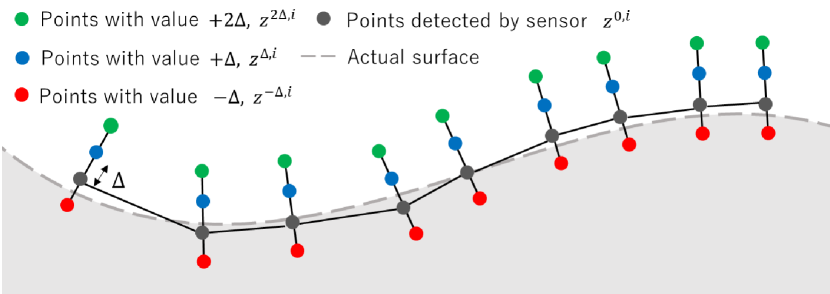
In this subsection, we explain how to construct a dataset to learn implicit surfaces (9) based on the measurement data from sensors such as LiDAR. A pictorial image for obtaining training data from noisy sensor measurements is shown in Fig. 1. First, assume we have a point cloud on the surface , where is the number of surface points and , are the world Cartesian coordinates of surface points computed with the raw depth readings produced by sensors and current position of the robot. Then, for each surface point , the normal to the surface of the obstacle at that point is approximated by the perpendicular to the segment between the point and the nearest neighbor point within the same scan [16]. Under the assumption that the sensor measurements on the surface are dense enough, this method yields accurate approximations. For each surface point and corresponding approximated normal to the surface, we construct a set of points with and , where , are the representations of the points that are away from the surface of the obstacle (see Fig 1). A negative value means that the point is inside the obstacle. Then, we construct the data set to train as .
IV-B Bayesian meta-learning of the function
When we train the IS function online, the efficiency of the training may be problematic while the model trained offline is not capable of generalizing to new environments. Thus, instead of relying on either online or offline training, we consider employing a meta-learning [10] scheme, which enables quick prediction on with a few amount of online data by effectively using data from different settings. In the following, we first introduce a Bayesian meta-learning framework ALPaCA (Adaptive Learning for Probabilistic Connectionist Architectures) [12]. Then, the probabilistic bounds on the prediction are subsequently discussed.
IV-B1 Overview of ALPaCA
We first parameterize the prediction of the function by the following form:
| (10) |
where represents a feed-forward neural network with parameter and is a coefficient matrix that follows a Gaussian distribution which encodes the information and uncertainty associated with the unknown variable . Here, denotes the mean parameters and is the positive definite precision matrix. Once the parameters of and the prior distribution, (), are determined through the offline meta-training procedure explained later, and the new measurement data along with a fixed is given as , the posterior distribution on is obtained as follows.
| (11) |
where , and . The above computation is based on Bayesian linear regression. Here, the mean and precision matrices are subscripted by to explicitly show that they are calculated using the data associated with unknown variable . Then, for any given , the mean and variance of the posterior predictive distribution are obtained as
| (12) |
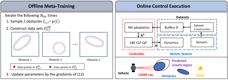
IV-B2 Offline meta-training procedures
In the offline meta-training procedure, the parameters (, , ) are trained so that the previously discussed online adaptation yields accurate prediction (The pseudo-code of the offline training is summarized in Algorithm 2 in Appendix -A). To this end, we iterate the following procedures prescribed times. First, we prepare data sets by sampling obstacles from the distribution and collect the data for each obstacle as , where is the number of data within . Then, we randomly split each dataset into training set and test set , where and are number of data within and with . In each iteration, is also randomly chosen from the uniform distribution over . The data within is used to calculate the posterior distribution on the parameter (i.e., mean and precision matrix ) through (11) while data within is used to evaluate the accuracy of the model (10) with the posterior parameters and calculated above. We define the meta-learning objective by the following marginal log-likelihood across the data and update the parameters through stochastic gradient descent.
| (13) |
IV-B3 Probabilistic bounds on CBF
From the discussions above, we can compute the predictive distribution of the function value for any and by (12) once the offline meta-training procedure discussed in Section IV-B2 has been done and new measurements are obtained along with the online execution. Here, we consider deriving a deterministic function with probabilistic guarantees, which can readily be incorporated in the QP formulation (5). The following discussion follows from [13]. Before deriving the probabilistic bounds on the prediction of , we make the following two assumptions on the quality of the offline meta-training, which are realistic and intuitive ones.
Assumption 1.
For all , there exists such that
| (14) |
Assumption 2.
For all , we have the following:
| (15) |
Assumption 1 implies that the meta-learning model (10) is capable of fitting the true function while Assumption 2 says that the uncertainty in the prior is conservative enough. Under these assumptions, we can derive the bounds on the function as follows.
Theorem 3.
Suppose the offline meta-training of the parameters , , and is done to satisfy Assumption 1 and 2, and the parameters defining posterior distribution and are computed by (11) with data from the new environment . Then, the L-1 norm of the difference between the true function value and the mean prediction with , for all and is bounded as the following.
| (16) |
with
with probability at least .
Proof.
Since the difference between the true value and mean prediction is bounded by , we can provide the lower bound of corresponding to a robot state as the following.
| (17) |
where is the function that maps the robot’s state to the robot’s position in 2D space. By using as the CBF, we can provide a probabilistic guarantee of the resulting controller as elaborated in Section V.
V Online Control Execution
Given system (1), meta-learned parameters , and CLF that encodes a control objective, the procedures in the online control execution is as summarized in Algorithm 1. Before the execution, an environment is determined by sampling the obstacles from the distribution and the data buffers for are initialized by empty sets (Line 1). Then, the control is executed by repeatedly solving the QP (5) with the CBFs (17) defined using the current posteriors and calculated by the data in the current buffers (Line 13,14). The buffers and the posterior parameters and are updated at every [s] through the procedures in the following subsection (Line 3-11). Since each buffer is empty at the beginning of the execution, we ignore the CBF constraint for until surface points of the corresponding obstacle are detected. To justify this, we make the following assumption.
Assumption 3.
The length of the laser is long enough and the measurements are taken constant enough such that the control invariant of the safe region is maintained even if the unobserved obstacles are ignored in the current QP.
In the following subsections, we discuss the update scheme of each buffer and the theoretical results of the proposed control scheme.
V-A The update scheme of each buffer
The update procedures of each buffer are discussed here. We ignore the subscription in the following discussion for simplicity of notation. At time instance , suppose we have new data points obtained by following the procedures in Section IV-A and the buffer which is constructed by the data points obtained at past time instances 0 to . Intuitively, the data points in will include many data points that are similar to those obtained in the past instances if the time interval of updating the dataset is small. Thus, it is important to select only the informative data points before adding them to the buffer. Here, we consider the data selection scheme for this purpose based on [39]. We repeat the following procedures for . First, we compute the predictive variance at a data point on the surface with posterior parameters calculated by the current as . Then, if the value is larger than the prescribed threshold , the data points are considered to be informative for the current model and thus added to the buffer .
V-B Theoretical Results
The probabilistic safety guarantees for our control scheme are summarized in the following theorem.
Theorem 4.
Proof.
From Theorem 1, the implicit control policy defined by the QP in Algorithm 1 keeps the system states within for all of the observed obstacles . Since each state in is included in the actual safe set with probability at least from Theorem 3, we can guarantee with probability at least for all and the observed obstacles . This result and Assumption 3 prove the theorem. ∎
VI Case Study
We test the proposed approach through a simulation of vehicle navigation in a 2D space. All the experiments are conducted on Python running on a Windows 10 with a 2.80 GHz Core i7 CPU and 32 GB of RAM. TensorFlow and PyBullet [38] are used for the meta-learning of the IS function and implementation of the vehicle system with LiDAR scanners, respectively. We define the controlled system by the unmanned vehicle that has the following dynamics:
| (18) |
where , , and are coordinates of the robot position and heading angle of the robot, and are the velocity and angular velocity of the vehicle, respectively. The control inputs and system states are defined as and , respectively. Note that in (18), we consider the dynamics of a point off the axis of the robot by a distance to make the system relative degree one [40]. Moreover, the LiDAR scanner which has a 360-degree field of view and radiates 150 rays with a 3-meter length is assumed to be mounted on the vehicle.
VI-A Meta learning of unsafe regions
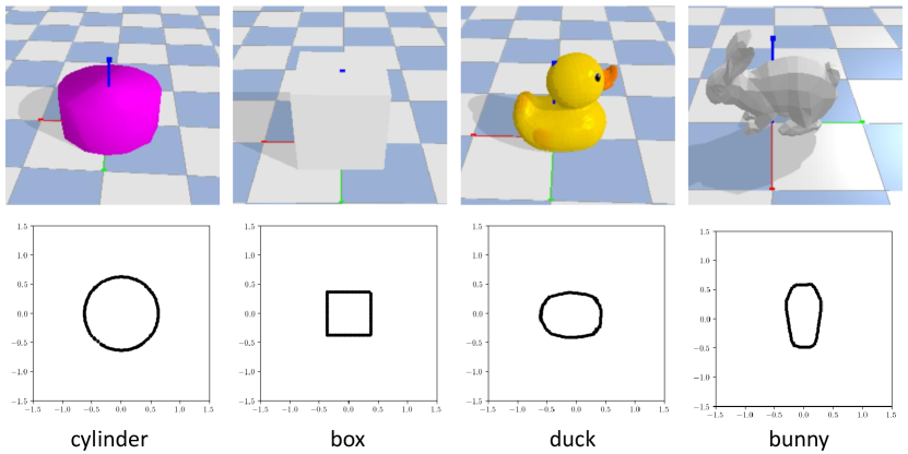
We first test the performance of the proposed scheme for constructing the IS function . We consider 2 settings: (I) ellipsoidal obstacles with randomly chosen semi-axes lengths, center positions, and rotation angles (II) Objects in Fig. 3 with randomly chosen positions, rotation angles, and scales. In setting (I), the IS function is defined by the ellipsoids as follows:
| (19) |
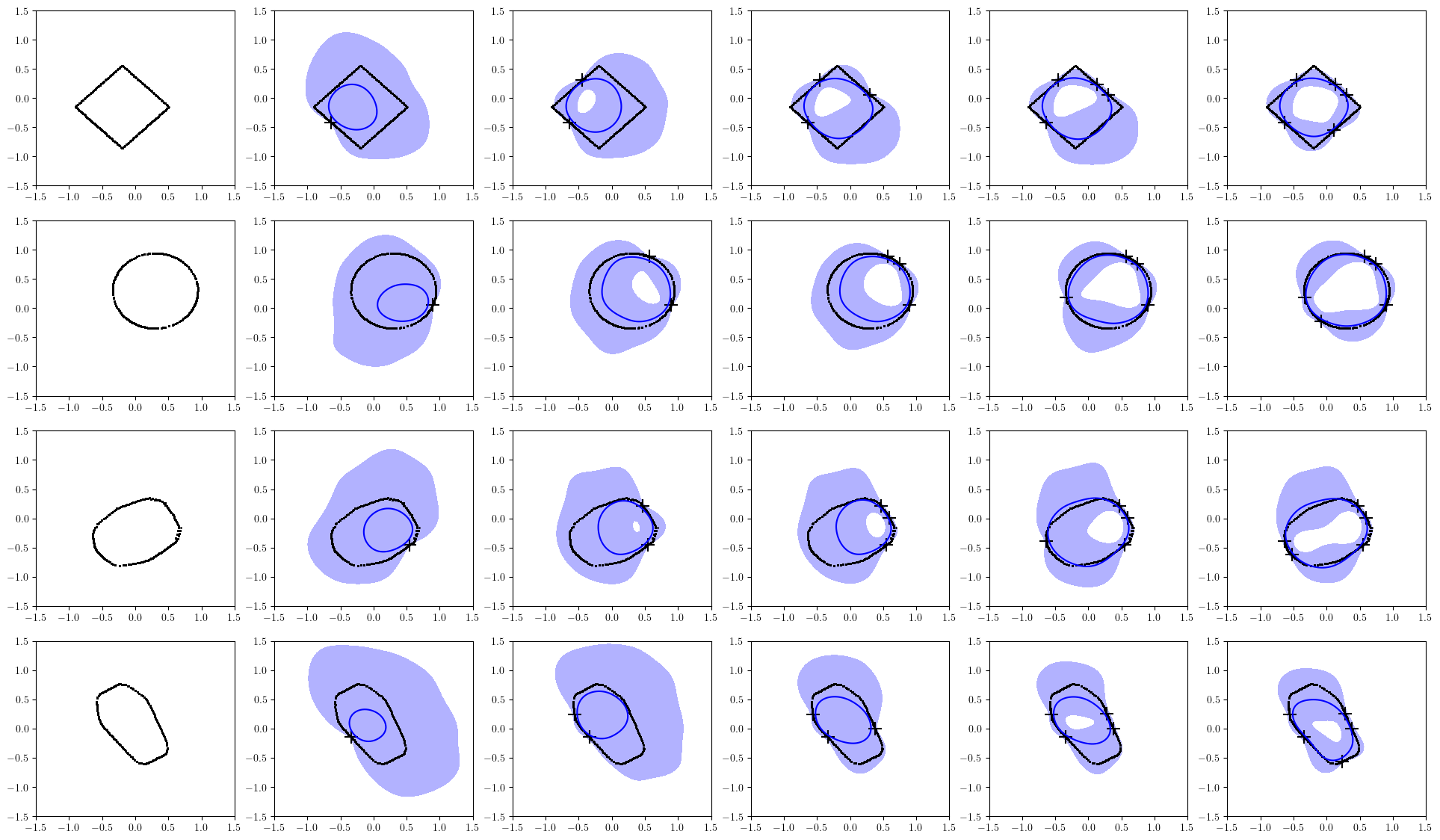
where , are the semi-axes lengths along the and coordinates respectively, is the rotation angle, is the center of the ellipsoid, and . In this example, the unobserved parameter can be explicitly written as . The parameters (, ), (, ), and are randomly sampled from the uniform distribution in the range , , and , respectively. In setting (II), we used object files in pybullet_data [41] to test with more arbitrary shapes. The rotational angles and the center position of the objects are sampled in the same way as setting (I). For both cases, the architecture of in (10) is defined by three hidden layers of 256 units with 32 basis functions. Moreover, we set , , , , and to 30000, 0.001, 1, 5, and 0.1, respectively.
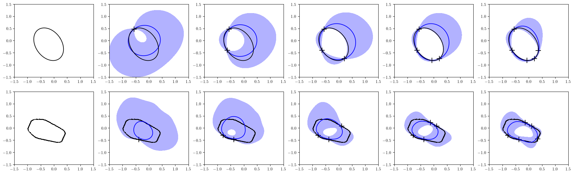
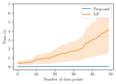
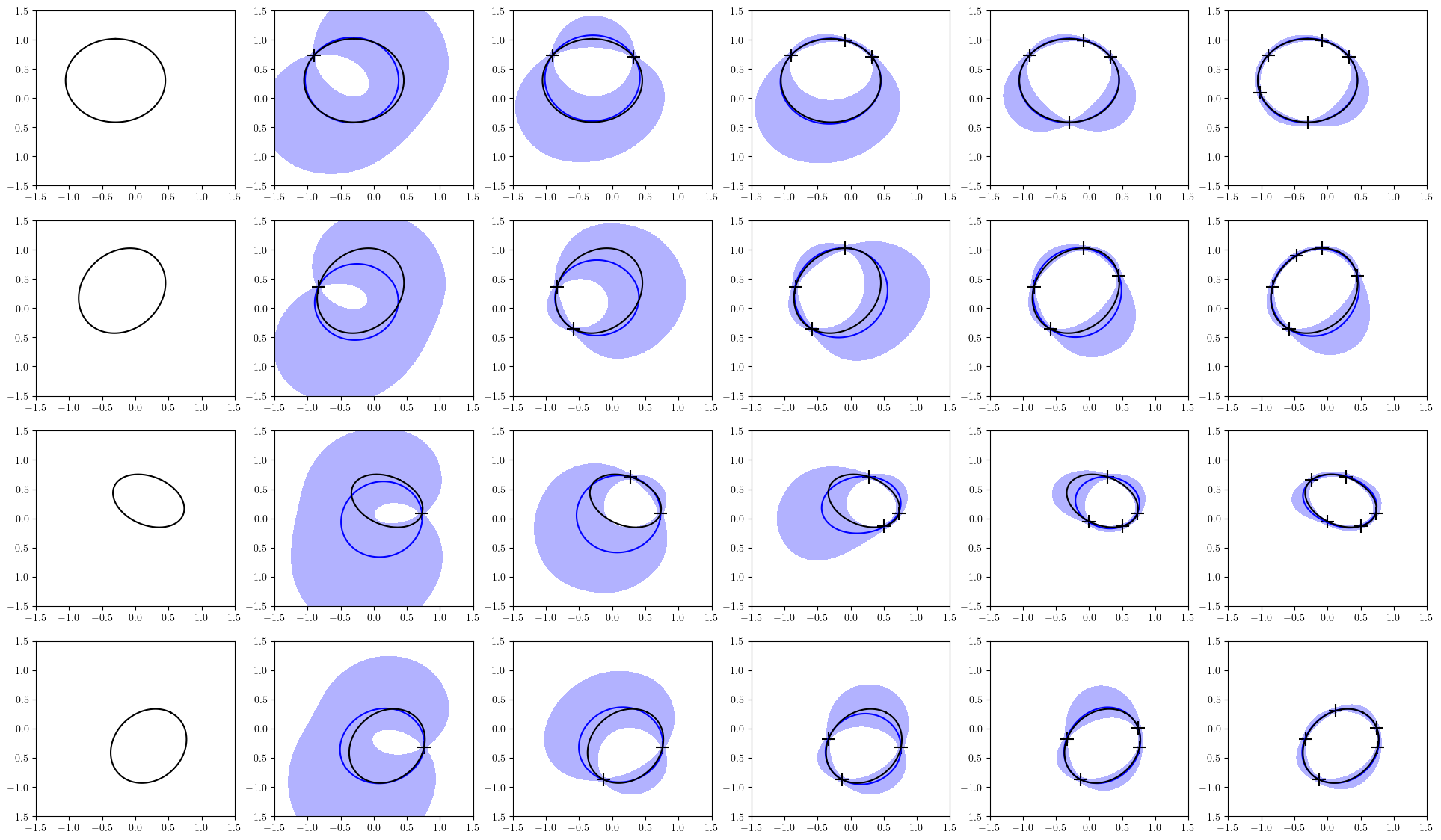
The prediction of an obstacle surface calculated with a small amount of data is shown in Figure 4. The blue lines and blue shaded areas in the figure are the mean predictions of the surfaces and the regions between the 0-level sets of the upper and lower 90% bounds of . We can see that the confidence bounds are reasonably tight even when the number of data points for the adaptation is small, which is the main effect of the offline meta-training. Moreover, same as reported in [12], the time required for the adaptation is much smaller than that of the GP [42] which is a commonly used Bayesian method. More results including the comparison to the GP in terms of both the accuracy of the prediction and time required for the training are provided in Appendix -C.
VI-B Control execution
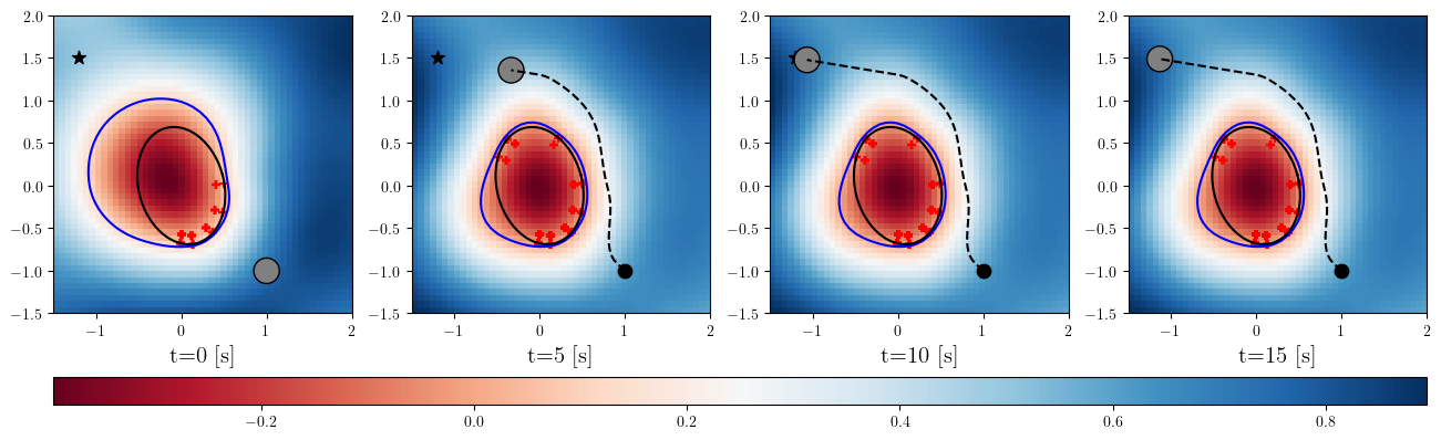
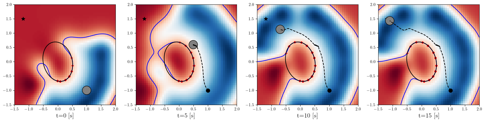
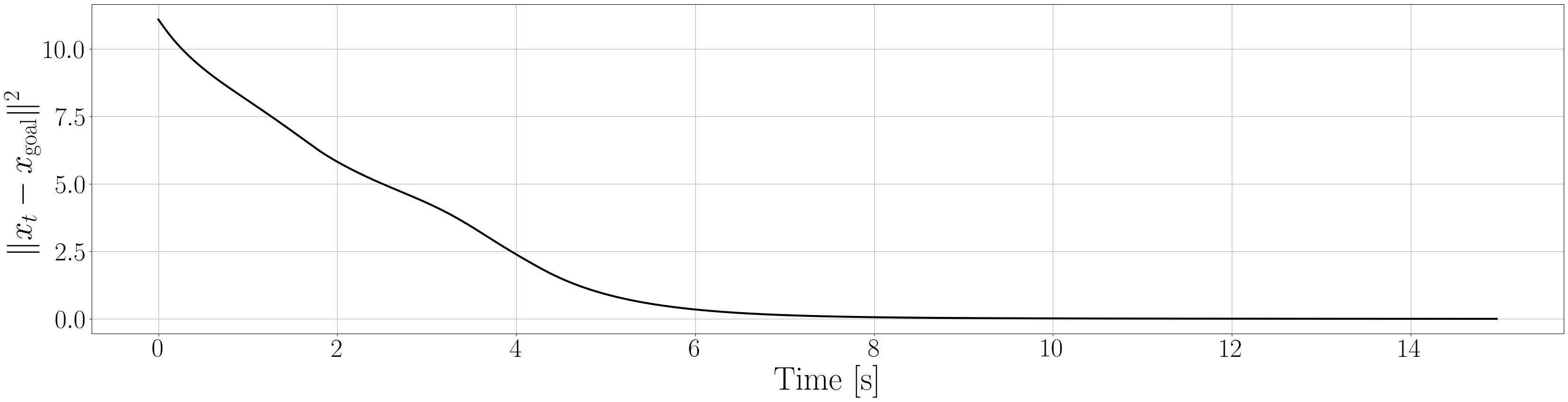
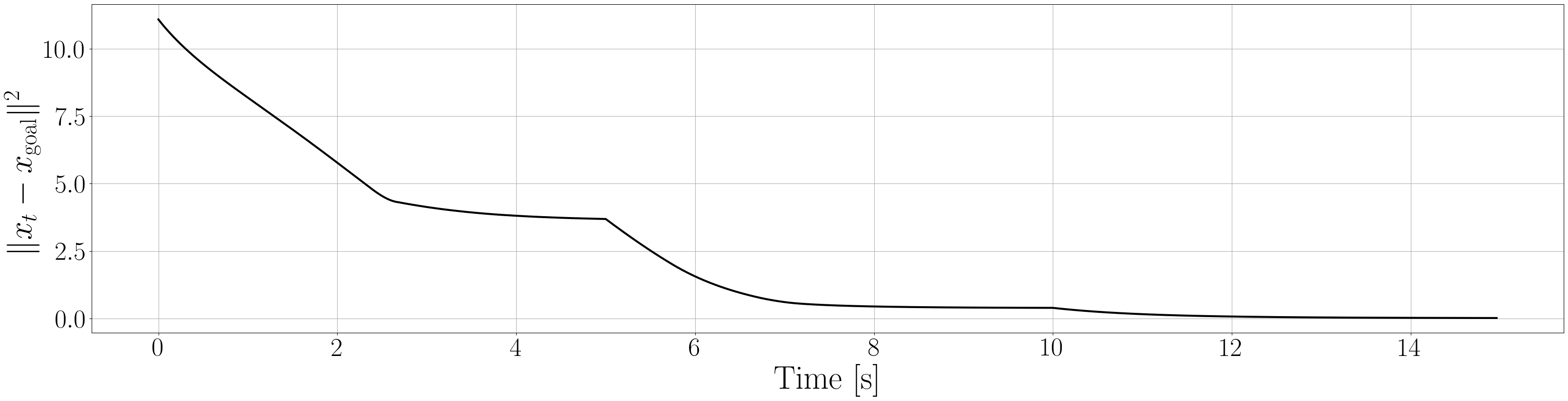
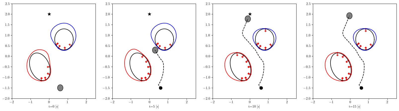
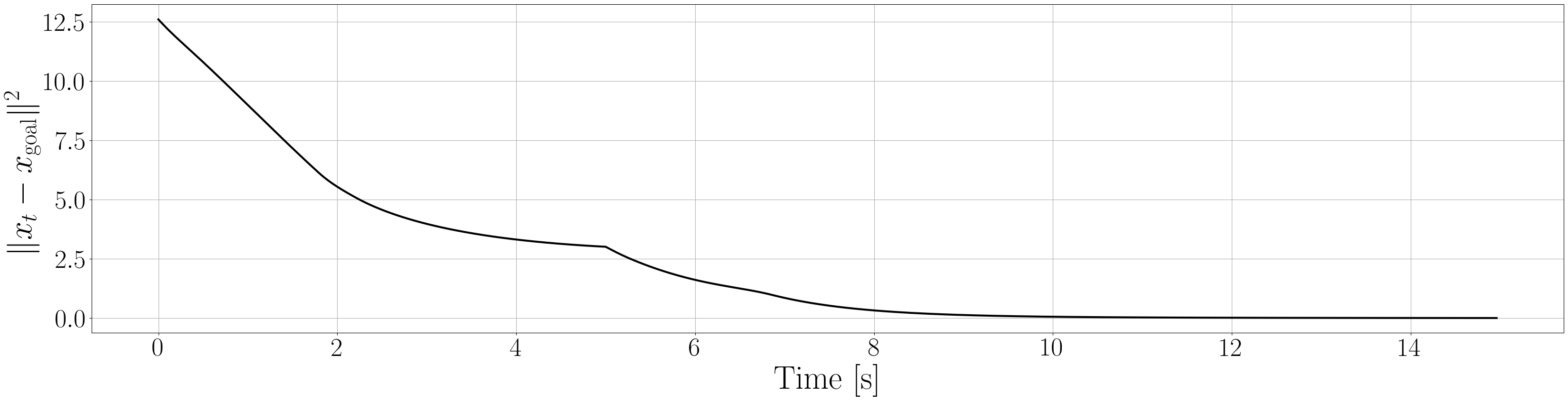
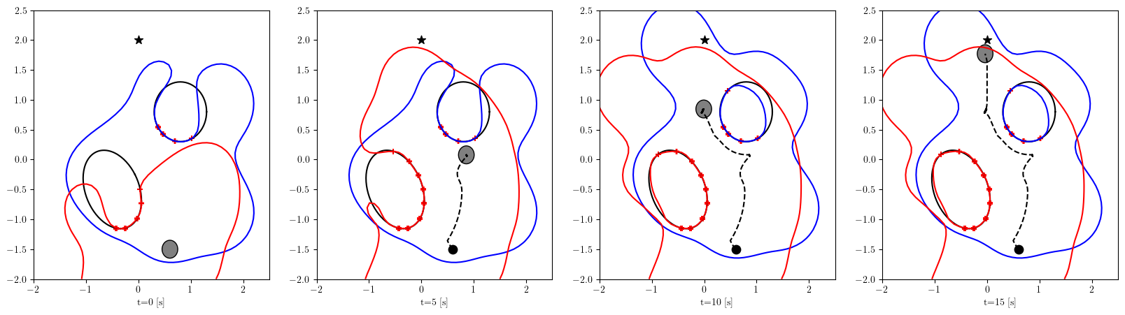
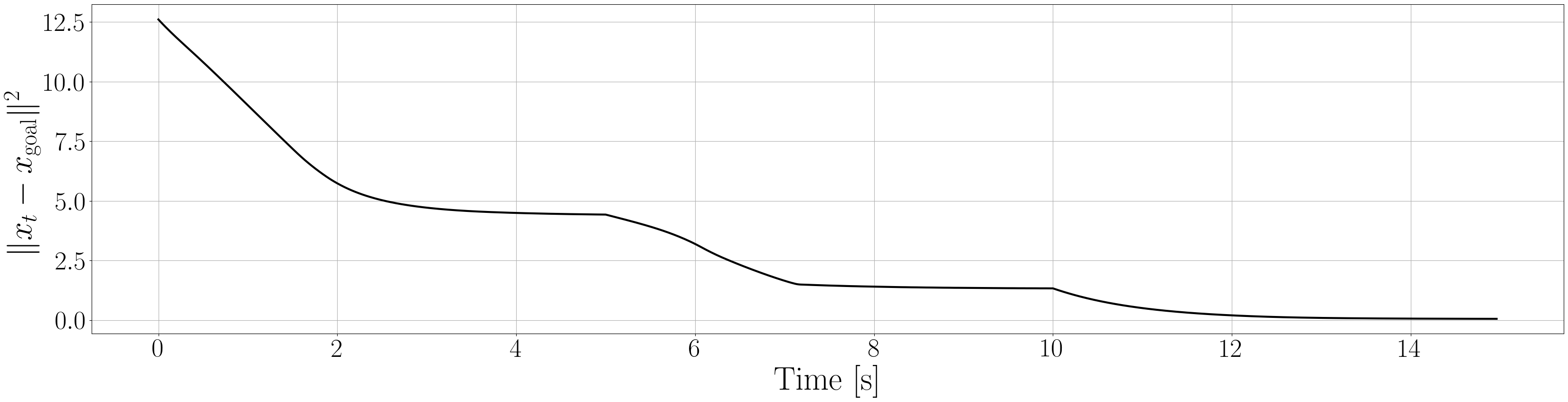
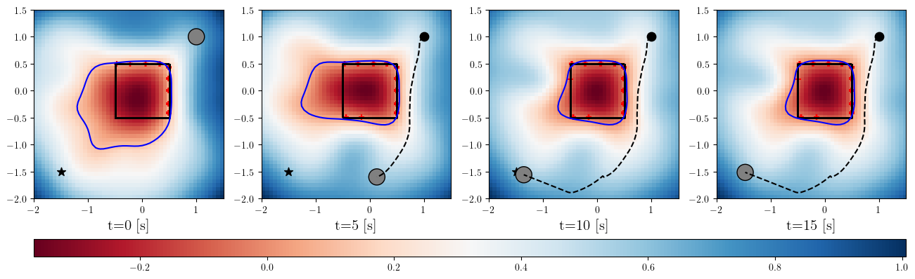
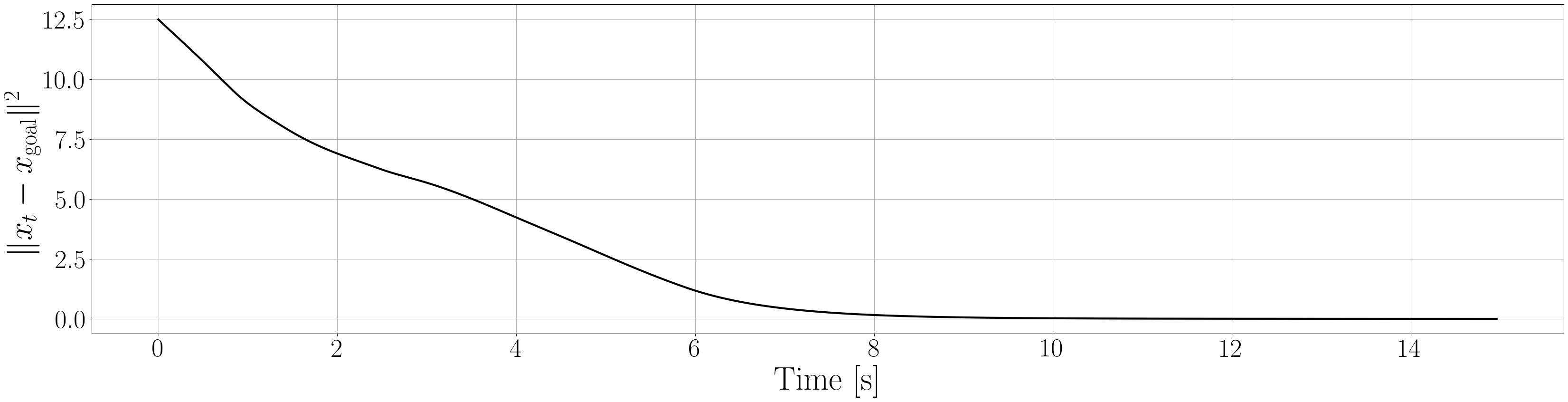
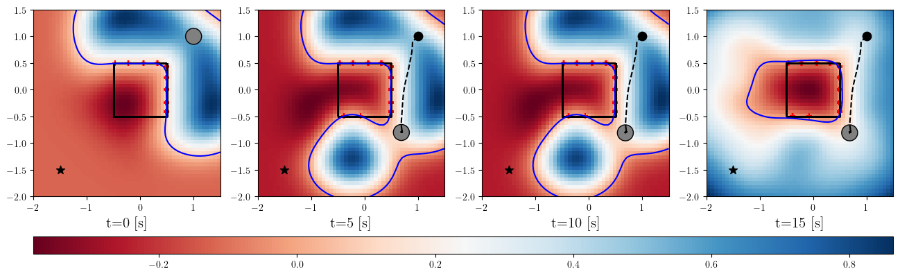
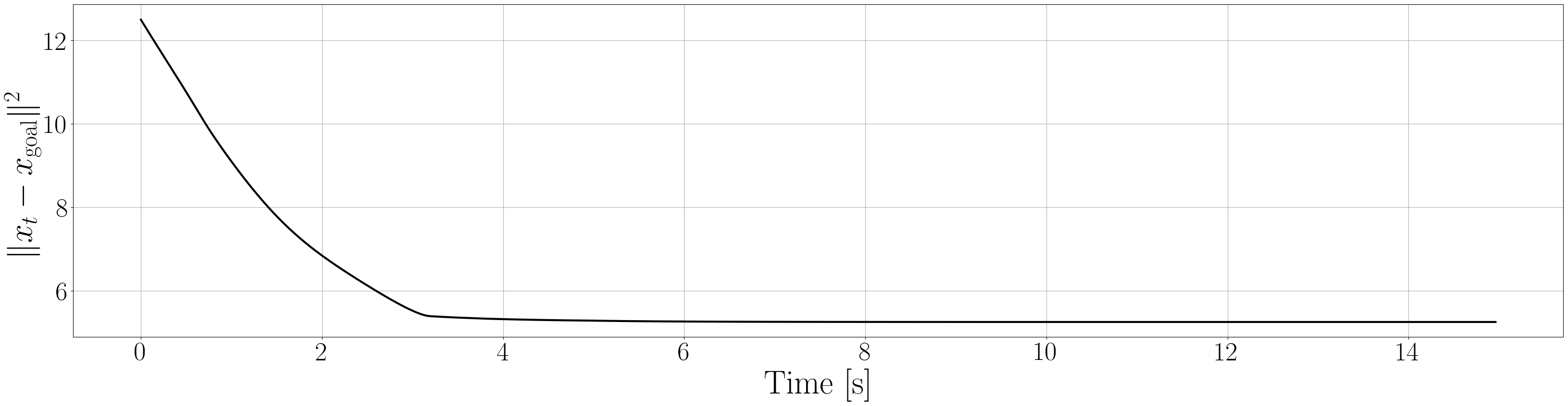
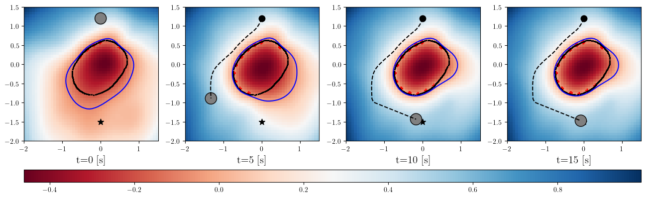
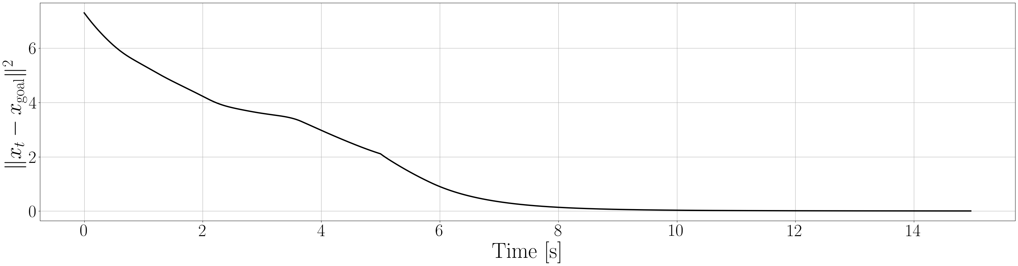
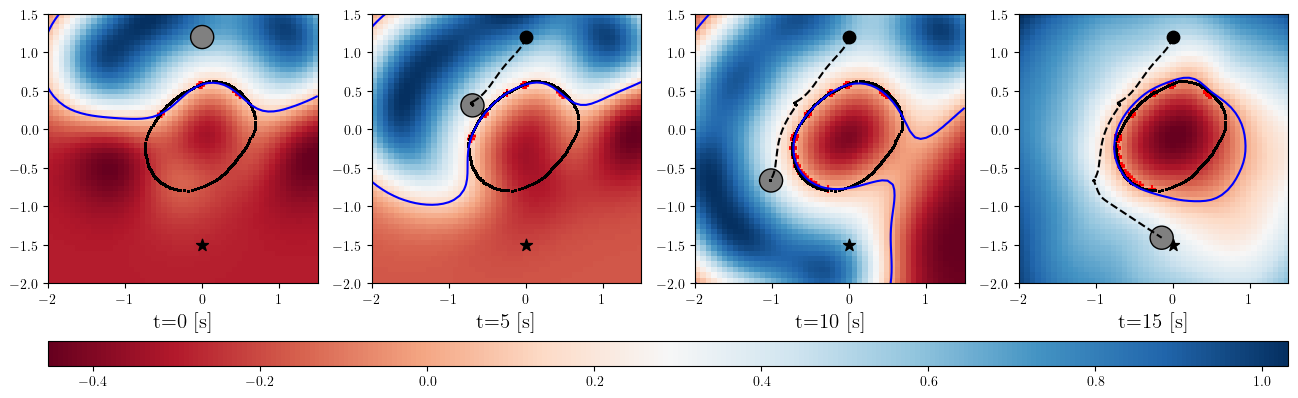
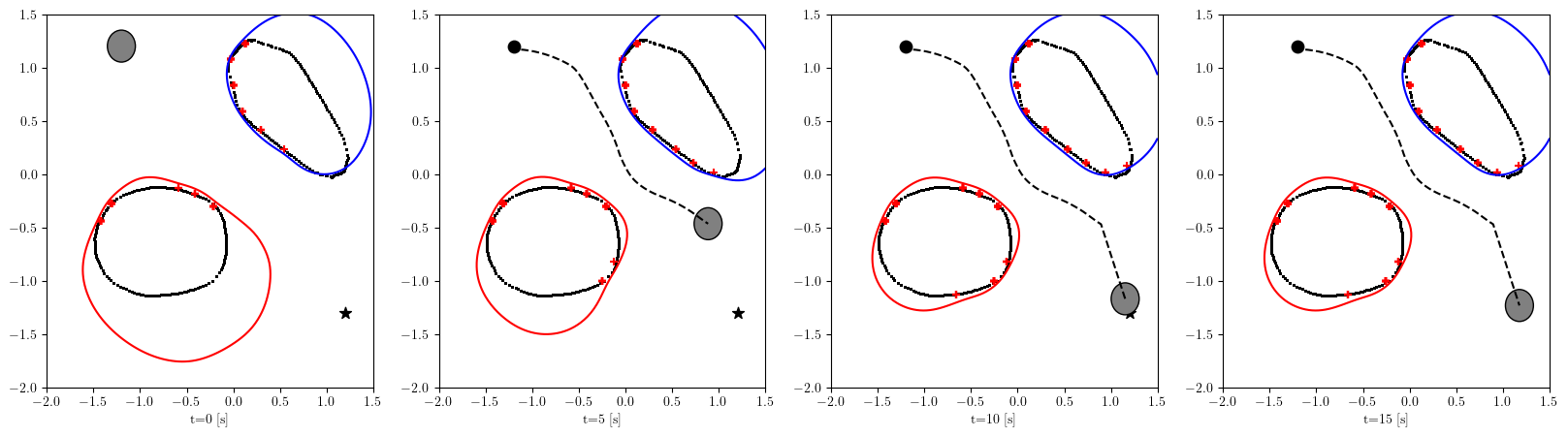
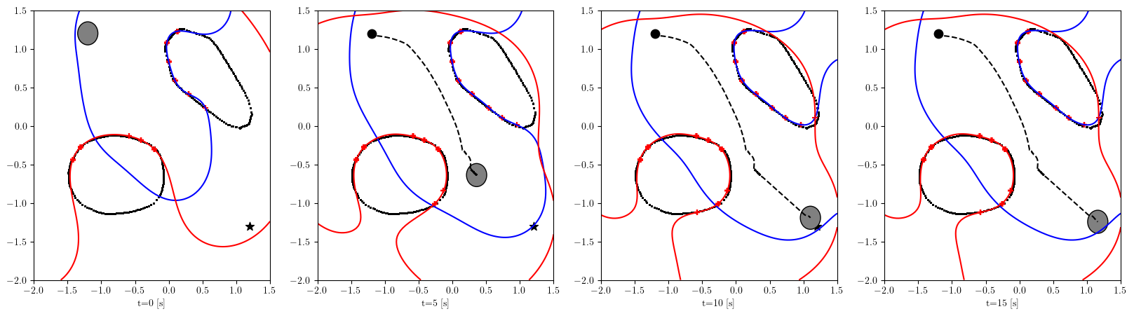
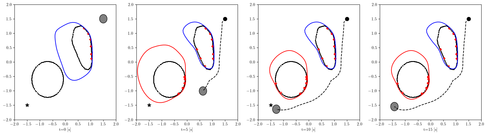
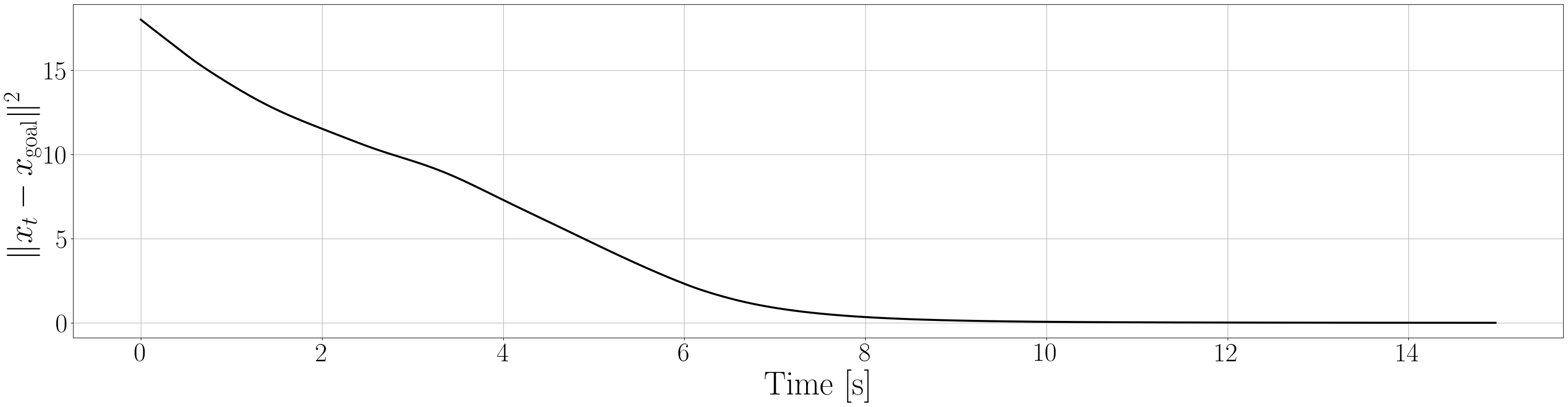
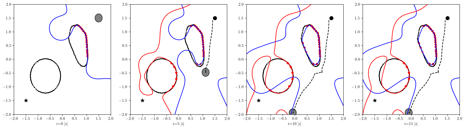
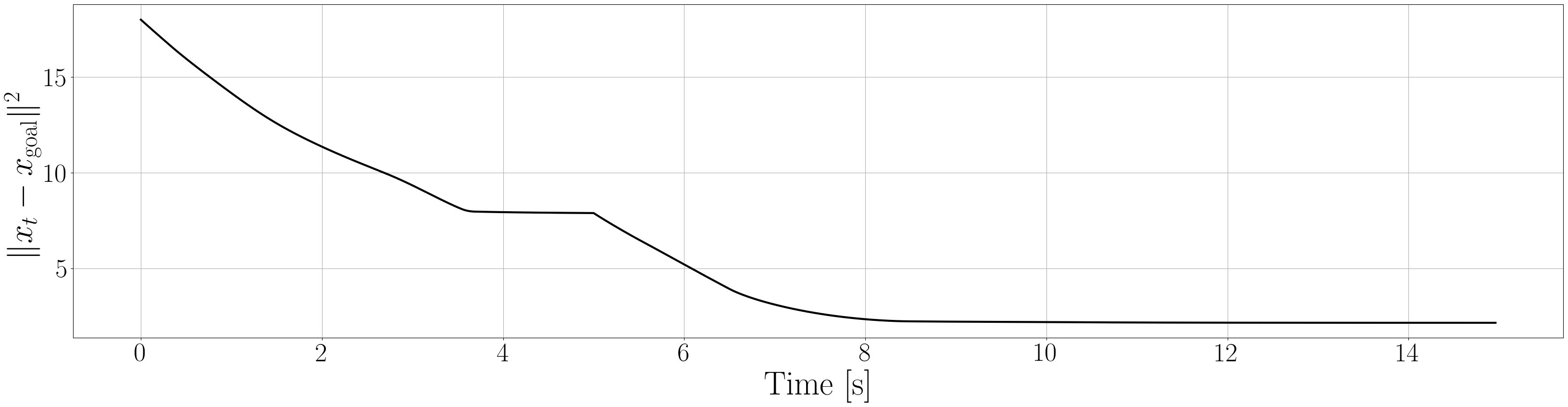
Based on the trained , we next consider executing the control with Algorithm 1. The control objective is to steer the vehicle toward the goal position while avoiding obstacles. The goal-reaching objective is encoded through the CLF . Moreover, and in (5) are defined by the linear functions and . We set parameters , , and to , , and 10, respectively. For comparison, we test the control performance of the proposed scheme and the case where the GP is used instead of ALPaCA. Since the theoretically guaranteed bounds of GP [43, 44] tend to be overly conservative, we instead use the 2- lower bounds in the GP case. The metric of the control performance is defined by the cumulative squared error (CSE) of the difference between the robot and goal positions, along with the resulting state trajectory (the squared errors are corrected every 0.02 [s]). An example of the control execution with [s] is visualized in Figure 5. From Figure 5, we can see the vehicle successfully reaches the goal while avoiding the unsafe region. Notably, the control of the proposed method is much less conservative than the GP case because of the tight prediction of the unsafe region (the vehicle in the GP case is often forced to be stacked in small safe regions until the subsequent update of the CBF). The CSEs in this case for the proposed method and GP case are 618 and 1010, respectively. We additionally provide results for different 5 environments with single or multiple obstacles in Appendix -D (the results for the cases are shown) and similar results are observed. Although the CSE of the proposed method and the GP case get closer as becomes smaller, it is ideal to maintain the value to be small to save computation and the use of sensor devices that have limited batteries. Moreover, the GP prediction can not be updated so frequently because of the time required for the training (see the time analysis in Appendix -C). From the results above, we can conclude that the proposed scheme has a practical advantage from the perspective of control.
VII Conclusion
In this paper, we proposed an efficient and probabilistically ensured online learning method of CBF with sensor measurements. In the proposed method, we utilized a technique based on the GPIS to train unsafe regions from the measurements. Specifically, a Bayesian meta-learning scheme was employed to learn IS function, which enables us to effectively use past data from different settings. To avoid the volume of data buffers becoming unnecessarily large in the online control execution, we also considered the data selection scheme which effectively uses the uncertainty information provided by the current model. The prediction made by the proposed scheme was readily incorporated in the CBF-CLF-QP formulation and the probabilistic safety guarantee for the control scheme was also provided. In the case study, we have shown the efficacy of our method in terms of the conservativeness of the prediction, the time required for the online training, and the conservativeness of the control performance.
References
- [1] E. F. Camacho and C. B. Alba, Model predictive control. Springer science & business media, 2013.
- [2] A. D. Ames, S. Coogan, M. Egerstedt, G. Notomista, K. Sreenath, and P. Tabuada, “Control barrier functions: Theory and applications,” in European Control Conference (ECC), 2019, pp. 3420–3431.
- [3] A. D. Ames, K. Galloway, K. Sreenath and J. W. Grizzle, “Rapidly Exponentially Stabilizing Control Lyapunov Functions and Hybrid Zero Dynamics,” in IEEE Transactions on Automatic Control, vol. 59, no. 4, pp. 876–891, 2014.
- [4] A. D. Ames, X. Xu, J. W. Grizzle and P. Tabuada, “Control Barrier Function Based Quadratic Programs for Safety Critical Systems,” in IEEE Transactions on Automatic Control, vol. 62, no. 8, pp. 3861–3876, 2017.
- [5] D. Q. Mayne, M. M. Seron, and S. Rakovic, “Robust model predictive ´ control of constrained linear systems with bounded disturbances,” Automatica, vol. 41, no. 2, pp. 219–224, 2005.
- [6] A. Clark, “Control Barrier Functions for Complete and Incomplete Information Stochastic Systems,” in American Control Conference (ACC), Philadelphia, 2019, pp. 2928-2935.
- [7] K. Garg and D. Panagou, “Robust Control Barrier and Control Lyapunov Functions with Fixed-Time Convergence Guarantees,” 2021 American Control Conference (ACC), 2021, pp. 2292-2297.
- [8] Y. Chen, H. Peng, and J. Grizzle, “Obstacle Avoidance for Low-Speed Autonomous Vehicles With Barrier Function,” in IEEE Transactions on Control Systems Technology, vol. 26, no. 1, pp. 194–206, 2018.
- [9] A. D. Ames, J. W. Grizzle, and P. Tabuada, “Control barrier function based quadratic programs with application to adaptive cruise control,” in IEEE Conference on Decision and Control, 2014, pp. 6271–6278.
- [10] C. Finn, P. Abbeel, and S. Levine, “Model-agnostic meta-learning for fast adaptation of deep networks,” in Proc. Int. Conf. Mach. Learn., 2017, pp. 1126–1135.
- [11] T. Hospedales, A. Antoniou, P. Micaelli and A. Storkey, “Meta-Learning in Neural Networks: A Survey,” in IEEE Transactions on Pattern Analysis and Machine Intelligence, vol. 44, no. 9, pp. 5149–5169, 2022.
- [12] J. Harrison, A. Sharma, and M. Pavone, “Meta-learning priors for efficient online Bayesian regression,” in Proc. Workshop Algorithmic Found. Robot., 2018, pp. 318–337.
- [13] T. Lew, A. Sharma, J. Harrison, A. Bylard and M. Pavone, ”Safe Active Dynamics Learning and Control: A Sequential Exploration–Exploitation Framework,” in IEEE Transactions on Robotics, vol. 38, no. 5, pp. 2888-2907, 2022.
- [14] O. Williams and A. Fitzgibbon, “Gaussian process implicit surfaces,” in Proc. Gaussian Process. Practice Workshop, 2007.
- [15] W. Martens, Y. Poffet, P. R. Soria, R. Fitch and S. Sukkarieh, “Geometric Priors for Gaussian Process Implicit Surfaces,” in IEEE Robotics and Automation Letters, vol. 2, no. 2, pp. 373–380, 2017.
- [16] M. Gerardo-Castro, T. Peynot, and F. Ramos, “Laser-radar data fusion with Gaussian process implicit surfaces,” in Proc. Field Serv. Robot., 2015, pp. 289–302.
- [17] C. Dawson, S. Gao, and C. Fan, “Safe Control with Learned Certificates: A Survey of Neural Lyapunov, Barrier, and Contraction methods,” in IEEE Transactions on Robotics, to be appeared, 2023.
- [18] A. Taylor, A. Singletary, Y. Yue, and A. Ames, “Learning for safety critical control with control barrier functions,” in Learning for Dynamics and Control, 2020, pp. 708–717.
- [19] J. Choi, F. Castaneda, C. Tomlin, and K. Sreenath, “Reinforcement ˜Learning for Safety-Critical Control under Model Uncertainty, using Control Lyapunov Functions and Control Barrier Functions,” in Robotics: Science and Systems, Corvalis, OR, 2020.
- [20] P. Jagtap, G. J. Pappas and M. Zamani, “Control Barrier Functions for Unknown Nonlinear Systems using Gaussian Processes,” in IEEE Conference on Decision and Control (CDC), 2020, pp. 3699–3704.
- [21] V. Dhiman, M. J. Khojasteh, M. Franceschetti and N. Atanasov, “Control Barriers in Bayesian Learning of System Dynamics,” in IEEE Transactions on Automatic Control, vol. 68, no. 1, pp. 214–229, 2023.
- [22] F. Castaneda, J. J. Choi, W. Jung, B. Zhang, C. J. Tomlin, and K. Sreenath, “Probabilistic Safe Online Learning with Control Barrier Functions,” arXiv:2208.10733, 2022.
- [23] K. Long, V. Dhiman, M. Leok, J. Cortés and N. Atanasov, ”Safe Control Synthesis With Uncertain Dynamics and Constraints,” in IEEE Robotics and Automation Letters, vol. 7, no. 3, pp. 7295-7302, July 2022
- [24] R. Cheng, G. Orosz, R. M. Murray, and J. W. Burdick, “End-to-end safe reinforcement learning through barrier functions for safety-critical continuous control tasks,” in AAAI Conference on Artificial Intelligence, vol. 33, 2019, pp. 3387–3395.
- [25] R. K. Cosner, Y. Yue and A. D. Ames, “End-to-End Imitation Learning with Safety Guarantees using Control Barrier Functions,” in IEEE Conference on Decision and Control (CDC), 2022, pp. 5316–5322.
- [26] S. Yaghoubi, G. Fainekos and S. Sankaranarayanan, “Training Neural Network Controllers Using Control Barrier Functions in the Presence of Disturbances,” in IEEE International Conference on Intelligent Transportation Systems (ITSC), 2020, pp. 1–6.
- [27] W. Jin, Z. Wang, Z. Yang, and S. Mou, “Neural Certificates for Safe Control Policies,” arXiv:2006.08465, 2020.
- [28] A. Robey, H. Hu, L. Lindemann, H. Zhang, D. V. Dimarogonas, S. Tu, and N. Matni, “Learning Control Barrier Functions from Expert Demonstrations,” in IEEE Conference on Decision and Control (CDC), 2020, pp. 3717–3724.
- [29] C. Dawson, Z. Qin, S. Gao, and C. Fan, “Safe Nonlinear Control Using Robust Neural Lyapunov-Barrier Functions,” in Proceedings of the 5th Conference on Robot Learning, vol. 164, 2022, pp. 1724–1735.
- [30] F. B. Mathiesen, S. C. Calvert and L. Laurenti, “Safety Certification for Stochastic Systems via Neural Barrier Functions,” in IEEE Control Systems Letters, vol. 7, pp. 973–978, 2023.
- [31] M. Khan, T. Ibuki, and A. Chatterjee, “Gaussian Control Barrier Functions : A Non-Parametric Paradigm to Safety,” arXiv:2203.15474, 2022.
- [32] M. Srinivasan, A. Dabholkar, S. Coogan and P. A. Vela, “Synthesis of Control Barrier Functions Using a Supervised Machine Learning Approach,” in IEEE/RSJ International Conference on Intelligent Robots and Systems (IROS), 2020, pp. 7139–7145.
- [33] K. Long, C. Qian, J. Cortés and N. Atanasov, “Learning Barrier Functions With Memory for Robust Safe Navigation,” in IEEE Robotics and Automation Letters, vol. 6, no. 3, pp. 4931–4938, 2021.
- [34] A. Nagabandi, I. Clavera, S. Liu, R. S. Fearing, P. Abbeel, S. Levine, and C. Finn, “Learning to adapt in dynamic, real-world environments through meta reinforcement learning. In Int. Conf. on Learning Representations, 2019.
- [35] S. M. Richards, N. Azizan, J. E. Slotine, and M. Pavone, “Adaptive control-oriented meta-learning for nonlinear systems,” arXiv preprint arXiv:2103.04490, 2021
- [36] K. Rakelly, A. Zhou, C. Finn, S. Levine, and D. Quillen, “Efficient Off-Policy Meta-Reinforcement Learning via Probabilistic Context Variables,” in Proceedings of the 36th International Conference on Machine Learning, 2019, pp. 5331–5340.
- [37] Y. Abbasi-Yadkori, D. Pal, and C. Szepesvari, “Improved algorithms for linear stochastic bandits,” in Neural Information Processing Systems, 2011.
- [38] https://pybullet.org/wordpress/
- [39] D. Nguyen-Tuong and J. Peters, “Incremental online sparsification for model learning in real-time robot control,” Neurocomputing, vol. 74, no. 11, pp. 1859–1867, 2011.
- [40] J. Cortes and M. Egerstedt, “Coordinated control of multi-robot ´ systems: A survey,” SICE Journal of Control, Measurement, and System Integration, vol. 10, no. 6, pp. 495–503, 2017.
-
[41]
https://github.com/bulletphysics/bullet3/tree/master/examples/pybullet
/gym/pybullet_data - [42] C. E. Rasmussen, “Gaussian processes in machine learning,” in Summer school on machine learning. Springer, 2003, pp. 63–71.
- [43] N. Srinivas, A. Krause, S. M. Kakade and M. W. Seeger, “Information-Theoretic Regret Bounds for Gaussian Process Optimization in the Bandit Setting,” in IEEE Transactions on Information Theory, vol. 58, no. 5, pp. 3250–3265, 2012.
- [44] K. Hashimoto, A. Saoud, M. Kishida, T. Ushio, and D. Dimarogonas, “Learning-based safe symbolic abstractions for nonlinear control systems,” Automatica, 2022.
- [45] https://gpy.readthedocs.io/en/deploy/
-A Pseudo code of offline meta-learning
The Pseudo code of offline meta-learning is summarized in Algorithm 2.
-B Mitigation of conservativeness
To avoid unnecessary large defined in Section IV-B3 and mitigate the conservativeness of the probabilistic bounds without compromising on safety guarantees, we can add the following regularization term in the original loss function (IV-B2) as proposed in [13].
| (20) |
where represents the weights for the regularization term and is the determinant of the argument matrix. This term corresponds to the upper bound on the term in . Thus, minimizing (20) leads to small value. In the experiment, we have confirmed that the regularization term with reasonably reduces the conservativeness of the bounds.
-C Detailed Results for Meta-Learning of Unsafe Regions
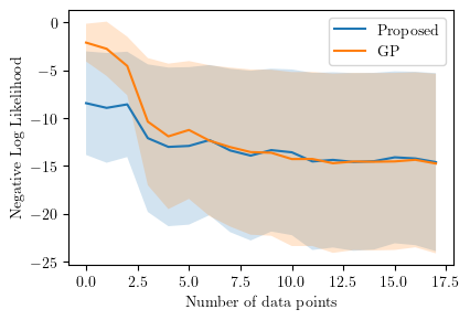
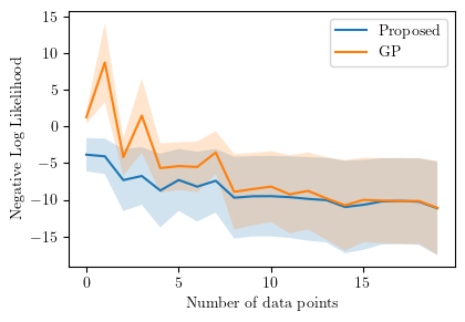
We first show the negative log-likelihood (NLL) of the predictions for the cases (I) and (II) discussed in Section VI, in Figure 6. The NLLs against the number of data points are calculated for both the proposed scheme and the case where we use Gaussian process regression (GPR) instead of ALPaCA. NLLs are calculated for 100 different obstacles and the average and 3- intervals are plotted in the figures. Note that the number of data points in the figures means the number of surface points and the actual number of data points is () times of that. The squared exponential kernel is used for GP and the parameters in the kernel are fitted by solving the maximum likelihood problem. In GP implementation, the Python library GPy [45] is used. From the figures, we can see that the prediction made by the proposed meta-learning scheme is superior to that of the GPR case when the number of data is small. The time analysis is also provided in Figure 7. Figure 7 shows that the proposed scheme can produce the prediction very fast compared to the case in which every time fits the GP, which is especially beneficial for the usage of the online synthesis of CBF-QP since we can more frequently update the CBFs. Additional examples of the prediction are shown in Figure 8a and 8b.
-D Detailed Results for Control Execution
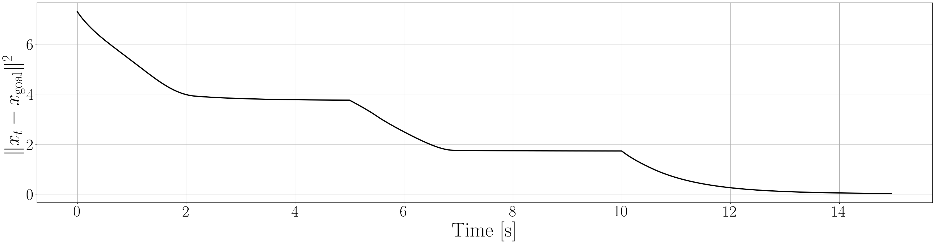
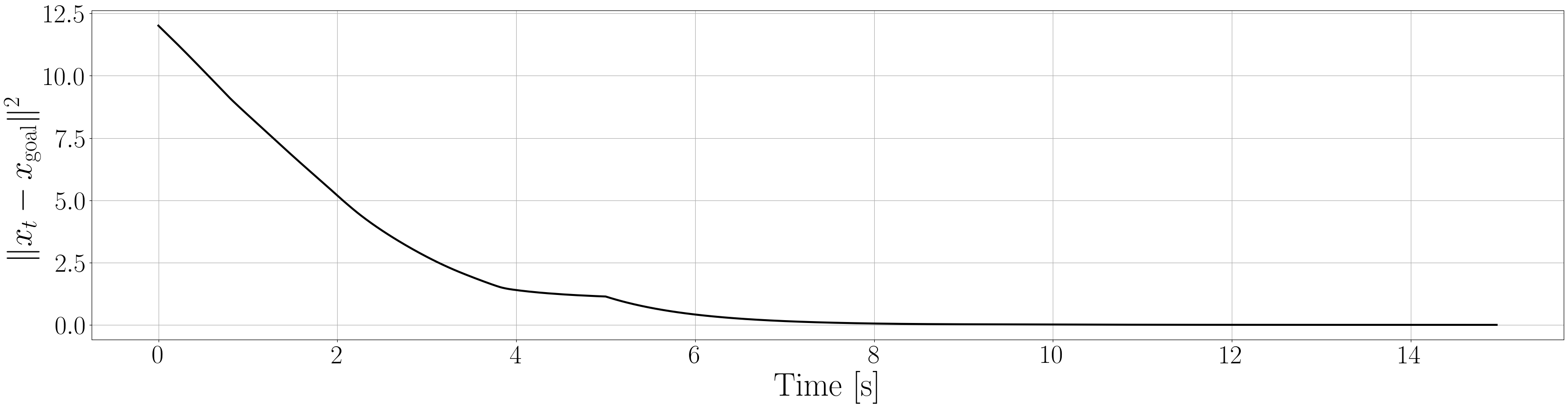
Next, we summarize the detailed results for control execution. In Figures 8– 12, we show the resulting trajectories and the time evolution of the squared errors between the robot positions and the goal positions when , for all 6 environments. From these figures, we can see that the tight prediction of the proposed scheme leads to less conservative control performance as explained in Section VI. In Table LABEL:CSE, we also summarize the cumulative squared errors between the robot position and goal position for all environments and the cases [s].

| Proposed | GP | |||||
|---|---|---|---|---|---|---|
| Environment / | 1 | 3 | 5 | 1 | 3 | 5 |
| 1 | 554.93 | 620.12 | 618.56 | 543.78 | 715.75 | 1010.93 |
| 2 | 654.10 | 702.75 | 830.22 | 697.65 | 818.47 | 1094.79 |
| 3 | 534.40 | 585.63 | 654.25 | 533.77 | 609.42 | 897.31 |
| 4 | 794.06 | 794.06 | 843.25 | 1792.50 | 1792.50 | 1803.99 |
| 5 | 475.41 | 475.41 | 486.61 | 472.43 | 472.43 | 503.12 |
| 6 | 1068.52 | 1068.56 | 1076.81 | 1271.35 | 1271.32 | 1648.49 |