Bayesian inference via geometric optics approximation

Zejun Sun School of Mathematics, Hunan University, Changsha 410082, China. Email: [email protected] Guang-Hui Zheng School of Mathematics, Hunan Provincial Key Laboratory of Intelligent Information Processing and Applied Mathematics, Hunan University, Changsha 410082, China. Email: [email protected] (Corresponding author)

ABSTRACT

Markov chain Monte Carlo (MCMC) simulations have been widely used to generate samples from the complex posterior distribution in Bayesian inferences. However, these simulations often require multiple computations of the forward model in the likelihood function for each drawn sample. This computational burden renders MCMC sampling impractical when the forward model is computationally expensive, such as in the case of partial differential equation models. In this paper, we propose a novel sampling approach called the geometric optics approximation method (GOAM) for Bayesian inverse problems, which entirely circumvents the need for MCMC simulations. Our method is rooted in the problem of reflector shape design, which focuses on constructing a reflecting surface that redirects rays from a source, with a predetermined density, towards a target domain while achieving a desired density distribution. The key idea is to consider the unnormalized Bayesian posterior as the density on the target domain within the optical system and define a geometric optics approximation measure with respect to posterior by a reflecting surface. Consequently, once such a reflecting surface is obtained, we can utilize it to draw an arbitrary number of independent and uncorrelated samples from the posterior measure for Bayesian inverse problems. In theory, we have shown that the geometric optics approximation measure is well-posed. The efficiency and robustness of our proposed sampler, employing the geometric optics approximation method, are demonstrated through several numerical examples provided in this paper.

keywords: Bayesian inference, geometric optics approximation, sampling method, reflector shape design

1 Introduction

In recent years, Bayesian inference has gained considerable popularity for modeling and solving inverse problems across a wide range of scientific and engineering disciplines [18, 12]. The process of inferring unknown parameters from noisy measurement data is prevalent in various applications, including physical processes, biological models, and engineering systems. Bayesian inference offers a valuable framework for addressing these challenges, as it allows for the quantification of uncertainties in the obtained solution by leveraging statistical information such as moments and confidence intervals. A typical Bayesian approach to inverse problems involves updating the knowledge of unknown parameters from a prior distribution to a posterior distribution. This update is accomplished by incorporating the likelihood function, which describes the data given the parameters. The likelihood function can be determined by combining an assumed error distribution with a forward model that maps parameters to observations. By integrating these components within the Bayesian framework, a comprehensive analysis of the inverse problem can be conducted, enabling the characterization of uncertainties and providing a more holistic understanding of the underlying system.

Let $\mu_{0}$ be a prior probability measure on $\mathbb{R}^{n}$ and $\Phi_{y}:\mathbb{R}^{n}\to[0,+\infty)$ denotes a measurable negative log-likelihood function. Bayes theorem then yields the posterior probability measure

\displaystyle\mu^{y}(\,\mathrm{d}x)=\frac{1}{Z}\exp(-\Phi_{y}(x))\mu_{0}(\,\mathrm{d}x),\quad Z:=\int_{\mathbb{R}^{n}}\exp(-\Phi_{y}(x))\mu_{0}(\,\mathrm{d}x).

(1.1)

In this context, the posterior measure plays a crucial role in characterizing both the parameter values and their associated uncertainties. However, when tackling a Bayesian inverse problem, it becomes essential to explore and analyze the posterior measure through techniques such as sampling or integration. One widely used and flexible approach for drawing samples from the complex posterior probability distribution in Bayesian inference is Markov chain Monte Carlo (MCMC) simulations [12, 28, 32]. Nevertheless, when utilizing MCMC simulations, a notable challenge arises: the forward model within the likelihood function often needs to be evaluated multiple times for each sample drawn at different parameter values. Consequently, if the computation of each forward model, such as in the case of partial differential equation models, is computationally expensive, the practical feasibility of MCMC sampling diminishes rapidly.

This paper introduces a novel sampling method, the geometric optics approximation method (GOAM), which offers a direct means of drawing samples from the posterior measure for Bayesian inverse problems, completely circumventing the need for MCMC simulations. Our approach is based on the problem of reflector shape design, which encompasses the design of reflector antennas, beam-shaping systems, mirrors, and related areas. Reflectors have been extensively studied by researchers, particularly in the fields of electromagnetism and optics [10, 11]. The fundamental problem in reflector design involves determining a reflecting surface within an optical system that can transform a given light distribution across a source domain into a desired light distribution across a target domain. This problem has garnered significant attention and has been the subject of extensive investigation by researchers. By leveraging the principles and techniques from this field, we propose the GOAM sampler as a means to draw samples from the posterior measure.

Figure 1.1: The reflector optical system

We consider the reflector system consisting of a reflecting hypersurface $R$ , a point source of light placed at origin $\mathcal{O}$ of a Cartesian coordinate system in space $\mathbb{R}^{n+1},\;n\geq 2$ , and a bounded smooth target domain $\Omega$ in a hyperplane $P:=\{x_{n+1}=h|h\leq 0\}$ to be illuminated. Assume that the source $\mathcal{O}$ , a reflecting hypersurface $R$ , and a target $\Omega$ are positioned so that the rays emitted by the source through an input aperture $\varGamma$ in the unit sphere, i.e., $\varGamma\subset S^{n}$ , and $\Omega_{\Gamma}$ is the projection of $\Gamma$ onto a horizontal plane $x_{1}Ox_{2}$ , where $S^{n}$ is the unit sphere centred at origin in $\mathbb{R}^{n+1}$ , fall on the reflecting surface $R$ and are incident on the target domain $\Omega$ . Let $I\in L^{1}(\varGamma)$ be the intensity of light from the source, and let $L\in L^{1}(\Omega)$ be a nonnegative function on $\Omega$ . The reflector shape design problem is concerned with constructing of reflector surface $R$ such that rays from a source with the density $I$ is reflected off to the target domain $\Omega$ which creates a prescribed in advance density $L$ ; see Fig.1.1 for the reflector optical system in $\mathbb{R}^{3}$ . A special case of the reflector shape design problem is the so-call far field reflector design case, or the reflector antenna design, which can be regarded as the limit of the above problem with $h\to-\infty$ . Namely, the target domain is assumed to be infinitely far away from the light source. In this article, we only consider the near-field case, and in the far-field case all results can be restated without any essential changes. The reflecting surface $R$ is represented by a vector function

\displaystyle R(m)

\displaystyle=m\rho(m),\quad m\in\varGamma,

(1.2)

where $\rho$ is the polar radius and a smooth positive function defined in $\varGamma$ . Let $\upsilon$ denote the unit normal vector of $R$ . Then from the law of reflection, the reflection direction is

\displaystyle y

\displaystyle=m-2(m\cdot\upsilon)\upsilon,

(1.3)

where $m\cdot\upsilon$ denotes the inner product in $\mathbb{R}^{n+1}$ . Hence

\displaystyle z=T(m)=m\rho(m)+y(m)d(m),\quad m\in\varGamma,

(1.4)

where $d(m)$ is the distance from reflecting surface $R$ to the target domain $\Omega$ in the direction $y$ and $T:\varGamma\rightarrow\Omega$ is the reflection mapping.

A natural idea, therefore, is to construct a reflecting surface within a reflector optical system that can transport a given simple distribution over a source domain to the posterior measure on the target domain. In this context, the objective is for the light originating from the source to be reflected onto the target domain in such a way that the distribution of reflected light accurately aligns with the posterior measure. In essence, the Bayesian posterior measure can be regarded as a reflection mapping of the source distribution. Once this reflecting surface (i.e., reflection mapping $T$ ), is determined, the reflector system can be utilized to generate an arbitrary number of independent and uncorrelated samples from the posterior distribution. More simply, imagine generating rays from origin with vectors $m_{i}\in\varGamma$ according to the source distribution, and then reflecting each ray off at a point $R(m_{i})$ in direction $y(m_{i})$ , and reaching a point $z=T(m_{i})$ that is distributed according to the posterior. To ascertain the desired reflecting surface or reflection mapping, it is imperative to tackle the reflector shape design problem. This problem encompasses the task of finding the optimal configuration for the reflecting surface within the reflector system. Its solution holds the key to achieving the desired transformation of the light distribution from the source domain to the target domain.

The design of freeform optical reflector surfaces, without prior assumptions regarding symmetries, can be approached by formulating a partial differential equation. This equation is derived from the principles of geometric optics and energy conservation, capturing the geometric deformation of energy density by the reflecting surface. By incorporating the law of reflection, a reflection mapping connecting coordinates on the aperture $\varGamma$ and domain $\Omega$ can be constructed. Substituting this mapping into the energy conservation relation leads to a fully nonlinear second-order elliptic partial differential equation, known as a generalized Monge-Ampère equation. This equation possesses an unusual boundary condition referred to as the transport boundary condition [29, 24, 36, 17, 19]. The existence and uniqueness of weak solutions for reflector design problems have been established through the approximation of piecewise ellipsoid surfaces [20, 2, 19]. The local interior regularity of reflector problems has also been investigated in [19]. A provably convergent numerical algorithm called the supporting ellipsoid method has been introduced, explicitly determining the ellipsoid required to construct the reflectors [20, 21]. Variations of this method, including the exploration of supporting ellipsoids, have been extensively studied in [9, 4]. The far-field case has been considered in references [36, 2], and a variant utilizing paraboloids of revolution in place of ellipsoids was developed in [3]. In [1], the solution to reflector design problems was obtained by numerically solving the Monge-Ampère type equation using a collocation method based on tensor-product B-splines.

The second-order elliptic partial differential equations of the Monge-Ampère type frequently arise in the realm of optimal transport problems. In these problems, the objective is to identify a transport plan that minimizes a cost function associated with the transportation process. This cost function is typically an integral of a cost function weighted by the reference distribution, ensuring the preservation of total mass [35, 34]. By applying duality, the reflector antenna system, which aims to transform the energy distribution of a point source into a desired far-field distribution, can be formulated as an optimal transport problem. In this formulation, a logarithmic cost function is employed [37]. The optimal transport problem associated with the far-field case can be cast as a linear optimization problem, allowing for its solution using linear programming techniques [37]. On the other hand, the near-field reflector shape design problem is not an optimal transport problem [19, 15]. The near-field reflector system gives rise to a transportation problem with a cost function that depends non-linearly on a potential and it has been shown that the weak solution of the near-field reflector problem do not optimize this cost functional [15].

In the context of Bayesian inverse problems, [23, 7] have presented an approach that explicitly construct a transport map that pushes forward the prior measure to the posterior measure. This transport map is found through the solution of a variational problem. In this paper, our sampling method is based on the reflector shape design, where the reflection mapping $T$ in (1.4) or the reflecting surface can also be viewed as a ‘transport map’ connecting the source distribution and the target distribution. However, we emphasize that the design of the reflector shape problem, upon which this sampling method is based, is distinct from an optimal transport problem. [19, 15], which is different from the literature [23, 7]. The key idea is to define the target distribution on target domain in optical systems as the unnormalized posterior distribution for Bayesian inference. Consequently, a geometric optics approximation measure can be defined by the reflector for the posterior. We have proved stability of this measure with respect to the target domain. The existence and uniqueness of the weak solution for the reflector shape design problem have been proved in [20, 2, 19]. To solve the reflector shape design problem, we use the method of supporting ellipsoids [21]. Once the desired reflecting surface is obtained, the reflection mapping or reflector can be utilized to draw an arbitrary number of effective samples from the posterior measure, and we thereby entirely avoid MCMC simulations. We substantiate the performance of our proposed sampling method through a series of numerical experiments, demonstrating its efficiency and robustness when using geometric optics approximation. In summary, the main contributions in this article are the following:

•

We introduce a novel sampling method that leverages the geometric optics approximation for Bayesian inference. The proposed method reveals the inherent connection between Bayesian inverse problems and the reflector shape design problem, and thus offers a valuable approach to address the challenges associated with sampling in Bayesian inference.
•

We provide a rigorous mathematical analysis for the geometric optics approximation measure established by the reflector design for the Bayesian posterior. In particular, we prove the stability of the geometric optical approximation posterior measure, which ensures the numerical stability of sampling the posterior measure.
•

The proposed direct sampler utilizing the geometric optics approximation which based on supporting ellipsoid method, can cheaply generate an arbitrary number of independent and unweighted samples from posterior distribution. However, unlike the optimal transport method [7], it obviates the necessity of solving high-dimensional optimization problems. Thus, our method exhibits notable efficiency and robustness, entirely avoids the need for computationally intensive MCMC simulation.
•

In comparison to MCMC method, our proposed approach demonstrates notable enhancement in computational efficiency, particularly in the challenging task of solving multi-parameter inversion problems for nonlinear models. Meanwhile, the extensive applicability of our method is demonstrated through various numerical examples of different types, which contains locating acoustic source problem, determining fractional orders for time-space fractional diffusion equation, and simultaneous reconstruction of multi-parameters in nonlinear advection-diffusion-reaction model.

The subsequent sections of this paper are structured as follows: Section 2 presents a comprehensive description of the Bayesian inverse problem framework, outlining its fundamental principles and methodologies. In Section 3, the mathematical formulation of reflector shape design is introduced, providing a detailed explanation of the underlying mathematical concepts and techniques. The application of the geometric optics approximation for Bayesian inference is elucidated in Section 4, highlighting its relevance and implications within the context of the problem under investigation. Section 5 focuses on describing the sampling procedure utilizing the geometric optics approximation, presenting a step-by-step account of the methodology employed. In order to showcase the efficacy and robustness of the geometric optics approximation method, Section 6 presents a series of numerical examples, offering empirical evidence and analysis.

2 The Bayesian framework

Let $\mathbf{X}$ be a separable Hilbert space, equipped with the Borel $\sigma$ -algebra, and $\mathcal{G}:\mathbf{X}\to\mathbb{R}^{n}$ be a measurable function called the forward operator, which represents the connection between parameter and data in the mathematical model. We wish to solve the inverse problems of finding the unknow model parameters $u$ in set $\mathbf{X}$ from measurement data $y\in\mathbb{R}^{n}$ , which is usually generated by

\displaystyle y=\mathcal{G}(u)+\eta,

(2.1)

where the noise $\eta$ is assumed to be a $n$ -dimensional zero-mean Gaussian random variable with covariance matrix $\Sigma_{\eta}$ . In Bayesian inverse problems, the unknown model input and the measurement data are usually regarded as random variables. From (2.1), we define the negative log-likelihood

\Phi_{y}(u):=\frac{1}{2}\|\Sigma_{\eta}^{-\frac{1}{2}}(\mathcal{G}(u)-y)\|^{2}_{2},

with the Euclidean norm $\|\cdot\|_{2}$ . Combining the prior probability measure $\mu_{0}$ with density $\pi_{0}$ and (1.1) gives the posterior density up to a normalizing constant

\displaystyle\pi(u)=\exp\bigl{(}-\Phi_{y}(u)\bigr{)}\pi_{0}(u).

(2.2)

3 Mathematical formulation of reflector shape design

In this section, we derive the partial differential equation which describes the shape of the reflector that transforms lights from a point source into a specified output intensity distribution in the near field.

In this paper, we always assume that there is no loss of energy in the reflector system. Then we have the energy conservation:

\displaystyle\int_{E}I(m)d\sigma(m)=\int_{T(E)}L(z)\,\mathrm{d}\mu(z)

(3.1)

for any open set $E\subset\varGamma$ , where $\sigma$ is a standard measure on $S^{n}$ and $\mu$ is the Lebesgue measure on $\Omega$ . Note that

\int_{T(E)}L(z)d\mu(z)=\int_{E}L\bigl{(}T(m)\bigr{)}\bigl{|}\det\bigl{(}J(T)\bigr{)}\bigr{|}\,\mathrm{d}\sigma(m),

where $\det\bigl{(}J(T)\bigr{)}$ is the Jacobian determinant of the map $T$ . Therefore, we obtain

\displaystyle\bigl{|}\det\bigl{(}J(T(m))\bigr{)}\bigr{|}=\frac{I(m)}{L\bigl{(}T(m)\bigr{)}},\quad m\in\varGamma.

(3.2)

The corresponding boundary condition is the natural one

\displaystyle T(\varGamma)=\Omega.

(3.3)

A necessary compatibility condition for the reflector problem is the energy conservation

\displaystyle\int_{\varGamma}I(m)d\sigma(m)=\int_{\Omega}L(z)\,\mathrm{d}\mu(z).

(3.4)

Let $(t^{1},t^{2},\dots,t^{n})$ be a smooth parametrization of $S^{n}$ . Then $m=m(t^{1},t^{2},\dots,t^{n})$ . Denote by $(e_{ij})=(\partial_{i}m\cdot\partial_{j}m)$ the matrix of coefficients of the first fundamental forms of $S^{n}$ , where $\partial_{i}=\partial/\partial t^{i}$ . Put $(e^{ij})=(e_{ij})^{-1}$ and $\nabla=e^{ij}\partial_{j}m\partial_{i}$ . Then the unit normal vector of $R(m)=m\rho(m)$ is given by

\displaystyle\upsilon=\frac{\nabla\rho-m\rho}{\sqrt{\rho^{2}+|\nabla\rho|^{2}}},

(3.5)

where $|\nabla\rho|^{2}=e^{ij}\partial_{j}\rho\partial_{i}\rho$ . Indeed, the unit normal vector (3.5) can be obtain by $\partial_{1}R\times\partial_{2}R\times\dots\times\partial_{n}R$ where $\times$ denotes the outer product in space $\mathbb{R}^{n+1}$ .

For simplicity in computing the Jacobian determinant of $T$ , we choose an orthonormal coordinate system on $S^{n}$ near the north pole. Assuming that $\varGamma$ is in the north hemisphere, i.e., $\varGamma\subset S^{n}_{+}$ where $S^{n}_{+}:=S^{n}\cap\{x_{n+1}>0\}$ , let $m=(m_{1},m_{2},\cdots,m_{n+1})\in\varGamma$ satisfying

\displaystyle\begin{cases}m_{k}(t^{1},t^{2},\dots,t^{n})&=t^{k},\quad k=1,2,\dots,n\\ m_{n+1}(t^{1},t^{2},\dots,t^{n})&=w,\end{cases}

(3.6)

and $\|t\|_{2}<1$ , where $w:=\sqrt{1-\|t\|_{2}^{2}}$ and $t=(t^{1},t^{2},\dots,t^{n})\in\Omega_{\varGamma}\subset\mathbb{R}^{n}$ . Therefore we may also regard $\rho=\rho(t)$ as a function on $\Omega_{\varGamma}$ and $T=T(t)$ as a mapping on $\Omega_{\varGamma}$ .

Theorem 3.1.

Let $\varGamma\subset S^{n}_{+}$ and $\Omega\subset P$ , and let the density functions $I\in L^{1}(\varGamma)$ and $L\in L^{1}(\Omega)$ be given, satisfying the energy conservation (3.1). For the polar radius $\rho$ of reflecting surface $R$ in the reflector shape design problem, define $u:=1/\rho$ , and

a:=\|Du\|^{2}_{2}-(u-Du\cdot t)^{2},\quad b:=\|Du\|^{2}_{2}+u^{2}-(Du\cdot t)^{2},

where $Du=(\partial_{1}u,\partial_{2}u,\dots,\partial_{n}u)$ is the gradient of $u$ , and

\mathcal{M}:=1+\frac{t\otimes t}{1-\|t\|_{2}^{2}},\quad c:=\frac{h}{w},

where $t\otimes t=(t^{i}t^{j})$ is an $n\times n$ matrix. Then the $u$ is governed by the equation

\displaystyle\det\biggl{(}D^{2}u+\frac{ca}{2(1-cu)}\mathcal{M}\biggr{)}=\frac{|a^{n+1}|}{2^{n}(1-cu)^{n}b}\cdot\frac{I(t)}{wL\circ T(t)},\quad t\in\Omega_{\varGamma},

(3.7)

where $D^{2}u=(\partial_{i}\partial_{j}u)$ is the Hessian matrix of $u$ .

The second order elliptic partial differential equation governing the near field reflector problem is a fully nonlinear equation of Monge-Ampère type whose proof is similar to [19]. But, for the self-containedness, we still give the proof in Appendix A.

Remark 3.1.

Substituting $u=1/\rho$ into equation (3.7), we can obtain the equation

\displaystyle\det\biggl{(}-D^{2}\rho+\frac{2}{\rho}D\rho\otimes D\rho+\frac{c\tilde{a}}{2\rho(\rho-c)}\mathcal{M}\biggr{)}=\frac{|\tilde{a}^{n+1}|}{2^{n}\rho^{n}(\rho-c)^{n}\tilde{b}}\cdot\frac{I(t)}{wL\circ T(t)}

(3.8)

for $\rho$ , where $\tilde{a}=\|D\rho\|^{2}_{2}-(\rho+D\rho\cdot t)^{2}$ and $\tilde{b}=\|D\rho\|^{2}_{2}+\rho^{2}-(D\rho\cdot t)^{2}$ .

ii)

Here if $\rho=1/u$ is a convex solution (see [19]), the matrix $\{D^{2}u+\frac{ca}{2(1-cu)}\mathcal{M}\}$ is positive definite. Noting that $\varGamma\subset S^{n}_{+}$ , we have $m_{n+1}>0$ and $y_{n+1}<0$ . Hence by (A.4),

$a=\frac{y_{n+1}}{m_{n+1}}b<0.$

Therefore when $n$ is odd, the right-hand side of (3.7) should take absolute value.
iii)

If one set $\Omega\subset\{x_{n+1}=0\}$ , i.e., $h=0$ , then the (3.7) simplifies to

$\displaystyle\det(D^{2}u)=\frac{|a^{n+1}|}{2^{n}b}\cdot\frac{I(t)}{wL\circ T(t)},$ (3.9)

which is a standard Monge-Ampère equation.

4 Geometric optics approximation for Bayesian inference

The reflector shape design problem is to recover the reflector surface $R$ such that rays from a source is reflected off to the target domain $\Omega$ and the density of reflected light on $\Omega$ is equal to a prescribed in advance density $L$ . For Bayesian inference, in this work, $L$ takes the value of the unnormalized posterior density (2.2) on domain $\Omega$ , i.e.,

\displaystyle L(x):=\pi(x),\quad x\in\Omega,

(4.1)

which can be regarded as a unnormalized posterior density on $\Omega$ . Here we do not need a normalized posterior density, but only the energy conservation. In the reflector system, if a reflecting surface $R$ is determined such that the energy from source with density $I$ , redirected by $R$ , is distributed on target $\Omega$ producing the intensity $L$ , the reflecting mapping $T$ can be obtained by (1.4) and it transforms a random variable $X$ , distributed according to the source distribution, into the another random variable $Z=T(X)$ , distributed according to the posterior.

An approach in [23, 7] is presented for Bayesian inference that explicitly construct a transport map that pushes forward the reference measure to the target measure, and the transport map is actually found through the solution of variational problem, namely

\displaystyle\min_{T\in\mathcal{T}}\mathcal{D}_{KL}(I\|T^{\sharp}L),

(4.2)

where $\mathcal{D}_{KL}(\cdot\|\cdot)$ is the Kullback-Leibler divergence, $T^{\sharp}L:=L\circ T|\det(J(T))|$ is the pullback of density $L$ , and $\mathcal{T}$ is some space of lower-triangular function. Any global minimizer of (4.2) achieves the minimum $\mathcal{D}_{KL}(I\|T^{\sharp}L)=0$ and implies that $I=T^{\sharp}L$ . In fact, finding such a global minimizer, i.e., the transport map $T$ , is very difficult, especially when the target measure contains a partial differential equation model. In this paper, the reflection mapping $T$ in (1.4) can also be viewed as a ‘transport map’. In our context, it does not necessitate solving an optimization problem to obtain the transport map. Instead, it can be formulated as the problem of determining the shape of the reflector, which is described by the Monge-Ampère type equation (3.8).

4.1 Geometric optics approximation measure

In the study of the reflector problem, ellipsoid of revolution plays a crucial role (in the far field case it is paraboloid of revolution). A ray from one focus will always be reflected to the other one in an ellipsoid. Let $z\in\mathbb{R}^{n+1},\,z\neq\mathcal{O}$ . Denote by $E_{z}(d)$ an ellipsoid of revolution with major axis $\mathcal{O}z$ , foci $\mathcal{O}$ and $z$ , and the focal parameter $d$ . In this paper, the ellipsoid refers to this kind of ellipsoid where one of the foci is always placed at $\mathcal{O}$ . Any such ellipsoid is uniquely defined by $\mathcal{O},z,d$ and can be represented

E_{z}(d)=\{x\rho_{z}(x)|x\in S^{n}\}

with

\displaystyle\rho_{z}(x)=\frac{d}{1-\varepsilon(\hat{z}\cdot x)},

(4.3)

where $\hat{z}=z/\|z\|_{2}$ and

\varepsilon=\sqrt{1+\frac{d^{2}}{z^{2}}}-\frac{d}{|z|}

is the eccentricity.

Definition 4.1.

Let $R=R_{\rho}$ be a reflecting surface, given by (1.2). An ellipsoid $E_{z}(d),z\in\Omega,d\geq 0$ , is called supporting to $R_{\rho}$ at $m\in\varGamma$ if $\rho(m)=\rho_{z}(m)$ and $\rho(x)\leq\rho_{z}(x),\forall x\in\varGamma$ .

Definition 4.2.

The reflecting surface $R=R_{\rho}$ is called convex with respect to $\Omega$ if for any $m\in\varGamma$ , there is a supporting ellipsoid at $m$ . Moreover, if $R$ is also a piecewise ellipsoidal surface, namely

\displaystyle R=\bigcup^{K}_{i=1}(E_{z_{i}}\cap R),

(4.4)

where $z_{i}\in\Omega$ , we say reflecting surface $R$ is an polyhedron with respect to $\Omega$ .

Remark 4.1.

Similarly, we have the concave reflecting surface. We say a reflecting surface $R=R_{\rho}$ is concave if for any point $m\in\varGamma$ , there is an ellipsoid $E_{z}(d)$ , with the foci $z$ on $\Omega$ , which satisfies $\rho(m)=\rho_{z}(m)$ and $\rho(x)\geq\rho_{z}(x),\forall x\in\varGamma$ .

Remark 4.2.

A solution to reflector shape design is convex if it fulfills ellipticity constraint, i.e. the matrix $D^{2}u+\frac{ca}{2(1-cu)}\mathcal{M}$ in (3.7) is positive definite. Moreover, a solution is concave so that this matrix is negative definite.

Remark 4.3.

For a reflector, we can approximate it by an polyhedron. If the reflecting surface is an polyhedron, there are two possible geometries, i.e. convex or concave. The body bounded by $E_{z_{i}}$ we denote by $B_{z_{i}}$ . We say that an polyhedron $R$ is convex, or concave, if it is given by

\displaystyle R=\partial B\quad\text{where}\;B=\bigcap^{K}_{i=1}B_{z_{i}},

(4.5)

\displaystyle R=\partial B\quad\text{where}\;B=\bigcup^{K}_{i=1}B_{z_{i}},

(4.6)

respectively, for a finite number of ellipsoids $E_{z_{1}},E_{z_{2}},\dots,E_{z_{K}}$ and $\partial B$ is the boundary of $B$ . We can obtain convex reflector geometries if the set of ellipsoid facets closest to the source are used. Conversely, concave reflector geometries are obtained if the set of ellipsoid facets away from the source are used. The choice of desired geometry sets the rule that determines which rays are reflected by which ellipsoid. The difference between the two geometries is whether the rays cross each other after reflection.

For a convex reflector $R_{\rho}$ , we have

\displaystyle\rho(x)=\inf_{z\in\Omega}\frac{d(z)}{1-\varepsilon(d(z))(\hat{z}\cdot x)},\quad x\in\varGamma.

(4.7)

Since for each $z\in\Omega$ the ellipsoid $E_{z}(d(z))$ is supporting to $R_{\rho}$ , we also have

\displaystyle d(z)=\sup_{x\in\varGamma}\rho(x)(1-\varepsilon(d(z)))(\hat{z}\cdot x),\quad z\in\Omega.

(4.8)

Note that the $\inf$ in (4.7) and $\sup$ in (4.8) are achieved at some $z\in\Omega$ and $x\in D$ , respectively.

For the reflecting surface $R_{\rho}$ , we define two maps (possible multiple valued)

T(x)=\{z\in\Omega|d(z)=\rho(x)(1-\varepsilon(d(z)))(\hat{z}\cdot x)\},\quad x\in\varGamma,

and

V(z)=\{x\in\varGamma|d(z)=\rho(x)(1-\varepsilon(d(z)))(\hat{z}\cdot x)\},\quad z\in\Omega.

That is, $T$ maps direction $x\in\varGamma$ to the foci $z\in\Omega$ of an ellipsoid supporting to $R_{\rho}$ at $R(x)$ . And $V$ represents that there exists an supporting ellipsoid of $R_{\rho}$ at $R(x)$ with $z$ as its foci. Note that $T$ is single valued and is exactly the reflection mapping at any differentiable point of $\rho$ . If the $R_{\rho}$ is the smooth surface and the map $T$ is a diffeomorphism, then $V=T^{-1}$ . We denote

\displaystyle V(\omega)

\displaystyle=\bigcup_{z\in\omega}V(z),\quad\omega\subseteq\Omega,

(4.9)

and

\displaystyle T(\omega)

\displaystyle=\bigcup_{x\in\omega}T(x),\quad\omega\subseteq\varGamma.

(4.10)

Because the image of $w$ in the target $\Omega$ is the set of all directions $x\in\varGamma$ in which the set $\omega$ is visible for the source, the set $V(\omega)$ is called the visibility set of $\omega$ [20].

Let a reflecting surface $R$ be an polyhedron, as given in (4.4). We choose points $z_{1},z_{2},\dots,$ $z_{K}\in\Omega$ as the foci of the ellipsoids $E_{z_{1}},E_{z_{2}},\dots,E_{z_{K}}$ . Then $V(z_{i})=R\cap E_{z_{i}}$ for any $i\in\{1,2,\dots,K\}$ and the set $V(\Omega^{\prime})$ has measure zero, where $\Omega^{\prime}=\Omega\setminus\{z_{1},z_{2},\dots,z_{K}\}$ . By this approximation, if $R$ is the convex surface, for any Borel set $w\subset\Omega$ , then $V(w)$ is Borel. Hence we define a Borel measure on $\Omega$ by

\displaystyle\mu_{R}(\omega):=\int_{V(\omega)}I(x)\,\mathrm{d}\sigma(x),\quad\forall\omega\subseteq\Omega.

(4.11)

The $\mu_{R}(\omega)$ represents the total energy ‘delivered’ by reflector $R$ from $\mathcal{O}$ through $V(\omega)$ to set $\omega$ and it is a non-negative and countable additive measure on the Borel set of $\Omega$ . If we set, for any Borel set $U$ of $\varGamma$ ,

\displaystyle\mu_{s}(U)=\int_{U}I(x)\,\mathrm{d}\sigma(x),

(4.12)

which is the measure of source on the $\varGamma$ , then $\mu_{R}$ is the push-forward of $\mu_{s}$ with map $T$ , namely

\mu_{R}(\omega)=\mu_{s}(V(\omega)).

We put

\displaystyle\mu_{t}(U)=\int_{U}L(x)\,\mathrm{d}\mu(x),

(4.13)

for any Borel set $U$ of $\Omega$ .

Definition 4.3.

A reflecting surface $R$ is called the weak solution to the reflector shape design problem if it satisfies

\displaystyle\mu_{R}(\omega)=\mu_{t}(\omega),

(4.14)

for any Borel set $\omega\subset\Omega$ . Furthermore, if the density $L$ in $\mu_{t}$ satisfies (4.1) on $\Omega$ , we say that the measure $\mu_{R}$ is the geometric optics approximation measure with respect to the unnormalized posterior $\mu^{y}$ on the target domain $\Omega$ .

In the next subsection, we will study the well-posedness of the push-forward of $\mu_{s}$ , i.e., existence, uniqueness and stability of the geometric optics approximation measure $\mu_{R}$ .

4.2 Well-posedness

To investigate the well-posedness of the geometric optics approximation measure $\mu_{R}$ , we first examine the existence, uniqueness, and stability of weak solutions to the reflector shape design problem. The study of weak solutions has been addressed in previous works, such as [20] and [19]. In [20], the authors established the existence and uniqueness of weak solutions. An extension of the existence of weak solutions and their regularity can be found in [19].

A basic property of $\mu_{R}$ is its weak continuity [20], which is necessary for proving the existence of the solution to reflector shape design problem and the well-posedness of geometric optics approximation measure $\mu_{R}$ .

Lemma 4.1.

Let $R^{K},K=1,2,\dots$ be a sequence of convex reflectors which converges to a convex reflector $R$ locally uniformly, then the measure $\mu_{R^{K}}$ converges weakly to the measure $\mu_{R}$ .

A proof of Lemma 4.1 can be found in [20]. The weak continuity is valid for general convex reflectors, not necessarily defined by a finite number of ellipsoids.

Theorem 4.2 (Existence and uniqueness of weak solution).

Let $\Omega$ be a bounded smooth domain in $P$ and $\varGamma\subset S^{n}$ . Consider the reflector shape design problem with $I\in L_{1}(\varGamma),I\geq 0$ and $L\in L_{1}(\Omega),L\geq 0$ satisfying the energy conservation (3.4). Then for any point $p$ be on the light cone $\mathcal{C}_{\varGamma}$ of the source, i.e.

p\in\mathcal{C}_{\varGamma}:=\biggl{\{}p\in\mathbb{R}^{n+1}\bigg{|}\frac{p}{\|p\|_{2}}\in\varGamma\biggr{\}},

and satisfying $\|p\|_{2}>2\sup_{z\in\Omega}\|z\|_{2}$ , there exists a weak solution, namely the reflecting surface $R$ satisfying the equation (4.14), to the reflector problem such that $R$ passes through the point $p$ . And the weak solution $R$ is unique up to the choosing of the point $p\in\mathcal{C}_{\varGamma}$ and searching for convex or concave reflecting surface.

The proof of this theorem is given in [20, 19] based on geometric ideas by approximation by convex polyhedra. In brief, the key steps of the proof are as follows. First, the measure $\mu_{t}$ is approximated by a sequence $\mu_{t}^{K},K=1,2,\dots,$ of finite sums of Dirac measure concentrated at some point $z_{1},z_{2},\dots,z_{K}\in\Omega$ . For a fixed point $p$ and each $\mu_{t}^{K}$ , a solution $R^{K}$ of (4.14) with the right-hand side replaced by $\mu_{t}^{K}$ is determined by an polyhedron, i.e., envelope of a finite number of ellipsoids with one foci at $\mathcal{O}$ and the other foci at $z_{i},i=1,2,\dots,K$ , which passes through the point $p$ . One can prove that such solution can always be found by a special monotonically convergent process. Then let $K\rightarrow\infty$ and use the weak continuity of the measure $\mu_{t}^{K}$ and $\mu_{R^{K}}$ , $R^{K}$ converges to a weak solution $R$ , which passes through the point $p$ .

Furthermore, the existence proof is constructive and it can be transformed into a convergent numerical procedure [21]. In section 5.1, we describe the method of supporting ellipsoid to solve the reflector shape design problem.

Remark 4.4.

Note that the solution is not unique, if there is a solution for a point $p\in\mathcal{C}_{\varGamma}$ , we know that there exist other solution containing the point $cp$ for $c>1$ . Even if we fix point $p\in\mathcal{C}_{\varGamma}$ , there still exist at least two solutions passing through point $p$ , i.e., the convex and concave solution. In [19], one can find a proof that there are a convex and concave solution for any fixed point $p\in\mathcal{C}_{\varGamma}$ . Therefore, the weak solution $R$ is unique up to the choosing of one point $p\in\mathcal{C}_{\varGamma}$ , i.e., the size of the reflector, and searching for convex or concave solution, which is a necessary condition to ensure well-posedness of the reflector shape design problem.

Remark 4.5.

The regularity of the solution strongly depends on the regularity of the right-hand side of the Monge-Ampére type equation (3.7). A well-known result is the statement of the Monge-Ampére equation (3.9) of standard type [33]. For this reflector shape design problem, the regularity is very complicated issue but in [19], the authors have showed that the reflector is smooth under some precise conditions.

Theorem 4.3 (Stability of reflector with respect to target domain).

Let $\Omega_{k}$ be a sequence of bounded smooth domain in $P$ and $\varGamma\subset S^{n}$ , the measure $\mu_{t}(\Omega)=\int_{\Omega}L(x)\,\mathrm{d}\mu(x)$ and $\mu_{t}^{k}:=\mu_{t}(\Omega_{k})=\int_{\Omega_{k}}L(x)\,\mathrm{d}\mu(x)$ . If $\mu_{t}^{k},k=1,2,\dots$ are a sequence of measures which converges to a measure $\mu_{t}$ , then the convex reflectors $R_{\rho_{k}}$ corresponding to measures $\mu_{t}^{k}$ converge to the convex reflector $R_{\rho}$ corresponding to measure $\mu_{t}$ under the Hausdorff metric, namely

d_{H}(R_{\rho_{k}},R_{\rho})\to 0,\quad k\to\infty

where $d_{H}(\cdot,\cdot)$ denotes the Hausdorff metric.

Proof.

From the $\lim_{k\in\infty}\mu_{t}^{k}=\mu_{t}$ and the definition of a measure, it follows that there exists a monotone convergent sequence $\{\Omega_{k}\}_{k=1}^{\infty}$ , i.e., $\Omega_{1}\supseteq\Omega_{2}\dots\supseteq\Omega_{k}\supseteq\Omega_{k+1}\dots$ , and $\lim_{k\to\infty}\Omega_{k}=\cap_{k=1}^{\infty}\Omega_{k}=\Omega$ such that

\mu_{t}^{k}=\int_{\Omega_{k}}L(x)\,\mathrm{d}\mu(x),\quad\mu_{t}=\int_{\Omega}L(x)\,\mathrm{d}\mu(x).

By (4.7), for each the convex reflector $R_{\rho_{k}}$ corresponding to measure $\mu_{t}^{k}$ , the polar radius is given by

\rho_{k}(x)=\inf_{z\in\Omega_{k}}\frac{d(z)}{1-\varepsilon(d(z))(\hat{z}\cdot x)},\quad x\in\varGamma.

Hence,

	$\displaystyle\lim_{k\to\infty}\rho_{k}(x)$	$\displaystyle=\lim_{k\to\infty}\inf_{z\in\Omega_{k}}\frac{d(z)}{1-\varepsilon(d(z))(\hat{z}\cdot x)}$
		$\displaystyle=\inf_{z\in\Omega}\frac{d(z)}{1-\varepsilon(d(z))(\hat{z}\cdot x)}$
		$\displaystyle=\rho(x),$

for any fixed $x\in\varGamma$ . That is, we get the pointwise convergence, i.e., $\rho_{k}(x)\to\rho(x),\forall x\in\varGamma$ . Noting the monotonicity of sequence $\{\Omega_{k}\}_{k=1}^{\infty}$ and infimum functional, and combining this with the continuity of $\rho_{k}$ and $\rho$ , we get that $\rho_{k}$ is monotone with respect to $k$ . Then, by the Dini theorem, $\rho_{k}$ converges uniformly to $\rho$ , namely

\|\rho_{k}-\rho\|_{C(\varGamma)}\to 0,\quad k\to\infty.

By the relation between the Hausdorff metric and the Lipschitz norm [16, 15], we have

d_{H}(R_{\rho_{k}},R_{\rho})\leq\|\rho_{k}-\rho\|_{C(\varGamma)},

which completes the proof. ∎

We then proceed to show that small changes in the target domain lead to small changes in the geometric optics approximation measure.

Theorem 4.4 (Stability of geometric optics approximation measure $\mu_{R}$ with respect to target domain).

Let $\Omega$ be a bounded smooth domain in $P$ and $\varGamma\subset S^{n}$ . Let the measure $\mu_{t}$ and $\mu_{t}^{k}$ be as in Theorem 4.3, and $L:=\pi$ on $\Omega$ and $I\in L_{1}(\varGamma),I\geq 0$ satisfying the energy conservation (3.4). If $\mu_{t}^{k},k=1,2,\dots$ are a sequence of measures which converges to a measure $\mu_{t}$ , then the geometric optics approximation measures $\mu_{R_{k}}$ corresponding to $\mu_{t}^{k}$ converge to geometric optics approximation measure $\mu_{R}$ corresponding to $\mu_{t}$ .

Proof.

For each measure $\mu_{t}^{k}$ , there exist a corresponding reflecting surface $R_{k}$ satifying

\mu_{R_{k}}(\omega)=\mu_{t}^{k}(\omega),\quad\omega\subseteq\Omega.

The proof then is completed by Theorem 4.3. ∎

5 Sampling with the geometric optics approximation method

In the reflector system, if we are able to obtain a reflecting surface that redirects light from the source distribution to the target domain, thereby producing the desired posterior density, we can generate an arbitrary number of independent and uncorrelated samples from the posterior using this reflector system or the reflection mapping. To achieve this, we employ the sampling method based on the geometric optics approximation, which entails solving the reflector shape design problem. In this paper, we utilize the method of supporting ellipsoids to address the reflector shape design problem [21]. This method stems from the constructive proof for the existence of a weak solution to the reflector shape design problem, as outlined in Theorem 4.2.

5.1 The method of supporting ellipsoids

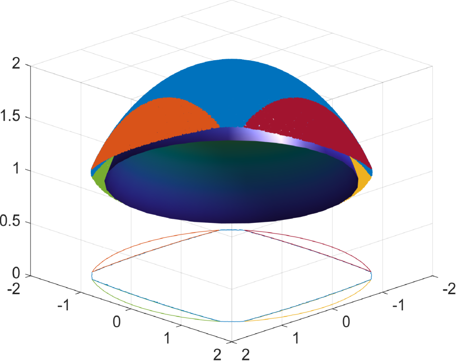
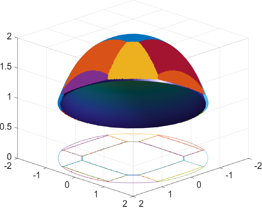
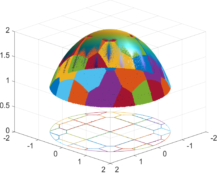
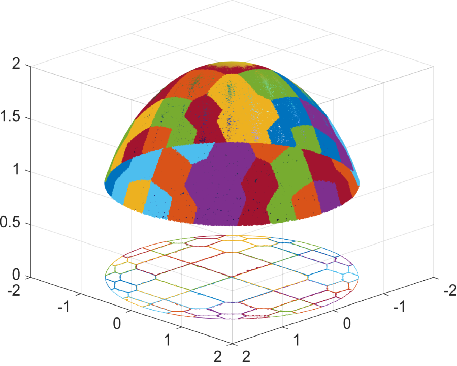
In a plane, an ellipsoid typically possesses two foci, where light emitted from one focus and reflected inside the ellipsoid converges at the second focus. To achieve the desired illumination of each point on the target, we define an ellipsoid of revolution with one focus located at the light source and the other focus positioned at the target point. However, it is important to note that for each target point, there exists an infinite number of ellipsoids of revolution that satisfy this property, differing only in their diameter. In order to achieve the desired target point density, it becomes necessary to iteratively scale the diameter of the ellipsoid. During the iteration process, the initial guess for the diameter of each ellipsoid is determined. In each iteration, the reflector is defined as the convex hull of the interior intersections of all ellipsoids. However, since the initial reflector generally does not produce the desired distribution on the target, we iteratively adjust the diameter of all ellipsoids until convergence is achieved.

The method of supporting ellipsoids produces a discrete solution for the point source reflector problem. Consider now the set $\Omega$ consists of a finite number of points and the output energy distribution on $\Omega$ is a collection of mass concentrated at these points. Based on the reflective property of the ellipsoid, we construct the reflector surface from pieces of confocal ellipsoids of revolution with the common foci at $\mathcal{O}$ and vectors defined by the points in $\Omega$ as the axes.

Figure 5.1: Discretization of uniform distribution

We obtain the discrete version of the reflector problem by representing the measure $\mu_{t}$ as a sum of Dirac measure concentrated at a finite number of points. Assume that $\Omega=\{z_{1},z_{2},\dots,z_{K}\}$ and the target distribution $\mu_{t}^{K}$ has the form

\displaystyle\mu_{t}^{K}(\omega)=\sum_{i=1}^{K}l_{i}\delta_{z_{i}}(\omega),\quad\omega\subset\Omega

(5.1)

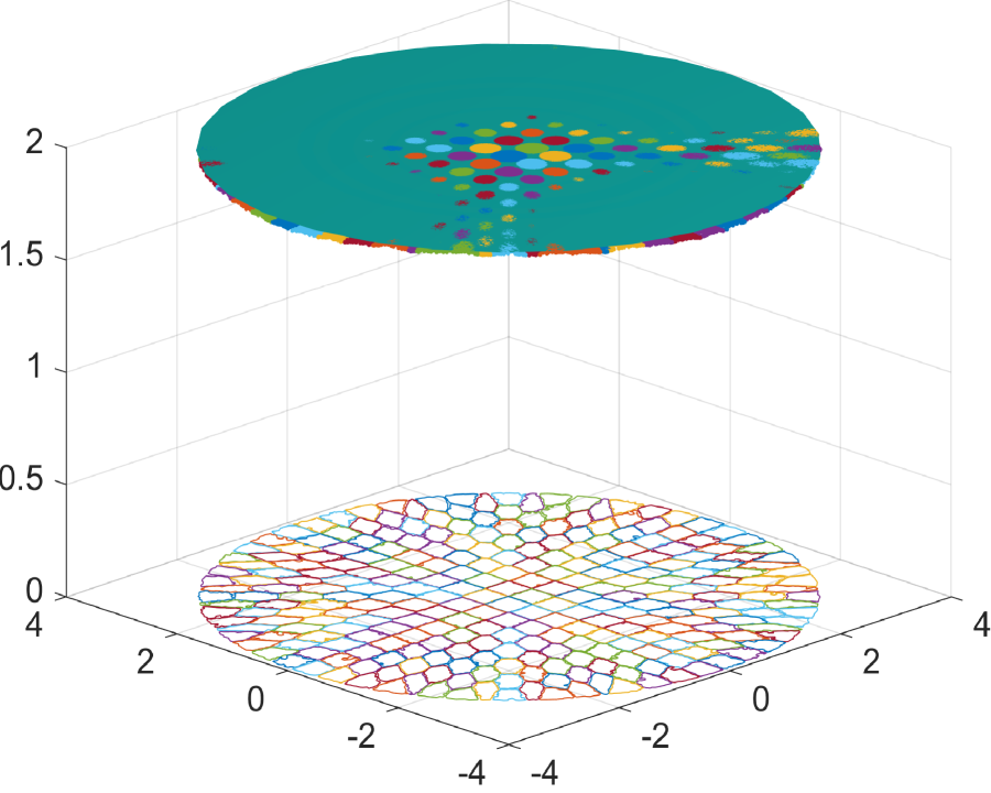
where $l_{i}$ are positive numbers, and we set

l_{i}=L(z_{i}).

Here Fig.5.1 shows the discretization of a uniform distribution on domain $\Omega$ . We assume that the mass of the set $w_{i}$ is concentrated on the point $z_{i}$ . There is $l_{1}=l_{2}=,\dots,=l_{18}=1$ . Then for each $z_{i}$ we have the corresponding visibility set $V(z_{i})$ and the corresponding measure

\displaystyle\mu_{R_{K}}(z_{i})=\int_{V(z_{i})}I(x)\,\mathrm{d}\sigma(x).

(5.2)

Let

Q\equiv\int_{\varGamma}I(m)\,\mathrm{d}\sigma(m)

and we can rewrite the energy conservation (3.4) in the form

\displaystyle Q=\sum_{i=1}^{K}l_{i}.

(5.3)

The discrete reflector problem consists in determining a reflector surface, completely defined by a finite number of ellipsoids $E_{z_{1}},E_{z_{2}},\dots,E_{z_{K}}$ , for which

\displaystyle\mu_{R_{K}}(z_{i})=l_{i},\quad\text{for}\;i=1,2,\dots,K.

(5.4)

The existence result in [20] implies that if the energy conservation condition (5.3) holds, one can construct a reflector $R_{K}$ such that

\displaystyle\frac{\sqrt{\sum_{i=1}^{K}(\mu_{R_{K}}(z_{i})-l_{i})^{2}}}{\int_{\varGamma}I(m)\,\mathrm{d}\sigma(m)}\leq\epsilon,

(5.5)

for any prescribed in advance number $\epsilon>0$ . This construction of a reflector is an important step in the proof of Theorem 4.2 because, as it was shown above, the reflector which is the weak solution to the reflector shape design problem can be obtained as a limit of this sequence of reflectors.

Let the positive integer $K>1$ and the points $z_{i}\in\Omega,i=1,2,\dots,K$ and the positive numbers $l_{i},i=1,2,\dots,K$ remain fixed. Then the reflector $R_{K}$ is completely defined by the vector $(d_{1},d_{2},\dots,d_{K})\in\mathbb{R}^{K}$ , where $d_{i}$ is the focal parameters of ellipsoids $E_{z_{i}}$ . We may identify reflector $R_{K}$ with the $(d_{1},d_{2},\dots,d_{K})$ . The $\mu_{R_{K}}$ has the following monotonicity property, which is important in constructing a reflector.

Lemma 5.1.

Let $R_{K}=(d_{1},d_{2},\dots,d_{K})$ and $R^{\prime}_{K}=(d^{\prime}_{1},d^{\prime}_{2},\dots,d^{\prime}_{K})$ be two reflectors. Suppose that some $j$ with $d_{j}\geq d^{\prime}_{j}$ , then

\mu_{R^{\prime}_{K}}(z_{j})\geq\mu_{R_{K}}(z_{j})\quad\text{and}\quad\mu_{R^{\prime}_{K}}(z_{i})\leq\mu_{R_{K}}(z_{i})\;\text{for}\;i\neq j.

For a proof of Lemma 5.1, we refer the reader to [20]. From this Lemma, the $\mu_{R_{K}}(z_{i})$ increases monotonically as $d_{i}$ decreases and by Lemma 4.1 it is continuous with respect to $d_{i}$ . Thus we can change the focal parameters of each ellipsoid to control $\mu_{R_{K}}$ so that (5.5) is satisfied in the process of constructing the reflector.

In the initial stage of the supporting ellipsoid method, total energy is collected by one ellipsoid, called the reference ellipsoid, whose focal parameter remains unchanged throughout the design process of reflector, and it determines the size of the reflector. The scale of the reflector is directly influenced by the focal parameters of the reference ellipsoid There exists a family of ellipsoids that can address the reflector shape design problem, we can ascertain a unique solution by specifying the size and geometries of the reflector. By setting these parameters, we are able to identify a unique solution within this family of ellipsoids.

We assume that the reference ellipsoid is $E_{z_{1}}$ and thus its focal parameter $d_{1}$ is fixed. Let $M=\max_{1\leq i\leq K}|z_{i}|$ , $\gamma=\max_{1\leq i\leq K}\gamma_{i}$ where $\gamma_{i}=\max_{m\in\varGamma}m\cdot\hat{z_{i}}$ and suppose that $\gamma<1$ . We have the lower and upper bounds for the focal parameters

c_{l}d_{1}<d_{i}<c_{r}d_{1}\quad\text{for}\;2\leq i\leq K,

with $c_{l}=(1-\gamma)/2$ and $c_{r}=2/(1-\gamma_{1}(\sqrt{1+d_{1}^{2}/M^{2}}-d_{1}/M))$ . In order to generate a convex reflector, all ellipsoids should initially be larger than the reference ellipsoid. Therefore all focal parameters $d_{i},\;i=2,3,\dots,K$ initially are set equal to the upper bound $c_{r}d_{1}$ . Conversely, to get a concave reflector, all focal parameters $d_{i},\;i=2,3,\dots,K$ initially are set equal to the lower bound $c_{l}d_{1}$ .

Denote by $\mathscr{R}$ the class of reflectors $R_{K}=(d_{1},d_{2},\dots,d_{K})$ with $d_{1}=\alpha M$ where $\alpha$ is a positive number, and such that

\displaystyle\mu_{R_{K}}(z_{i})\leq l_{i}+\frac{\epsilon}{K}\quad\text{for}\;i=2,3,\dots,K.

(5.6)

This inequalities (5.6) is always possible since from Lemma 5.1

\mu_{R_{K}}(z_{i})\longrightarrow 0,\;\text{as all}\;d_{2},d_{3},\dots,d_{K}\longrightarrow c_{r}d_{1},

for each $i=2,3,\dots,K$ . The implementation of the supporting ellipsoid method can be initialized with any reflector in $\mathscr{R}$ . We wish to construct a reflector $R_{K}\in\mathscr{R}$ satisfying (5.4). In order to do so, we construct a sequence of reflectors such that a) each member of the sequence is in $\mathscr{R}$ and b) the sequence monotonically converges to a solution of (5.4).

To obtain a convex reflector, we choose

\displaystyle R_{K}^{0}=(d_{1},c_{r}d_{1},\dots,c_{r}d_{1})

(5.7)

as the initial reflector for the supporting ellipsoid method. For this reflector $R_{K}^{0}$ we have

	$\displaystyle\mu_{R_{K}^{0}}(z_{1})$	$\displaystyle=Q,$
	$\displaystyle\mu_{R_{K}^{0}}(z_{i})$	$\displaystyle=0,\quad i=2,3,\dots,K,$

namely, all rays from $\mathcal{O}$ through $\varGamma$ are intercepted first by the reference ellipsoid $E_{z_{1}}$ and thus it belongs to $\mathscr{R}$ .

Then suppose that the $j$ -th element $R_{K}^{j}$ of the sequence of reflectors is constructed. To build the $R_{K}^{j+1}$ from $R_{K}^{j}$ , we iteratively scale focal parameters of each ellipsoid of reflector $R_{K}^{j}$ until the desired target distribution is produced. In the case of a convex reflector, the focal parameters are decreased, while for a reflector with concave geometry, the focal parameters are increased. By repeating the entire scaling process over, we can obtain a sequence of reflectors $\{R_{K}^{1},R_{K}^{2},\dots\}$ which ultimately converges to a solution of (5.4) that achieves the desired density at each target point. The steps of the supporting ellipsoid method for a reflector with convex geometry are summarized in Algorithm 1 [21, 9].

Algorithm 1 Supporting ellipsoid method for constructing reflectors

1:Number

K

and points

\{z_{i}\in\Omega,i=1,2,\dots,K\}

2:A sequence of reflectors

\{R_{K}^{1},R_{K}^{2},\dots\}

3:Choose an initial reflector

R_{K}^{0}=(d_{1}^{0},d_{2}^{0},\dots,d_{K}^{0})\in\mathscr{R}

4:Initialize

\widetilde{R}=R_{K}^{0}

j=0

and increments

\Delta d=(0,0,\dots,0)

5:Compute measured distribution

\mu_{\widetilde{R}}=(\mu_{\widetilde{R}}(z_{1}),\mu_{\widetilde{R}}(z_{2}),\dots,\mu_{\widetilde{R}}(z_{K}))

6:while

\mu_{\widetilde{R}}

does not satisfy the condition (5.5) do

7: Let

J\subset\{2,3,\dots,K\}

be the subset of indices for which

\mu_{\widetilde{R}}(z_{i})

do not satisfy (5.6)

8: if

J

is a empty then

R_{K}^{j+1}=\widetilde{R}

and

\Delta d_{i}=d_{i}^{j}/3,\;i\in\{2,3,\dots,K\}

10: else

11:

R_{K}^{j+1}=R_{K}^{j}

and

\Delta d_{i}=\Delta d_{i}/2,\;i\in J

12: end if

13: Put

\widetilde{R}=R_{K}^{j+1}-\Delta d=(d_{1}^{j+1},d_{2}^{j+1}-\Delta d_{2},\dots,d_{K}^{j+1}-\Delta d_{K})

14: Evaluate the measured distribution

\mu_{\widetilde{R}}=(\mu_{\widetilde{R}}(z_{1}),\mu_{\widetilde{R}}(z_{2}),\dots,\mu_{\widetilde{R}}(z_{K}))

and set

j=j+1

15:end while

Remark 5.1.

i)

The Algorithm 1 can produce a class of convex reflectors that converge to a solution of (5.4). For reflectors with concave geometry, the negative increments must be instead of positive increments and the starting point should be set

$R_{K}^{0}=(d_{1},c_{l}d_{1},\dots,c_{l}d_{1})$

and obviously $R_{K}^{0}\in\mathscr{R}$ since all energy is collected by the reference ellipsoid.
ii)

Let $\iota$ be the time to compute the integral of $\mu_{R_{K}}$ over a visibility set. Given an arbitrary error bound $\epsilon$ , the time to construct a reflector using the supporting ellipsoid method is like $O(\iota\frac{K^{4}}{\epsilon}log(\frac{K^{2}}{\epsilon}))$ [21].

For the Algorithm 1, we must evaluate the actual target distribution multiple times during each cycle. The speed of the supporting ellipsoid method and the accuracy of the results are largely driven by the computational efficiency of the target distribution estimation method. From the (5.2), we need know the visibility set $V(z_{i})$ for computing the $\mu_{R_{K}}(z_{i})$ for each $z_{i}$ . However, calculating the exact intersection of multiple ellipsoids is a very difficult and costly operation. The situation is even worse in higher dimensions. Instead, we use the ray tracing simulation method to evaluate the actual target distribution [30, 14].

The ray tracing simulation is a statistical method which can be used to evaluate the integral over a complicated domain. In this paper, for simplicity, we let $I$ be a uniform distribution on $\varGamma$ and $\varGamma=S^{n}_{+}$ . For each $z_{i}$ , the visibility set $V(z_{i})$ is a subset of $\varGamma$ . Given $N$ uniform samples $x_{j},j=1,2,\dots,N$ on $\varGamma$ , there are $N_{i}$ sample points falling within $V(z_{i})$ , and then the area ( $n-1$ dimensional content), denote by $\mathcal{A}(V(z_{i}))$ , can be approximated by

\displaystyle\mathcal{A}(V(z_{i}))\approx\mathcal{A}(\varGamma)\cdot\frac{N_{i}}{N},

(5.8)

where

\mathcal{A}(\varGamma)=\begin{cases}\frac{1}{2}\frac{n+1}{((n+1)/2)!}\pi^{(n+1)/2}&\text{if }n+1\;\text{is even},\vspace{10pt}\\ \frac{1}{2}\frac{2^{(n+1)}(n/2)!}{n!}\pi^{n/2}&\text{if }n+1\;\text{is odd},\end{cases}

is the area of $\varGamma$ where $n!=n(n-1)(n-2)\cdots$ , since the $\varGamma$ is set as the north hemisphere. Therefore we can evaluate the actual target distribution

$\displaystyle\mu_{R_{K}}(z_{i})$	$\displaystyle=\int_{V(z_{i})}I(x)\,\mathrm{d}\sigma(x)$
	$\displaystyle\approx\frac{\mathcal{A}(V(z_{i}))}{N_{i}}\sum_{j=1}^{N_{i}}I(x_{j})$
	$\displaystyle\approx\frac{\mathcal{A}(\varGamma)}{N}\sum_{j=1}^{N_{i}}I(x_{j}),$	(5.9)

for each $z_{1},z_{2},\dots,z_{K}$ and where $x_{1},x_{2},\dots,x_{N_{i}}$ are $N_{i}$ uniform samples on $V(z_{i})$ . (5.1) only requires to be able to compute the integrand at arbitrary point, make it easy to implement. If $N_{i}$ samples are used, it converges at the rate of $O(N_{i}^{-1/2})$ and does not depend on the dimensionality.

From (5.8) and (5.1) we must check whether each uniform sample on $\varGamma$ is within $V(z_{i})$ . For this method of supporting ellipsoids, we only need to determine the supporting ellipsoid for each uniform samples $x_{j},j=1,2,\dots,N$ . By the (4.5) and (4.6), the ellipsoid reflecting the ray is the one closet to, or away from, the source for the reflector with convex, or concave geometry, respectively. Thus, for each $x_{j}$ , we use (4.3) to calculate the distance between the source and each ellipsoid. Depending on the geometry of the reflector, the supporting ellipsoid then corresponds to either the minimum or maximum calculated radius: convex reflector

\displaystyle\rho(x_{j})=\min_{i}(\rho_{z_{i}}(x_{j})),\quad i=1,2,\dots,K,

(5.10)

and concave reflector

\displaystyle\rho(x_{j})=\max_{i}(\rho_{z_{i}}(x_{j})),\quad i=1,2,\dots,K.

(5.11)

5.2 Sampling by the reflector

Once we obtain the desired reflecting surface using the supporting ellipsoid method, we can utilize it to generate samples from the target distribution. However, it is important to note that the reflecting surface obtained through the supporting ellipsoid method is numerically discrete. Consequently, if we intend to obtain target samples $z_{j}=T(x_{j})$ using the reflection mapping, where $x_{j}$ represents uniform samples on $\varGamma$ , we must address the challenge of fitting the discontinuous reflecting surface. Fitting the discontinuous reflecting surface can introduce considerable errors, particularly due to variations in the surface normal. To mitigate these errors, we propose two sampling schemes facilitated by the reflector.

Interpolation sampling Since the reflecting surface is the convex hull of the interior intersection of a series of ellipsoids, we can use interpolation to smooth it. A ray $x_{j}$ (i.e., sample) emitted from a source with uniform density on the $\varGamma$ is reflected by the interior of a supporting ellipsoid $E_{z_{i}}$ to a point $z_{i}$ on target domain $\Omega$ . For a reflecting surface, each supporting ellipsoid $E_{z_{i}}$ is hit by $N_{i}$ rays. For every supporting ellipsoid $E_{z_{i}}$ , we take the mean of these $N_{i}$ uniform sample points

\bar{x}_{i}=\frac{1}{N_{i}}\sum_{j=1}^{N_{i}}x_{j},

and the mean of these $N_{i}$ radius

\bar{\rho}_{i}=\frac{1}{N_{i}}\sum_{j=1}^{N_{i}}\rho(x_{j}).

Then we get a set of points $S_{I}=\{\bar{x}_{i}\bar{\rho}_{i}\}_{i=1}^{K}$ on the reflecting surface. Therefore, for a new set of sample points $\{m_{i}\}$ from uniform distribution on the $\varGamma$ , we interpolate this point set $S_{I}$ to get the corresponding hitpoints $\{m_{i}\rho_{i}\}$ on the reflecting surface and then the target sample points are given by $\{T(m_{i})\}$ , where the reflection mapping

T(m_{i})=m_{i}\rho_{i}(m_{i})+y(m_{i})d(m_{i}),

namely, the equation (A.6) where the $D\rho_{i}$ is obtain by the second-order center difference. Note that the interpolation is done in spherical coordinate system. However, this Interpolation sampling may be unstable since the numerical differentiation is very sensitive regarding the difference step size.

Element sampling For each target point $z_{i}$ , due to the optics property of the ellipsoid, there will be $N_{i}$ rays emitted from the source and reflected by the supporting ellipsoid to reach it. In fact, since we use the Dirac measure to discretize the target distribution, these $N_{i}$ uniform samples on the $\varGamma$ should be reflected onto the neighbourhood $w_{i}$ of the target point $z_{i}$ instead of just point $z_{i}$ , see Fig.5.1 and Fig.1.1. For a new uniform sample $m_{i}$ on $\varGamma$ , we can know its corresponding supporting ellipsoid $E_{z_{i}}$ by (5.10) or (5.11) and get the corresponding point $z_{i}$ . Then a sample in the neighbourhood $w_{i}$ of target point $z_{i}$ is taken as its corresponding target sample point, namely

T(m_{i})=\vartheta_{i},\quad\vartheta_{i}\sim\mathcal{D}(w_{i}),

where $\mathcal{D}(w_{i})$ is a distribution on set $w_{i}$ . In this paper, we set $\mathcal{D}(w_{i})$ to be the uniform distribution on $w_{i}$ . This setup is not essential. In fact, when the target distribution is discrete as the sum of an infinite number of the Dirac measures, i.e., $K$ tends to infinity in (5.1), then the set $w_{i}$ shrinks to $z_{i}$ point. This Element sampling is stable and fast.

The proposed sampling method in this paper, which utilizes the geometric optics approximation, is highly efficient for solving Bayesian inverse problems. This efficiency stems from the fact that we only need to compute the reflecting surfaces within the reflector system. Specifically, based on the support ellipsoid method outlined in Section 5.1, it is evident that generating the desired reflecting surface requires computing the unnormalized posterior density function multiple times, specifically $K$ times, which corresponds to evaluating the forward model $K$ times. By utilizing this approach, we significantly reduce the computational burden associated with solving the Bayesian inverse problems. Instead of performing computationally intensive calculations for the entire posterior density, we focus solely on computing the reflecting surfaces, thereby streamlining the sampling method.

6 Numerical examples

This section showcases a series of numerical examples to illustrate the effectiveness of the sampler with geometric optics approximation method. The examples cover a range of scenarios, including closed-form reflecting surfaces, acoustic source localization, inverse problems related to general fractional diffusion equations, and advection-diffusion-reaction processes. By examining these diverse examples, we can gain insights into the performance and applicability of the geometric optics approximation method in various contexts.

6.1 Test examples

In this subsection, we will provide two analytical reflecting surfaces, i.e. sphere reflecting surface and flat reflecting surface, and show the performance of the geometrical optics approximation method. Refer to Appendices B and C for specific details of the derivation of analytic form reflecting surfaces.

Let $n=2$ , and then the $\Omega\subset P=\{x_{3}=h|h>0\}$ and $\varGamma\subset S^{2}_{+}$ . Assuming that the reflecting surface is a sphere sheet, i.e.,

\displaystyle R(m)=rm,\quad m\in\varGamma,

(6.1)

where $r$ is the polar radius and a positive constant. Then the density of target domain is given by

\displaystyle L(z)=\frac{hI(-\hat{z})}{\|z\|_{2}^{3}},\quad z\in\Omega,

(6.2)

and the $\Omega$ depends on the $\varGamma$ in the plane $P$ . Indeed, if $\varGamma$ is assumed to be a spherical cap on the $S^{2}_{+}$ and its height is $h_{c}$ , then the $\Omega$ is a disk with radius $h\sqrt{{1}/{(1-h_{c})^{2}}-1}$ . Therefore, given a spherical cap $\varGamma\subset S^{2}_{+}$ , the rays emitted from the source through this region with density $I$ , fall on the spherical reflecting surface $R$ satisfying (6.1) and are then reflected to a disk $\Omega$ and the density of the reflected light on $\Omega$ satisfies (6.2).

Similar to a sphere reflecting surface, assuming that the reflecting surface is flat and at a distance $h_{r}$ from the origin, then the flat reflecting surface is given by

\displaystyle R(m)=m\frac{h_{r}}{w},\quad m\in\varGamma.

(6.3)

Then the density of target domain is given by

\displaystyle L(z)=\frac{(2h_{r}+h)I(\hat{z^{\prime}})}{((2h_{r}+h)^{2}+z_{1}^{2}+z_{2}^{2})^{\frac{3}{2}}},\quad z\in\Omega,

(6.4)

where $z^{\prime}=z+2(h_{r}+h)\upsilon$ , and the $\Omega$ is in the plane $P$ and depends on the $\varGamma$ . Indeed, if $\varGamma$ is assumed to be a spherical cap on the $S^{2}_{+}$ and its height is $h_{c}$ , then the $\Omega$ is a disk with radius $(2h_{r}+h)\sqrt{{1}/{(1-h_{c})^{2}}-1}$ . Therefore, given a spherical cap $\varGamma\subset S^{2}_{+}$ , the rays emitted from the source through this region with density $I$ , fall on the flat reflecting surface $R$ satisfying (6.3) and are then reflected to a disk $\Omega$ and the density of the reflected light on $\Omega$ satisfies (6.4).

Let $h=1,r=2,h_{r}=2$ and $h_{c}=1-1/\sqrt{5}$ . We use the supporting ellipsoid method, i.e., Algorithm 1, to compute sphere and flat reflecting surfaces whose resulting target densities on a disk $\Omega$ satisfy (6.2) and (6.4), respectively.

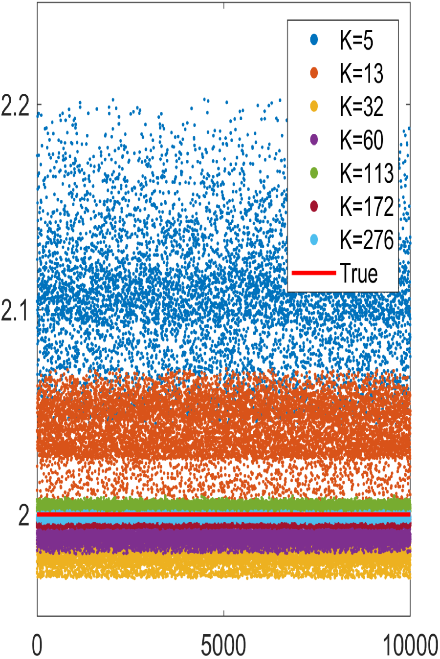
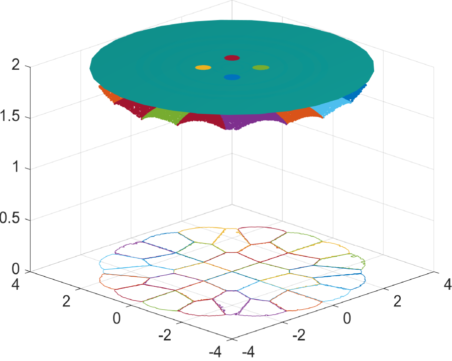
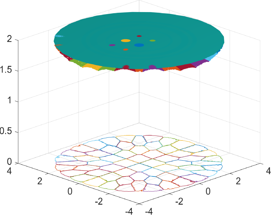
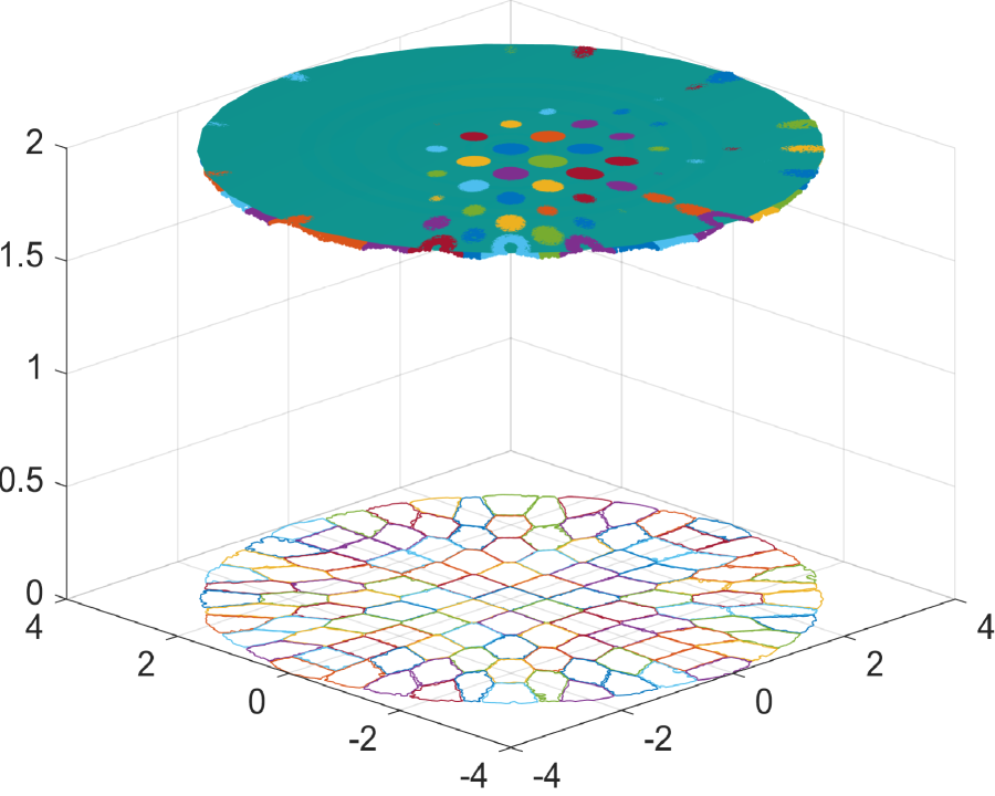
We begin by demonstrating the efficacy of the supporting ellipsoid method in constructing reflectors. Fig.6.1 showcases the results for a sphere reflecting surface, while Fig.6.2 presents the outcomes for a flat reflecting surface. As depicted in these figures, the numerical reflecting surface results obtained through Algorithm 1 progressively converge to the true reflecting surfaces as the number of ellipsoids $K$ increases. In Fig.6.1e and Fig.6.2e, we observe that the polar radius of points on the sphere and flat reflecting surfaces, as determined by the supporting ellipsoid method, gradually approaches the true polar radius as $K$ increases. This demonstrates the efficiency of constructing the reflector using the supporting ellipsoid method.

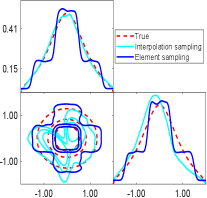
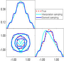
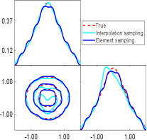
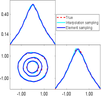
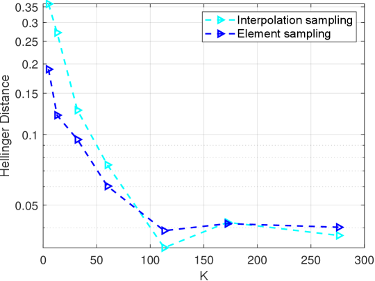
We proceed to assess the performance of interpolation sampling and element sampling techniques. Leveraging the previously obtained sphere reflecting surface, we can draw an arbitrary number of uncorrelated samples from the posterior density (6.2) using either interpolation sampling or element sampling. Fig.6.3 illustrates the marginal posterior distributions derived from interpolation sampling and element sampling. As the number of ellipsoids $K$ increases, both methods demonstrate progressively closer agreement with the true posterior density. However, element sampling exhibits a smoother convergence compared to interpolation sampling as $K$ increases. To quantitatively evaluate the agreement between the true posterior density and the estimated posterior density, we compute the Hellinger distance (more details are given in the Appendix D). Fig.6.4 presents the Hellinger distance with respect to $K$ for both interpolation sampling and element sampling. In both cases, the Hellinger distance decays rapidly as $K$ increases, consistent with the aforementioned posterior density estimation. However, when compared to interpolation sampling, element sampling exhibits a more consistent and steady decrease in the Hellinger distance. Thus, for all subsequent examples, we opt to employ element sampling for posterior distribution estimation.

6.2 Example 1: Locating acoustic source

This examples is concerned with the inverse acoustic source problem from the far field measurements for the Helmholtz system. Consider the following Helmholtz equation

\displaystyle\Delta u+k^{2}u=S\quad\text{in}\ \mathbb{R}^{2},

(6.5)

where $k>0$ is the wave number and the field $u$ satisfies the Sommerfeld Radiation Condition

\displaystyle\lim_{r\rightarrow\infty}\sqrt{r}(\frac{\partial u}{\partial r}-iku)=0,

(6.6)

where $r=\|x\|_{2},\;i=\sqrt{-1}$ , and the source

S=\lambda\delta_{z},

where $z$ is points in $\Omega$ and $\lambda\neq 0$ is scalar quantities. The solution to the (6.5) and (6.6) is formally formulated as

u(x)=-\lambda\Phi(x,z),

where

\Phi(x,y)=\frac{i}{4}H^{(1)}_{0}(k|x-y|),

is the fundamental solution to the Helmholtz equation and $H^{(1)}_{0}$ is Hankel function of the first kind of order $0$ . By the asymptotic behavior of $\Phi$ , we obtain the far field pattern

\displaystyle u_{\infty}(\hat{x})=-\frac{e^{i\frac{\pi}{4}}}{\sqrt{8\pi k}}\lambda e^{-ik\hat{x}\cdot z}\quad\hat{x}\in S^{1}.

(6.7)

The inverse acoustic source problem is to determine the locations $z$ from measurements of the far field [22, 8, 6].

In this example, we take $\lambda=1$ , $k=1$ , and the number of direction of discretization is $200$ . The exact location of acoustic source in (6.5) is set $z=(0.4,0.7)$ . The Gaussian prior $\mu_{0}$ is taken by zero mean and $[0.25\,0;0\,0.25]$ covariance matrix. The measurement data are obtained by $y=\mathcal{G}(z)+\eta$ where $\mathcal{G}$ is the far field pattern (6.7) and $\eta$ is the Gaussian noise with the standard deviation taken by $5\%,10\%,15\%$ (i.e., noise level) of the maximum norm of the model output.

In this study, we adopt a value of $\epsilon=10^{-5}$ in Algorithm 1 for all the examples presented. To discretize the target distribution on $\Omega$ , we initially sample points from the prior distribution. By computing the sample target density, we explore a domain with a target density exceeding $\epsilon$ . Subsequently, we divide the domain uniformly. It is worth emphasizing that sampling of target density includes the forward model evaluations. The results obtained through MCMC simulation serve as our reference or ‘true’ solution. For the MCMC method, we maintain an acceptance rate between $20\%$ and $30\%$ , while keeping other parameters consistent with our proposed GOAM. To evaluate the sampling performance of our GOAM, we employ the effective sample size (ESS), which measures the efficiency of the generated samples. Additionally, we utilize the Hellinger distance to quantify the discrepancy between the densities obtained by GOAM and MCMC. Further details on the evaluation of ESS and Hellinger distance can be found in Appendix D.

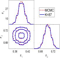
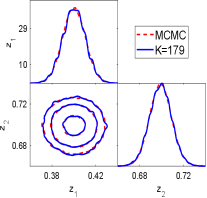
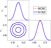
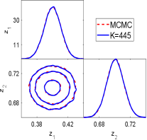
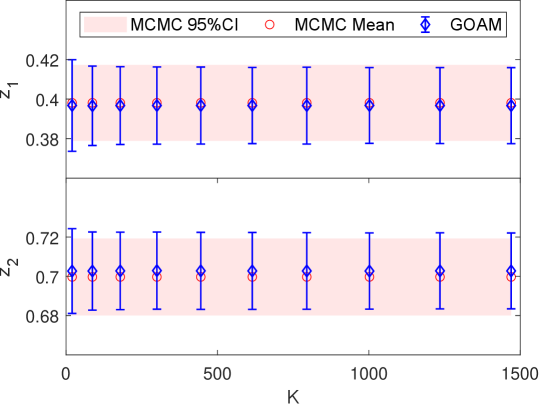
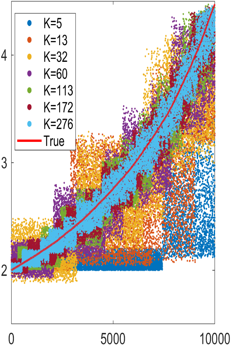
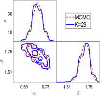
We first show the performance of the geometric optics approximation method. Fig.6.5 show the one and two dimension marginal posterior distributions estimated by the GOAM with varying $K$ at $10\%$ noise level. At $K=179$ , a good agreement with the ‘true’ solution (MCMC results) is observed, and this agreement is further improved at $K=300,445$ . However, a small number of ellipsoids ( $K=87$ ) results in a poor density estimate. Thus, the larger $K$ is, the closer the posterior density estimate obtained by the geometric optics approximation method is to the true posterior. We have shown in Fig.6.6 the samples mean and $95\%$ confidence interval given by MCMC and GOAM with respect to $K$ at $10\%$ noise level. It can be seen that the mean and confidence intervals obtained by GOAM are consistent with the ‘true’ ones, and do not depend on $K$ . Since the discrete distribution (5.1) is a good approximation of the posterior distribution.

Table 6.1: Example 1. Samples mean and standard deviation (Std) given by GOAM with

K=179

and MCMC for different noise level.

Noise Level	MCMC		GOAM
Noise Level	Mean	Std	Mean	Std
5%	(0.4016, 0.7009)	(0.0050, 0.0050)	(0.4016, 0.7009)	(0.0050, 0.0050)
10%	(0.3966, 0.7028)	(0.0100, 0.0099)	(0.3967, 0.7027)	(0.0100, 0.0101)
15%	(0.4006, 0.7003)	(0.0150, 0.0150)	(0.4006, 0.7001)	(0.0152,0.0152)

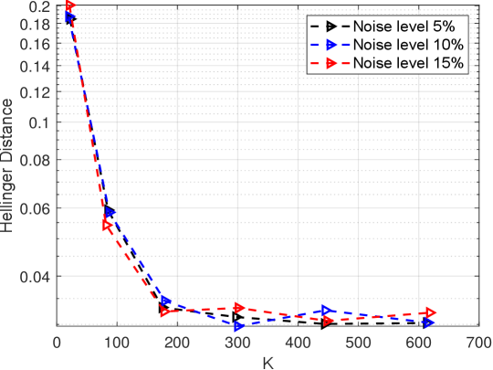
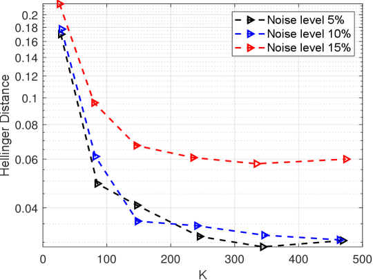
Next we investigate the stability of the reconstruction results obtained by the geometric optics approximation method. Fig.6.7 shows the Hellinger distance between posterior densities given by MCMC and GOAM with respect to $K$ for $5\%,10\%,15\%$ noise level. It can be found that as $K$ increases, it decays rapidly, which is consistent with the above Fig.6.5. Also, it can be seen that, the Hellinger distance is closer to $0$ at a smaller noise level. In addition, the posterior samples obtained by GOAM have a mean that converges to the true solution and a standard deviation that decreases with the noise level reducing, which are consistent with those given by MCMC, refer to Table 6.1. Therefore, the reconstruction results obtained by the geometric optics approximation method are stable with respect to the measurement data.

Table 6.2: Example 1. Computational time in seconds and number of forward model evaluations given by MCMC and GOAM methods at the same ESS.

Method	Offline		Online		Total(s)
Method	model evaluation( $\sharp$ )	CPU(s)	model evaluation( $\sharp$ )	CPU(s)	Total(s)
MCMC	-	-	$4.6\times 10^{6}$	132.8	132.8
GOAM_K=20	$1.01\times 10^{4}$	1.461	-	0.1065	1.567
GOAM_K=87	$1.04\times 10^{4}$	19.96	-	0.1015	20.06
GOAM_K=179	$1.09\times 10^{4}$	97	-	0.1032	97.1

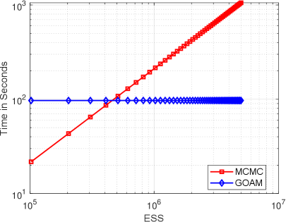
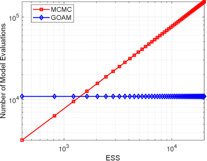
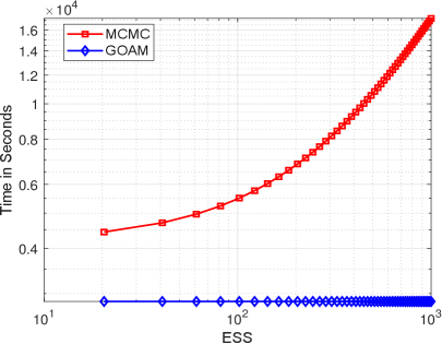
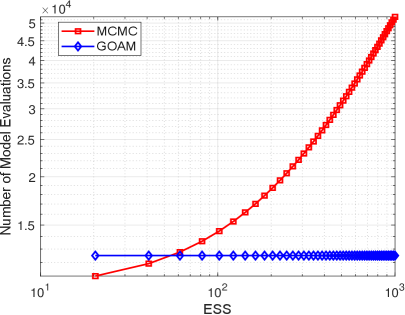
Finally we explore the sampling efficiency of the geometric optics approximation method. The computational time in seconds and the number of forward model evaluations given by MCMC and GOAM approaches at the same effective sample size, i.e., $6\times 10^{5}$ , are presented in Table 6.2. The main computational time in the geometric optics approximation method is the offline reflecting surface reconstruction. The number of such model evaluations for GOAM with $K=20,87,179$ are $1.01\times 10^{4},1.04\times 10^{4}$ and $1.09\times 10^{4}$ , respectively. Upon obtaining the reflecting surface, the online sampling is very cheap as it does not require any forward model evaluations. However, for MCMC simulations, a large number of, $4.6\times 10^{6}$ , forward models need to be computed to achieve the same ESS. Furthermore, comparing to MCMC, the computational time and number of forward model evaluations for geometric optics approximation method do not depend on the ESS, see Fig.6.8. The time and number of forward model evaluations required by the MCMC grows linearly with the ESS. On the other hand, the GOAM required a fixed amount of time or number of forward model evaluations at the beginning. If the desired number of samples is smaller and forward model is easy to compute, then MCMC is faster; otherwise the GOAM is more efficient. Nota that Fig.6.8 is drawn at $K=179$ . According to the above showing, the samples mean and standard deviation do not depend on $K$ . If one is only interested in samples mean and standard deviation, then our geometric optics approximation method with small $K$ is the most efficient, refer to Table 6.2.

6.3 Example 2: Determining fractional orders for time-space fractional diffusion equation

Nonlocal equations appear in a very natural way in the description of a wide variety of physical phenomena such as viscoelasticity, porous media, and quantum mechanics. This example considers the problem of determining the fractional order of the derivative in diffusion equation. Consider the following general nonlocal diffusion equation

$\displaystyle_{0}^{C}D^{\alpha}_{t}u$	$\displaystyle=c\frac{\partial^{\beta}u}{\partial\|x\|^{\beta}}+f\quad\text{in}\;\Omega\times(0,T),$	(6.8)
$\displaystyle u$	$\displaystyle=0\quad\text{on}\;\partial\Omega\times(0,T),$	(6.9)
$\displaystyle u\|_{t=0}$	$\displaystyle=0\quad\text{in}\;\Omega,$	(6.10)

where $c$ is the diffusion coefficient, $T>0$ is a final time and $f$ is a given function. Here ${}_{0}^{C}D^{\alpha}_{t}$ is the Caputo fractional derivative with respect to time variable $t$ [5], which is defined as

{}_{a}^{C}D^{\alpha}_{t}u=\frac{1}{\Gamma(m-\alpha)}\int_{a}^{t}\frac{\partial u(x,\xi)}{\partial\xi}\frac{\,\mathrm{d}\xi}{(t-\xi)^{\alpha-m+1}},

where $m-1<\alpha\leq m,m\in\mathbb{N}$ . And $\partial^{\beta}/\partial|x|^{\beta}$ is a partial symmetric Riesz derivative with respect to spatial variable $x$ , which is defined as a half-sum of the left- and right- sided Riemann-Liouville derivatives [25, 26]

\frac{\partial^{\beta}u}{\partial|x|^{\beta}}=\frac{1}{2}(_{a}D^{\beta}_{x}u(x)+\rule{0.0pt}{0.0pt}_{x}D^{\beta}_{b}u(x)),

where the left- and right-sided Riemann-Liouville derivatives are defined by

{}_{a}D^{\beta}_{x}u(x)=\frac{1}{\Gamma(m-\beta)}(\frac{\,\mathrm{d}}{\,\mathrm{d}x})^{m}\int_{a}^{x}\frac{u(\xi)\,\mathrm{d}\xi}{(x-\xi)^{(\beta-m+1)}},

and

{}_{x}D^{\beta}_{b}u(x)=\frac{1}{\Gamma(m-\beta)}(-\frac{\,\mathrm{d}}{\,\mathrm{d}x})^{m}\int_{x}^{b}\frac{u(\xi)\,\mathrm{d}\xi}{(\xi-x)^{(\beta-m+1)}},

where $m-1<\beta\leq m,m\in\mathbb{N}$ . The order $\alpha\in(0,1]$ and $\beta\in(0,2]$ . For $\alpha=1$ and $\beta=2$ , the equation (6.8) becomes the classical diffusion equation. The inverse problem is to determine both orders $\alpha$ and $\beta$ of fractional time and space derivatives in diffusion equations by means of the measurements data $u(x_{0},t),0<t<T$ ( $x_{0}\in\Omega$ is given). The uniqueness result for this problem has been studied in [31].

In the numerical simulation, we shall use a matrix approach [26, 27] to solve the equation (6.8)-(6.10). We take $T=0.05,\;\Omega=[0,1],\;c=1$ and $f(x,t)=8$ . The number of spatial and time steps of discretization is set $101$ and $21$ , respectively. The exact fractional orders of the derivative in (6.8) are set $\alpha=0.7$ and $\beta=1.8$ . The Gaussian prior $\mu_{0}$ is taken by $(1,1)$ mean and $[0.25\,0;0\,1]$ covariance matrix. The measurement data are obtained by $y=\mathcal{G}(\alpha,\beta)+\eta$ where $\mathcal{G}$ is the forward model (6.8)-(6.10) and $\eta$ is the Gaussian noise with the standard deviation taken by $5\%,10\%,15\%$ (i.e., noise level) of the maximum norm of the model output $u(0.1,t)$ . Notice that, in order to avoid ‘inverse crimes’, we generate measurement data by solving the forward problem on a finer grid.

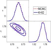
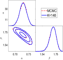
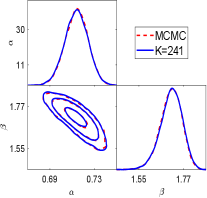
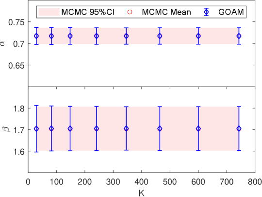
We first show the performance of the geometric optics approximation method for this example. Fig.6.9 show the one and two dimension marginal posterior distributions estimated by the GOAM with varying $K$ at $10\%$ noise level. At $K=148$ , a good agreement with the ‘true’ posterior (MCMC results) is observed, and this agreement is further improved at $K=241$ . A small number of ellipsoids ( $K=29,82$ ), however, yield a poor density estimate. Thus, the larger $K$ is, the closer the posterior density estimate obtained by the geometric optics approximation method is to the true posterior. We have shown the samples mean and $95\%$ confidence interval given by MCMC and GOAM with respect to $K$ at $10\%$ noise level in Fig.6.10. Similar to Example $1$ in section 6.2, it can be found that the mean and confidence intervals obtained by GOAM are consistent with the ‘true’ ones, and do not depend on $K$ . Because the discrete distribution (5.1) gives a good approximation to the posterior distribution.

Table 6.3: Example 2. Samples mean and standard deviation given by GOAM with

K=241

and MCMC for different noise level.

Noise Level	MCMC		GOAM
Noise Level	Mean	Std	Mean	Std
5%	(0.6972, 1.7786)	(0.0051, 0.0211)	(0.6972, 1.7788)	(0.0052, 0.0214)
10%	(0.7172, 1.7041)	(0.0097, 0.0522)	(0.7171, 1.7053)	(0.0097, 0.0525)
15%	(0.7268, 1.6678)	(0.0172, 0.1266)	(0.7261, 1.6789)	(0.0165, 0.1106)

Next we investigate the stability of the inversion results obtained by the geometric optics approximation method. Fig.6.11 shows the Hellinger distance between posterior densities given by MCMC and GOAM with respect to $K$ for $5\%,10\%,15\%$ noise level. It can be seen that it decays rapidly with $K$ increasing, which is consistent with the above Fig.6.9. It can also be observed that the Hellinger distance is closer to $0$ at a smaller noise level $5\%$ . In addition, Table 6.3 lists the samples means and standard deviations. From this table, as noise level reduce, the posterior samples obtained by GOAM have a mean that converges to the true solution and a decreasing standard deviation, and are agreement with those given by MCMC. Thus, the reconstruction results given by the geometric optics approximation method are stable with respect to the measurement data.

Finally we also explore the sampling efficiency of the geometric optics approximation method for this example. Fig.6.12 shows that the computational time in seconds and number of forward model evaluations given by GOAM with $K=241$ and MCMC simulation with respect to the ESS. The time and number of forward model evaluations required by the GOAM are fixed amounts, while the MCMC increases with the ESS. Since there is no intersection in the curves of Fig.6.12a, for this example our geometric optics approximation method, comparing to MCMC, is more efficient. Furthermore, similar to Example in section 6.2, the samples mean and standard deviation do not depend on $K$ . If one is only interested in these two statistics, then our method with small $K$ is further more efficient.

6.4 Example 3: Simultaneous reconstruction of multi-parameters in nonlinear advection-diffusion-reaction model

In this subsection, we address an inverse problem governed by a time-dependent advection-diffusion-reaction (ADR) model with a simple cubic reaction term. Our goal is to jointly infer the unknown diffusion coefficient field and the unknown initial condition field. We consider the advection-diffusion-reaction initial-boundary value problem

$\displaystyle\frac{\partial u}{\partial t}+\nu\cdot\nabla u-\nabla\cdot(m_{d}\nabla u)+cu^{3}$	$\displaystyle=f\quad\text{in}\;\Omega\times(0,T),$	(6.11)
$\displaystyle\frac{\partial u}{\partial n}$	$\displaystyle=0\quad\text{on}\;\partial\Omega\times(0,T),$	(6.12)
$\displaystyle u\|_{t=0}$	$\displaystyle=m_{0}\quad\text{in}\;\Omega,$	(6.13)

where $n$ is unit normal of $\partial\Omega$ , and $m_{d}\in L^{2}(\Omega)$ and $m_{0}\in L^{2}(\Omega)$ are the diffusion coefficient and initial field, respectively. The $\nu$ is advection velocity field, $c$ is the reaction coefficient and $f$ is the source term. It is clear that the forward problem (6.11) is nonlinear. The inverse problem is to determine both the diffusion coefficient filed and initial condition field $(m_{d},m_{0})$ in ADR model by means of the measurements data $u(x,T),x\in\Omega$ [13].

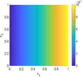
In the numerical simulation, we shall use the finite element method with Newton iteration to solve the equation (6.11)-(6.13). We take $T=0.005,\;\Omega=[0,1]\times[0,1],\;c=1,\;\nu=(cos(t),sin(t))$ and

f(x,t)=\exp\biggl{(}\frac{\|x-0.5\|_{2}^{2}}{0.9^{2}}\biggr{)}.

The number of time steps of discretization is $21$ and the $\Omega$ is discretised into a triangular mesh with $328$ elements and $185$ vertices. Let $x=(x_{1},x_{2})$ and the basis of space $L^{2}(\Omega)$ is truncated as $\{x_{1},x_{2},x_{1}^{2},x_{1}x_{2},x_{2}^{2},\dots,x_{1}^{\mathbb{K}},x_{1}^{\mathbb{K}-1}x_{2},\dots,x_{2}^{\mathbb{K}}\},$ where $\mathbb{K}$ is a positive integer. For computational simplicity, in this example we will reconstruct the coefficients of $(m_{d},m_{0})$ in this polynomial basis. The exact diffusion coefficient filed and initial condition field in (6.11) are set

m_{0}(x)=0.1x_{1}^{2}+0.2x_{1}+0.3x_{2},\quad m_{d}(x)=0.01x_{1},

respectively. The Gaussian prior $\mu_{0}$ is taken by zero mean and $[0.008\,0\,0\,0;0\,0.08\,0\,0;0\,0\,0.15\,0;$ $0\,0\,0\,0.25]^{2}$ covariance matrix. The measurement data are obtained by $y=\mathcal{G}(m_{d},m_{0})+\eta$ where $\mathcal{G}$ is the forward model (6.11)-(6.13) and $\eta$ is the Gaussian noise with the standard deviation taken by $5\%$ (i.e., noise level) of the maximum norm of the model output $u(x,T)$ . Notice that, in order to avoid ‘inverse crimes’, we generate measurement data by solving the forward problem on a finer grid.

Table 6.4: Example 3. Computational time in hours and number of forward model evaluations given by GOAM and MCMC.

Method	Offline		Online		Total(h)
Method	model evaluation( $\sharp$ )	CPU(h)	model evaluation( $\sharp$ )	CPU(h)	Total(h)
MCMC	-	-	$3\times 10^{5}$	10.25	10.25
GOAM	$2\times 10^{4}$	0.8141	-	0	0.8141

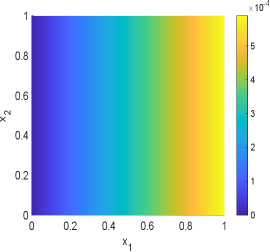
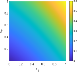
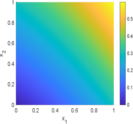
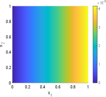
In this example, we choose $K=211$ in the geometric optics approximation method. The samples mean and standard deviation obtained by GOAM and MCMC for the inversion field $(m_{d},m_{0})$ are shown in Fig.6.13 and Fig.6.14. It can be seen that the initial condition field given by GOAM $m_{0}$ is very close to the true field and agrees with the MCMC results. However, GOAM with $K=211$ yields a poor estimate for the diffusion coefficient field $m_{d}$ , but it is in general agreement with the results of MCMC. And, the samples standard deviation obtained by GOAM and MCMC are approximately the same. The computational time in hours and number of forward model evaluations given by GOAM and MCMC are listed in Table 6.4. As we have seen, for this example, our method GOAM is about $12$ times faster than MCMC while maintaining consistent accuracy. This again confirms the efficiency of the geometric optics approximation method.

7 Conclusions

In this work, we present a novel sampling method with the geometric optics approximation for Bayesian inverse problems. This sampling method is based on the reflector shape design problem, which is concerned with constructing a reflecting surface such that rays from a source with some density is reflected off to the target domain and creates a prescribed in advance density. For our sampler, we set the density on the target domain to be the unnormalized Bayesian posterior. The distribution on the target domain for the geometric optics approximation method does not require the normalization constant but energy conservation with the source distribution. Then we define a geometric optics approximation measure for the Bayesian posterior. And we proved the well-posedness of this measure. Hence if such a reflecting surface is obtained, we can use this reflector to draw an arbitrary number of independent and uncorrelated samples from the posterior measure, completely circumventing the need for computationally intensive MCMC simulations. In order to construct the reflecting surface, we use the method of supporting ellipsoids, which stems from the constructive proof of the existence of the weak solution to the reflector shape design problem. Through some numerical examples, we demonstrate the efficiency and robustness of our novel sampler utilizing the geometric optics approximation method. It becomes evident that our sampling method outperforms MCMC, particularly in terms of efficiency.

Nevertheless, there are potential avenues for further improvement of our sampling method. The computational cost of our sampler primarily relies on determining the desired reflector. In the case of the supporting ellipsoid method, the calculation of the actual target density is required. To mitigate this computational burden, alternative and more efficient techniques can be employed to compute the intersection of surfaces, such as the target flux estimation method proposed in [4]. Furthermore, other approaches can be explored to solve the reflector shape design problem, such as solving the Monge-Ampère type differential equation [1].

An intriguing extension of our current work involves leveraging the sampler with geometric optics approximation method to accelerate MCMC simulations. By incorporating the efficient sampling technique we have developed, it is possible to enhance the performance and speed of MCMC algorithms. In addition, another natural extension of this work is to tackle high-dimensional Bayesian inverse problems. In such cases, it becomes necessary to utilize numerical methods, such as the high-dimensional support ellipsoid method, to construct reflector in higher dimensions.

Acknowledgment: The work described in this paper was supported by the NSF of China (12271151) and NSF of Hunan (2020JJ4166).

Appendix A Proof of Theorem 3.1

Proof.

Let the reflection mapping $T=(Ts,T_{n+1})$ , and denote $T_{i,j}=\partial_{j}T_{i},i=1,2,\dots,n+1,\text{and}\,j=1,2,\dots,n$ . Let $\eta=(0,0,\dots,1)$ denote the unit normal vector of $\Omega$ . We get the Jacobian determinant of $T$

$\displaystyle\det(J(T))$	$\displaystyle=\frac{(\partial_{1}T(m)\times\partial_{2}T(m)\times\cdots\times\partial_{n}T(m))\cdot\eta}{\sqrt{det(e_{ij})}}$
	$\displaystyle=w\begin{vmatrix}T_{1,1}&T_{1,2}&\ldots&T_{1,n}&\eta_{1}\\ T_{2,1}&T_{2,2}&\ldots&T_{2,n}&\eta_{2}\\ \vdots&\vdots&\ddots&\vdots&\vdots\\ T_{n,1}&T_{n,2}&\ldots&T_{n,n}&\eta_{n}\\ T_{n+1,1}&T_{n+1,2}&\ldots&T_{n+1,n}&\eta_{n+1}\\ \end{vmatrix}$
	$\displaystyle=w\begin{vmatrix}T_{1,1}&T_{1,2}&\ldots&T_{1,n}\\ T_{2,1}&T_{2,2}&\ldots&T_{2,n}\\ \vdots&\vdots&\ddots&\vdots\\ T_{n,1}&T_{n,2}&\ldots&T_{n,n}\\ \end{vmatrix}$
	$\displaystyle=:w\det(DTs).$	(A.1)

From the (3.5) and using the orthonormal coordinate system (3.6), we obtain the unit normal vector of $R$

\displaystyle\upsilon=\frac{(D\rho,0)-m(t\cdot D\rho+\rho)}{\sqrt{\rho^{2}+\|D\rho\|_{2}^{2}-(t\cdot D\rho)^{2}}},

(A.2)

Then

m\cdot\upsilon=-\frac{\rho}{\sqrt{\rho^{2}+\|D\rho\|^{2}_{2}-(D\rho\cdot m)^{2}}}.

Hence, the reflection direction is

$\displaystyle y$	$\displaystyle=m-2(m\cdot\upsilon)\upsilon$
	$\displaystyle=m+\frac{2\rho((D\rho,0)-m(\rho+D\rho\cdot m))}{\rho^{2}+\\|D\rho\\|^{2}_{2}-(D\rho\cdot m)^{2}}$
	$\displaystyle=m\frac{\\|D\rho\\|^{2}_{2}-(\rho+D\rho\cdot m)^{2}}{\rho^{2}+\\|D\rho\\|^{2}_{2}-(D\rho\cdot m)^{2}}+\frac{2\rho(D\rho,0)}{\rho^{2}+\\|D\rho\\|^{2}_{2}-(D\rho\cdot m)^{2}}.$	(A.3)

Since $\Omega\subset P$ and (1.4), we have

\displaystyle m_{n+1}\rho+y_{n+1}d=h

and from (A),

\displaystyle y_{n+1}=m_{n+1}\frac{\|D\rho\|^{2}_{2}-(\rho+D\rho\cdot m)^{2}}{\rho^{2}+\|D\rho\|^{2}_{2}-(D\rho\cdot m)^{2}},

(A.4)

therefore,

\displaystyle d=\biggl{(}\frac{h}{w}-\rho\biggr{)}\frac{\rho^{2}+\|D\rho\|^{2}_{2}-(D\rho\cdot m)^{2}}{\|D\rho\|^{2}_{2}-(\rho+D\rho\cdot m)^{2}}.

(A.5)

By (1.4),(A) and (A.5), we get

\displaystyle T=\frac{-2\rho^{2}(D\rho,0)}{\|D\rho\|^{2}_{2}-(\rho+D\rho\cdot m)^{2}}+\biggl{(}m-\frac{2\rho(D\rho,0)}{\|D\rho\|^{2}_{2}-(\rho+D\rho\cdot m)^{2}}\biggr{)}\frac{h}{w}.

(A.6)

Then

\displaystyle Ts=\frac{2Du}{\|Du\|^{2}_{2}-(u-Du\cdot t)^{2}}+\biggl{(}t-\frac{2uDu}{\|Du\|^{2}_{2}-(u-Du\cdot t)^{2}}\biggr{)}\frac{h}{w}.

(A.7)

Consider a general mapping $Q$ from $\Omega_{\varGamma}\times\mathbb{R}\times\mathbb{R}^{n}$ into $\mathbb{R}^{n}$ , and denote points in $\Omega_{\varGamma}\times\mathbb{R}\times\mathbb{R}^{n}$ by $(x,r,p)$ , we see from (A.7)

	$\displaystyle Q(x,r,p)$	$\displaystyle=\frac{2p}{\\|p\\|^{2}_{2}-(r-p\cdot x)^{2}}+\biggl{(}x-\frac{2rp}{\\|p\\|^{2}_{2}-(r-p\cdot x)^{2}}\biggr{)}\frac{h}{w}$
		$\displaystyle:=Y+W,$		(A.8)

and then

$\displaystyle DTs$	$\displaystyle=DQ$
	$\displaystyle=Q_{p}D^{2}u+Q_{x}+Q_{r}\otimes Du$
	$\displaystyle=(Y_{p}+W_{p})\bigl{[}D^{2}u+(Y_{p}+W_{p})^{-1}(Y_{x}+Y_{r}\otimes Du+W_{x}+W_{r}\otimes Du)\bigr{]}$
	$\displaystyle:=(Y_{p}+W_{p})\bigl{[}D^{2}u+A(\cdot,r,p)\bigr{]}.$	(A.9)

By (3.2), (A) and (A), we then have

\displaystyle\Bigl{|}\det\bigl{[}D^{2}u+A(\cdot,r,p)\bigr{]}\Bigr{|}=\frac{1}{\bigl{|}\det[Y_{p}+W_{p}]\bigr{|}}\cdot\frac{I}{wL\circ T}.

(A.10)

For $Y=Y(x,r,p)$ in (A), it is easy to compute that

\displaystyle Y_{x}+Y_{r}\otimes Du=0,

(A.11)

and

\displaystyle Y_{p}=\frac{2}{\|p\|^{2}_{2}-(r-p\cdot t)^{2}}\Biggl{[}Id-\frac{2p\otimes\bigl{[}p+(r-p\cdot t)t\bigr{]}}{\|p\|^{2}_{2}-(r-p\cdot t)^{2}}\Biggr{]}.

(A.12)

Similarly,

\displaystyle W_{x}+W_{r}\otimes Du=cId+\frac{ct\otimes t}{1-\|t\|^{2}_{2}}-\frac{2c}{\|p\|^{2}_{2}-(r-p\cdot t)^{2}}(\frac{rp\otimes t}{1-\|t\|^{2}_{2}}+p\otimes p),

(A.13)

and

\displaystyle W_{p}=-crY_{p}.

(A.14)

Hence,

\displaystyle Y_{p}+W_{p}=\frac{2(1-cr)}{a}\Biggl{[}Id-\frac{2p\otimes\bigl{[}p+(r-p\cdot t)t\bigr{]}}{a}\Biggr{]}.

(A.15)

Using the formula $\det[Id+\alpha\otimes\beta]=1+\alpha\cdot\beta$ and $(Id+\alpha\otimes\beta)^{-1}=Id-\alpha\otimes\beta/(1+\alpha\cdot\beta)$ for any vector $\alpha,\beta\in\mathbb{R}^{n}$ , we have

\displaystyle\det[Y_{p}+W_{p}]=-\frac{2^{n}(1-cr)^{n}b}{a^{n+1}},

(A.16)

and

\displaystyle(Y_{p}+W_{p})^{-1}=\frac{a}{2(1-cr)}\Biggl{[}Id-\frac{2p\otimes\bigl{[}p+(r-p\cdot t)t\bigr{]}}{b}\Biggr{]}.

(A.17)

Hence, by (A.11)-(A.15) and (A.17), we get

\displaystyle A(\cdot,r,p)=\frac{ca}{2(1-cr)}(1+\frac{t\otimes t}{1-\|t\|^{2}_{2}}).

(A.18)

Combining (A.10), (A.16) and (A.18), we have then obtain the equation (3.7). ∎

Appendix B Sphere reflecting surface

Let $n=2$ , and then the $\Omega\subset P=\{x_{3}=h|h>0\}$ and $\varGamma\subset S^{2}_{+}$ . Assuming that the reflecting surface is a spherical sheet, i.e.,

\displaystyle R(m)=rm,\quad m\in\varGamma,

(B.1)

where $r$ is the polar radius and a positive constant, then the direction of reflection is

y=-m.

Indeed, the unit normal direction $\upsilon$ of the reflecting surface is equal to the direction $m$ of ray emission. Then from the (1.4), the reflection mapping is given by

\displaystyle z=T(m)=-\frac{h}{w}m.

(B.2)

Hence from (3.2) and (B.2), we obtain

L(T(m))=\frac{I(m)w^{3}}{h^{2}},\quad m\in\varGamma.

Then the density of target domain is given by

\displaystyle L(z)=\frac{hI(-\hat{z})}{\|z\|_{2}^{3}},\quad z\in\Omega,

(B.3)

and the $\Omega$ is in the plane $P$ and depends on the $\varGamma$ . Indeed, if $\varGamma$ is assumed to be a spherical cap on the $S^{2}_{+}$ and its height is $h_{c}$ , then the $\Omega$ is a disk with radius $h\sqrt{{1}/{(1-h_{c})^{2}}-1}$ . And the normalisation constant of density (B.3) is given by $2\pi Ih_{c}$ if the $I$ is a uniform distribution.

Therefore, given a spherical cap $\varGamma\subset S^{2}_{+}$ , the rays emitted from the source through this region with density $I$ , fall on the spherical reflecting surface $R$ satisfying (B.1) and are then reflected to a disk $\Omega$ and the density of the reflected light on $\Omega$ is equal to $L$ satisfying (B.3).

Appendix C Flat reflecting surface

Similar to a spherical reflecting surface, assuming that the reflecting surface is flat and at a distance $h_{r}$ from the origin, then the flat reflecting surface is given by

\displaystyle R(m)=m\frac{h_{r}}{w},\quad m\in\varGamma.

(C.1)

Indeed, its unit normal direction is $\upsilon=(0,0,1)$ . The direction of reflection is

y=m-2w\upsilon.

Then from the (1.4), the reflection mapping is given by

\displaystyle z=T(m)=m\frac{2h_{r}+h}{w}-2(h_{r}+h)\upsilon

(C.2)

Hence from (3.2) and (C.2), we obtain

L(T(m))=\frac{I(m)w^{3}}{(h_{r}+h)^{2}},\quad m\in\varGamma.

Then the density of target domain is given by

\displaystyle L(z)=\frac{\sqrt{2h_{r}+h}I(\hat{z^{\prime}})}{((2h_{r}+h)^{2}+z_{1}^{2}+z_{2}^{2})^{\frac{3}{2}}},\quad z\in\Omega,

(C.3)

Therefore, given a spherical cap $\varGamma\subset S^{2}_{+}$ , the rays emitted from the source through this region with density $I$ , fall on the flat reflecting surface $R$ satisfying (C.1) and are then reflected to a disk $\Omega$ and the density of the reflected light on $\Omega$ is equal to $L$ satisfying (C.3).

Appendix D Evaluation of effective sample size and Hellinger distance

Evaluation of effective sample size Here we describe the calculation of effective sample size (ESS) used in our results. Let the $\tau_{i}$ be the integrated autocorrelation time of dimension $i$ . This value is given by

\tau_{i}=1+2\sum_{j=1}^{N_{s}}corr(\theta_{1},\theta_{1+j})

for dimension $i$ of samples $\{\theta_{j}\}_{j=1}^{N_{s}}$ , where $corr(\cdot,\cdot)$ is the correlation coefficient. Then we define the maximum integrated autocorrelation time over all dimension

\tau_{max}=\max_{i\in\{1,2,\dots,n\}}\tau_{i}

The ESS is then computed by

ESS=\frac{N_{s}}{\tau_{max}}.

Evaluation of Hellinger distance Let $\mu_{1}$ and $\mu_{2}$ be two probability measure. If they both have Radon-Nikodym derivatives $f$ and $g$ with respect to the Lebesgue measure, then the Hellinger distance is defined as

H^{2}(\mu_{1},\mu_{2})=\frac{1}{2}\int\Bigl{(}\sqrt{f(x)}-\sqrt{g(x)}\Bigr{)}^{2}\,\mathrm{d}x.

Hence,

H(\mu_{1},\mu_{2})\approx\frac{1}{\sqrt{2}}\sqrt{\sum_{i=1}^{N_{H}}\Bigl{(}\sqrt{f_{i}}-\sqrt{g_{i}}\Bigr{)}},

where $f_{i}=f(x_{i}),g_{i}=g(x_{i}),i=1,2,\dots,N_{H}$ .

References

[1] K. Brix, Y. Hafizogullari, and A. Platen. Solving the monge–ampère equations for the inverse reflector problem. Mathematical Models and Methods in Applied Sciences, 25(05):803–837, 2015.
[2] L. Caffarelli and V. I. Oliker. Weak solutions of one inverse problem in geometric optics. Journal of Mathematical Sciences, 154:39–49, 2008.
[3] L. A. Caffarelli, S. A. Kochengin, and V. I. Oliker. Problem of reflector design with given far-field scattering data. Monge Ampère equation: applications to geometry and optimization, 226:13, 1999.
[4] C. Canavesi, W. J. Cassarly, and J. P. Rolland. Target flux estimation by calculating intersections between neighboring conic reflector patches. Optics letters, 38(23):5012–5015, 2013.
[5] M. Caputo. Elasticita e dissipazione. Zanichelli, 1969.
[6] A. El Badia and T. Nara. An inverse source problem for helmholtz’s equation from the cauchy data with a single wave number. Inverse Problems, 27(10):105001, 2011.
[7] T. A. El Moselhy and Y. M. Marzouk. Bayesian inference with optimal maps. Journal of Computational Physics, 231(23):7815–7850, 2012.
[8] M. Eller and N. P. Valdivia. Acoustic source identification using multiple frequency information. Inverse Problems, 25(11):115005, 2009.
[9] F. R. Fournier, W. J. Cassarly, and J. P. Rolland. Fast freeform reflector generation using source-target maps. Optics Express, 18(5):5295–5304, 2010.
[10] V. Galindo. Design of dual-reflector antennas with arbitrary phase and amplitude distributions. IEEE Transactions on Antennas and Propagation, 12(4):403–408, 1964.
[11] V. Galindo-Israel, W. A. Imbriale, R. Mittra, and K. Shogen. On the theory of the synthesis of offset dual-shaped reflectors-case examples. IEEE transactions on antennas and propagation, 39(5):620–626, 1991.
[12] A. Gelman, J. B. Carlin, H. S. Stern, D. B. Dunson, A. Vehtari, and D. B. Rubin. Bayesian data analysis. CRC press, 2013.
[13] O. Ghattas and K. Willcox. Learning physics-based models from data: perspectives from inverse problems and model reduction. Acta Numerica, 30:445–554, 2021.
[14] A. S. Glassner. An introduction to ray tracing. Morgan Kaufmann, 1989.
[15] T. Graf and V. I. Oliker. An optimal mass transport approach to the near-field reflector problem in optical design. Inverse Problems, 28(2):025001, 2012.
[16] H. Groemer. Stability results for convex bodies and related spherical integral transformations. Advances in Mathematics, 109:45–74, 1994.
[17] P. Guan, X.-J. Wang, et al. On a monge-ampere equation arising in geometric optics. Journal of Differential Geometry, 48(2):205–223, 1998.
[18] J. Kaipio and E. Somersalo. Statistical and computational inverse problems, volume 160. Springer Science & Business Media, 2006.
[19] A. Karakhanyan and X.-J. Wang. On the reflector shape design. Journal of Differential Geometry, 84(3):561–610, 2010.
[20] S. A. Kochengin and V. I. Oliker. Determination of reflector surfaces from near-field scattering data. Inverse problems, 13(2):363, 1997.
[21] S. A. Kochengin and V. I. Oliker. Determination of reflector surfaces from near-field scattering data ii. numerical solution. Numerische Mathematik, 79(4):553–568, 1998.
[22] Y. Liu, Y. Guo, and J. Sun. A deterministic-statistical approach to reconstruct moving sources using sparse partial data. Inverse Problems, 37(6):065005, 2021.
[23] Y. Marzouk, T. Moselhy, M. Parno, and A. Spantini. Sampling via measure transport: An introduction. Handbook of uncertainty quantification, 1:2, 2016.
[24] V. I. Oliker. On reconstructing a reflecting surface from the scattering data in the geometric optics approximation. Inverse problems, 5(1):51, 1989.
[25] I. Podlubny. Fractional differential equations academic press. San Diego, Boston, 6, 1999.
[26] I. Podlubny. Matrix approach to discrete fractional calculus. Fractional calculus and applied analysis, 3(4):359–386, 2000.
[27] I. Podlubny, A. Chechkin, T. Skovranek, Y. Chen, and B. M. V. Jara. Matrix approach to discrete fractional calculus ii: Partial fractional differential equations. Journal of Computational Physics, 228(8):3137–3153, 2009.
[28] C. P. Robert, G. Casella, and G. Casella. Monte Carlo statistical methods, volume 2. Springer, 1999.
[29] J. Schruben. Formulation of a reflector-design problem for a lighting fixture. Journal of the Optical Society of America, 62(12):1498–1501, 1972.
[30] P. Shirley and R. K. Morley. Realistic ray tracing. AK Peters, Ltd., 2008.
[31] S. Tatar and S. Ulusoy. A uniqueness result for an inverse problem in a space-time fractional diffusion equation. Electronic Journal of Differential Equations, 257:1–9, 2013.
[32] L. Tierney. Markov chains for exploring posterior distributions. The Annals of Statistics, pages 1701–1728, 1994.
[33] J. I. Urbas. Regularity of generalized solutions of monge-ampere equations. Mathematische Zeitschrift, 197:365–393, 1988.
[34] C. Villani. Topics in optimal transportation, volume 58. American Mathematical Soc., 2021.
[35] C. Villani et al. Optimal transport: old and new, volume 338. Springer, 2009.
[36] X.-J. Wang. On the design of a reflector antenna. Inverse problems, 12(3):351, 1996.
[37] X.-J. Wang. On the design of a reflector antenna ii. Calculus of Variations and Partial Differential Equations, 20(3):329–341, 2004.

Bayesian inference via geometric optics approximation

1 Introduction

2 The Bayesian framework

3 Mathematical formulation of reflector shape design

Theorem 3.1.

Remark 3.1.

4 Geometric optics approximation for Bayesian inference

4.1 Geometric optics approximation measure

Definition 4.1.

Definition 4.2.

Remark 4.1.

Remark 4.2.

Remark 4.3.

Definition 4.3.

4.2 Well-posedness

Lemma 4.1.

Theorem 4.2 (Existence and uniqueness of weak solution).

Remark 4.4.

Remark 4.5.

Theorem 4.3 (Stability of reflector with respect to target domain).

Proof.

Theorem 4.4 (Stability of geometric optics approximation measure μR\mu_{R} with respect to target domain).

Proof.

5 Sampling with the geometric optics approximation method

5.1 The method of supporting ellipsoids

Lemma 5.1.

Remark 5.1.

5.2 Sampling by the reflector

6 Numerical examples

6.1 Test examples

6.2 Example 1: Locating acoustic source

6.3 Example 2: Determining fractional orders for time-space fractional diffusion equation

6.4 Example 3: Simultaneous reconstruction of multi-parameters in nonlinear advection-diffusion-reaction model

7 Conclusions

Appendix A Proof of Theorem 3.1

Proof.

Appendix B Sphere reflecting surface

Appendix C Flat reflecting surface

Appendix D Evaluation of effective sample size and Hellinger distance

References

Theorem 4.4 (Stability of geometric optics approximation measure $\mu_{R}$ with respect to target domain).