Bayesian Inference for Relational Graph in a Causal Vector Autoregressive Time Series
Abstract
We propose a method for simultaneously estimating a contemporaneous graph structure and autocorrelation structure for a causal high-dimensional vector autoregressive process (VAR). The graph is estimated by estimating the stationary precision matrix using a Bayesian framework. We introduce a novel parameterization that is convenient for jointly estimating the precision matrix and the autocovariance matrices. The methodology based on the new parameterization has several desirable properties.
A key feature of the proposed methodology is that it maintains causality of the process in its estimates and also provides a fast feasible way for computing the reduced rank likelihood for a high-dimensional Gaussian VAR. We use sparse priors along with the likelihood under the new parameterization to obtain the posterior of the graphical parameters as well as that of the temporal parameters. An efficient Markov Chain Monte Carlo (MCMC) algorithm is developed for posterior computation. We also establish theoretical consistency properties for the high-dimensional posterior. The proposed methodology shows excellent performance in simulations and real data applications.
Keywords: Graphical model; reduced rank VAR; Schur stability; sparse prior; stationary graph;
1 Introduction
Graphical models are popular models that encode scientific linkages between variables of interest through conditional independence structure and provide a parsimonious representation of the joint probability distribution of the variables, particularly when the number of variables is large. Thus, learning the graph structure underlying the joint probability distribution of a large collection of variables is an important problem and it has a long history. When the joint distribution is Gaussian, learning graphical structure can be done by estimating the precision matrix leading to the popular Gaussian Graphical Model (GGM); even in the non-Gaussian case one can think of encoding the graph using the partial correlation structure and learn the Partial Correlation Graphical Model (PCGM) by estimating the precision matrix. However, when the sample has temporal dependence, estimating the precision matrix efficiently from the sample can be challenging. If estimating the graphical structure is the main objective, the temporal dependence can be treated as a nuisance feature and ignored in the process of graph estimation. When the temporal features are also important to learn, estimating the graph structure and the temporal dependence simultaneously can be considerably more complex.
There are several formulations of graphical models for time series. A time series graph could be one with the nodes representing the entire coordinate processes. In particular, if the coordinate processes are jointly stationary, this leads to a ‘stationary graphical’ structure. Conditional independence in such a graph can be expressed equivalently in terms of the absence of partial spectral coherence between two nodal series; see Dahlhaus (2000). Estimation of such stationary graphs have been investigated by Jung et al. (2015); Fiecas et al. (2019), Basu and Rao (2023), Basu et al. (2015) and Ma and Michailidis (2016).
A weaker form of conditional coding for stationary multivariate time series is a ‘contemporaneous stationary graphical’ structure where the graphical structure is encoded in the marginal precision matrix. In a contemporaneous stationary graph, the nodes are the coordinate variables of the vector time series. If the time series is Gaussian, this leads to contemporaneous conditional independence among the coordinates of the vector time series. This is the GGM structure which has the appealing property that conditional independence of a pair of variables given the others is equivalent to the zero-value of the corresponding off-diagonal entry of the precision matrix and hence graph learning can be achieved via estimation of precision matrices. A rich literature on estimating the graphical structure can be found in classical books like Lauritzen (1996); Koller and Friedman (2009); see also Maathuis et al. (2019) and references therein for more recent results. When the distribution is specified only up to the second moment, which is common in the study of second-order stationary time series, one could learn the contemporaneous partial correlation graphical structure by estimating the stationary precision matrix. In this paper, we use the contemporaneous precision matrix of a stationary time series to estimate the graph along the line of Qiu et al. (2016); Zhang and Wu (2017). For modeling the temporal dynamics we use a vector autoregression (VAR) model.
This paper brings together two popular models: the PCGM for graph estimation and the VAR model for estimating the temporal dynamics in vector time series. However, modeling the partial correlation graph and the temporal dependence with the VAR structure simultaneously is challenging, particularly under constraints such as reduced rank and causality on the VAR model and sparsity on the graphical model. This is achieved in this paper via a novel parameterization of the VAR process. The main contribution of the paper is a methodology that allows for meeting the following two challenging objectives simultaneously:
-
(i)
Estimation of the contemporaneous stationary graph structure under a sparsity constraint.
-
(ii)
Estimation of VAR processes with a reduced rank structure under causality constraints.
A novelty of the proposed approach is that while developing the methodology for performing the above two tasks, we can
-
(a)
develop a recursive computation scheme for computing the reduced-rank VAR likelihood through low-rank updates;
-
(b)
establish posterior concentration under priors based on new parameterization.
2 Partial Correlation Graph Under Autoregression
The partial correlation graph for a set of variables can be identified by the precision matrix of , that is, the inverse of the dispersion matrix of . Two components and are conditionally uncorrelated given the remaining components if and only if the th entry of the precision matrix of is zero. Then the relations can be expressed as a graph on where and are connected if and only if and are conditionally correlated given the remaining components. Equivalently, an edge connects and if and only if the partial correlation between and is non-zero.
In many contexts, the set of variables of interest evolve over time and are temporally dependent. If the process is stationary, that is, the joint distributions remain invariant under a time-shift, the relational graph of remains time-invariant. A vector autoregressive (VAR) process provides a simple, interpretable mechanism for temporal dependence by representing the process as a fixed linear combination of itself at a few immediate time points plus an independent random error. It is widely used in time series modeling. In this paper, we propose a Bayesian method for learning the relational graph of a stationary VAR process.
Let be a sample of size from a Vector Autoregressive process of order , VAR in short, given by
| (2.1) |
where , are real matrices and is a dimensional white noise process with covariance matrix , that is, are independent . We consider to be given, but in practice, it may not be known and may have to be assessed by some selection methods.
Causality is a property that plays an important role in multivariate time series models, particularly in terms of forecasting. For a causal time series, the prediction formula includes current and past innovations, and hence a causal time series allows a stable forecast of the future in terms of present and past data. However, the condition of causality imposes complex constraints on the parameters of the process, often making it extremely difficult for one to impose causality during the estimation process. An effective approach is to parameterize the constrained parameter space of causal processes in terms of unconstrained parameters and write the likelihood and the prior distribution in terms of the unconstrained parameters.
For a VAR time series defined by (2.1), causality is determined by the roots of the determinantal equation
| (2.2) |
is the matrix polynomial associated with the VAR equation. For the VAR model to be causal, all roots of the determinantal equation must lie outside the unit disc . When the roots of the determinantal equation lie outside the unit disc, the associated monic matrix polynomial is called Schur stable. Roy et al. (2019) provided a parameterization of the entire class of Schur stable polynomials and thereby parameterized the space of causal VAR models.
For convenience, we briefly describe the Roy et al. (2019) framework. Roy et al. (2019) noted that the VAR model (2.1) is causal if and only if the block Toeplitz covariance matrix is positive definite, where
| (2.3) |
is the covariance matrix of consecutive observations and
| (2.4) |
is the lag- autocorrelation matrix of the process. As shown in Roy et al. (2019), this condition is equivalent to
| (2.5) |
where are the the conditional dispersion matrices; here and below, we use the Lowner ordering: for two matrices , means that is nonnegative definite. The condition (2.5) plays a central role in the formulation of our parameterization. Since the VAR parameters can be expressed as a one-to-one map of the sequence , the parameterization of the causal VAR process is achieved by parameterizing the nonnegative matrices of successive differences , and the positive definite matrix in terms of unconstrained parameters. Several options for parameterizing nonnegative matrices in terms of unconstrained parameters are available in the literature.
Our main objectives in this paper is to estimate the stationary precision matrix of the process, , under sparsity restrictions. In the Roy et al. (2019) parameterization, the stationary variance and hence are functions of the basic free parameters and hence not suitable for estimation of the graphical structure with desired sparsity properties. We suggest a novel modification of the previous parameterization that achieves the goal of parameterizing the graphical structure and the VAR correlation structure directly and separately, thereby facilitating the estimation of both components under the desired restrictions, even in higher dimensions.
3 Reduced Rank Parameterization and Priors
The main idea in the proposed parameterization is separation of the parameters pertaining to the graphical structure, and the parameters that are used to describe the temporal correlation present in the sample. The following result is essential in developing the parameterization. It follows easily from (2.5) but due to its central nature in the new parameterization, we state it formally.
Proposition 1.
Let satisfying (2.1) be a stationary vector autoregressive time series with stationary variance , a positive definite matrix and error covariance matrix . Then is causal if and only if
| (3.1) |
where for any .
Constraint-free parameterization: Based on Proposition 1, for a causal VAR process the successive differences are nonnegative definite for , where . Hence, these successive differences, along with the precision matrix , can be parameterized using an unrestricted parameterization that maps non-negative definite matrices to free parameters.
3.1 Efficient Computation of the Likelihood
The computation of the likelihood is difficult for a multivariate time series. For a Gaussian VAR process, the likelihood can be computed relatively fast using the Durbin-Levison (DL) or innovations algorithm. However, under different parameterizations, the computational burden can increase significantly depending on the complexity of the parameterization. Moreover, the DL-type algorithm can still be challenging if the process dimension is high.
In models with a high number of parameters, a common approach is to seek low-dimensional sub-models that could adequately describe the data and answer basic inferential questions of interest.
Using the proposed parameterization of and the differences , we provide a low-rank formulation of a causal VAR process that leads to an efficient algorithm for computing the likelihood based on a Gaussian VAR() sample. The algorithm achieves computational efficiency by avoiding inversion of large dimensional matrices. The sparse precision matrix is modeled as a separate parameter, allowing direct inference about the graphical structure under sparsity constraints . The likelihood computation requires the inversion of only matrices instead of matrices. The last fact substantially decreases the computational complexity. In particular, when , i.e. when the conditional precision updates, , are all rank-one, all components of likelihood computation can be done without matrix inversion or factorization.
Before we proceed, we define some notations that are used throughout the article. The stationary variance matrix of as defined in (2.3), will be written in the following nested structures
| (3.2) |
where
| (3.3) |
Denote the Schur-complements of in the two representations as
| (3.4) |
Also, let and denote the probability density and cumulative distribution function of the -dimensional normal with mean and covariance . The basic computation will be to successively compute the likelihood contribution of the conditional densities . Let . Under the assumption that the errors are Gaussian, i.e., , and that they are independent, and writing , , we have,
| (3.5) |
where the conditional mean and variance are given by , for any and , for . Thus, the full Gaussian likelihood
| (3.6) |
can be obtained by recursively deriving the conditional means and variances from the constraint-free parameters describing the sparse precision matrix and the reduced-rank conditional variance differences, . For parameterization of the conditional precision updates, we use a low-rank parameterization. Specifically, let
| (3.7) |
The rank factors are not directly solvable from the precision updates . To complete the parameterization, we need to define a bijection. The bijection can be defined by augmenting with semi-orthogonal matrices and define as a unique square-root of , such as the unique symmetric square-root. This would lead to an identifiable parameterization. However, given that the entries in are constrained by the orthogonality requirement, we will use a slightly over-identified system of parameters to describe the reduced rank formulation of , . The over-identification facilitates computation enormously without creating any challenges in inference for the parameters of interest.
Specifically, for each along with we will use parameters arranged in a matrix, , to describe the reduced-rank updates . The exact definition of the matrices along with the steps for computing the causal VAR likelihood based on the basic constraint-free parameters , , and , are given below. We assume the that the ranks are specified and fixed. Also, unless otherwise specified, we will assume the matrix square roots for pd matrices to be the unique symmetric square-root. Then, given the parameters and the initialization the following steps describe the remaining parameters recursively along with recursive computation of the components of the VAR likelihood.
Recursive Computation of the Reduced Rank VAR Likelihood
For
-
1.
Since we have
-
2.
Using the Sherman-Woodbury-Morrison (SWM) formula for partitioned matrices, where
(3.8) Note that,
Since for a positive definite matrix , satisfies the restriction
-
3.
Define
(3.9) with From Roy et al. (2019), and hence for any such that we have
(3.10) While are determined by , the matrices are determined by the other parameters . We construct from the basic parameters as,
(3.11) Note that .
-
4.
Thus, entries of the covariance matrices can be updated as
-
5.
Applying SWM successively, we have
where and . For the last update to hold one needs to be positive definite. This follows from the fact that :
where the final equation holds because Recalling the result follows. Thus,
-
6.
Finally, the th conditional density in the likelihood is updated as
The determinant term can be updated recursively as
The subsequent updates , required to compute the rest of the factors of the likelihood, can be obtained simply noting and where
3.2 Identification of the Parameters
In the recursive algorithm described above, the parameters are mapped to the modified parameters . The mapping is not one-to-one since each has the restriction while the basic parameters do not have any restrictions. The intermediate parameters in the mapping, , are identifiable only up to rotations. Consider the equivalence classes of pair of matrices defined through the relation for any orthogonal matrix . Let for each , be the set of such equivalence classes. Also let be a subset of the positive definite cone with specified sparsity level . The following proposition shows that there is a bijection from the set to the causal VAR parameter space defined by the VAR coefficients and innovation variance , where polynomials with coefficients satisfy low-rank restrictions and the stationary precision satisfies -sparsity. The definition of sparsity is made more clear in the prior specification section. For simplicity, we use a mean zero VAR() process. Before we formally state the identification result, we state and prove a short Lemma that is used to show identification.
Lemma 1.
Given a matrix of rank for some positive integer , and a positive definite matrix , there exists matrices and such that , and
Proof.
Given a rank factorization and the symmetric square root , let be the Q-R decomposition of where is semi-orthogonal and is nonsingular matrix. Then where and . For this choice, ∎
Proposition 2.
Let be a positive definite matrix, which is -sparse. Let , be given full column rank matrix pairs, of order , respectively. Then there is a unique causal process with stationary variance matrix and autcovariances (and hence the coefficients as the Yule-Walker solution) uniquely determined recursively from . The associated increments in the conditional precision matrices will be of rank
Conversely, let be a zero mean causal process such that is -sparse and the increments in the conditional precision are of rank Let be defined recursively as in (3.9). Then there are matrices , determined up to rotation, such that and for each ;
Proof.
Given the parameters , the autocovariances are obtained as and with and determined recursively. The block Toeplitz matrix will be positive definite since the associated are all nonnegative definite. Hence, the associated VAR polynomial whose coefficients are obtained as will be Schur stable. Also, will be positive definite, thereby making the associated VAR process a causal process.
For the converse, note that once are obtained, by Lemma 1 they can be factorized as such that satisfy However, the pairs are unique only up to rotation with orthogonal matrices of order The increments are equal to and hence are nonnegative definite of rank . Thus, the increments are also nonnegative definite of rank . ∎
The over-parameterization of the reduced rank matrices is intentional; it reduces computational complexity. Consistent posterior inference on the set of identifiable parameters of interest is still possible, and the details are given in subsequent sections. For a general matrix with rank , the number of free parameters is where is the co-dimension of the rank manifold of rank matrices. In the proposed parameterization, we are parameterizing the rank updates using parameters in the matrix pair Thus, we have extra parameters that are being introduced for computational convenience. Typically, will be small and hence the number of extra parameters will be small as well.
3.3 Rank-one Updates
The case when the increments are rank one matrices, i.e. for all , is of special interest. Then, the parameters are fully identifiable if one fixes the sign of the first entry in . Moreover, in this case, the likelihood can be computed without having to invert any matrices or computing square roots.
Specifically, the quantities from the original algorithm can be simplified and recursively computed. The key quantities to be computed at each iteration are the matrices At the th stage of recursion, Let and be scalar quantities defined as and . Then, given the vectors
When the dimension is large, the rank-one update parameterization can effectively capture a reasonable dependence structure while providing extremely fast updates in the likelihood computation. In the simulation section, we demonstrate the effectiveness of the rank-one update method via numerical illustrations.
3.4 Prior Specification
If the model is assumed to be causal, the prior should charge only autoregression coefficients complying with causality restrictions while putting prior probability directly on the stationary covariance matrix. Presently, the literature lacks a prior that charges only causal processes with the prior on the precision as an independent component of the prior. Using our parametrizations, we achieve that. Recall that in our setup, is considered given; hence, no prior distribution is assigned to . Also, the ranks are specified. While all of the procedures described in this paper go through where the ranks are potentially different from each other, we develop the methodology of low-rank updates by fixing
We consider the modified Cholesky decomposition of , where is strictly lower triangular, is diagonal with the vector of entries. For sparse estimation of , we put sparsity inducing prior on . We first define a hard thresholding operator . Then we set, , where is a strictly lower triangular matrix. For off-diagonal entries , we let and for . The components of are independently distributed according to the inverse Gaussian distributions with density function , , for some ; see (Chhikara, 1988). This prior has an exponential-like tail near both zero and infinity. We put a weakly informative mean-zero normal prior with a large variance on . While employing sparsity using hard thresholding, the modified Cholesky form is easier to work with. Lastly, we put a Uniform prior on .
-
•
Conditional precision updates of dimension : We first build the matrix , where placing them one after the other and is a pre-specified maximum order of the estimated VAR model. Subsequently, we impose a cumulative shrinkage prior on to ensure that the higher-order columns are shrunk to zero. Furthermore, for each individual too, we impose another cumulative shrinkage prior to shrinking higher-order columns in . Our prior follows the cumulative shrinkage architecture from Bhattacharya and Dunson (2011), but with two layers of cumulative shrinkage on to shrink its higher-order columns as well as the entries corresponding to ’s with higher :
where stands for the ceiling function that maps to the smallest integer, greater than or equal to , and Ga stands for the gamma distribution. The parameters control local shrinkage of the elements in , whereas controls column shrinkage of the - column. Similarly, helps to shrink higher-order columns in . Following the well-known shrinkage properties of multiplicative gamma prior, we let and , which work well in all of our simulation experiments. However, in the case of rank-one updates, the ’s are omitted. Computationally, it seems reasonable to keep as long as is pre-specified to a small number.
-
•
of dimension : We consider non-informative flat prior for the entries in . The rank of is specified simultaneously with the rank of . Hence, the cumulative shrinkage prior for is not needed.
3.5 Posterior Computation
We use Markov chain Monte Carlo algorithms for posterior inference. The individual sampling strategies are described below. Due to the non-smooth and non-linear mapping between the parameters and the likelihood, it is convenient to use the Metropolis-within-Gibbs samplers for different parameters.
Adaptive Metropolis-Hastings (M-H) moves are used to update the lower-triangular entries in the latent and the entries in . Due to the positivity constraint on , we update this parameter in the log scale with the necessary Jacobian adjustment. Specifically, we generate the updates from a multivariate normal, where the associated covariance matrix is computed based on the generated posterior samples. Our algorithm is similar to Haario et al. (2001) with some modifications, as discussed below. The initial part of the chain relies on random-walk updates, as no information is available to compute the covariance. However, after the 3500th iteration, we start computing the covariance matrices based on the last accepted samples. The choice of 3500 is based on our extensive simulation experimentation. Instead of updating these matrices at each iteration, we update them once at the end of each 100- iteration using the last accepted samples. The value of is increased gradually. Furthermore, the constant variance, multiplied with the covariance matrix as in Haario et al. (2001) is tuned to maintain a pre-specified level of acceptance. The thresholding parameter is also updated in the log scale with a Jacobian adjustment.
-
1.
Adaptive Metropolis-Hastings update for each column in and full conditional Gibbs updates for the other hyperparameters.
-
2.
Adaptive M-H update for .
To speed up the computation, we initialize to the graphical lasso Friedman et al. (2008) output using glasso R package based on the marginal distribution of multivariate time series at every cross-section, ignoring the dependence for a warm start. From this , the modified Cholesky parameters and are initialized. We start the chain setting , where is a pre-specified lower bound, and initialize the entries in ’s and ’s from . At the 1000th iteration, we discard the ’s if the entries in have very little contribution. In the case of the M-H algorithm, the acceptance rate is maintained between 25% and 50% to ensure adequate mixing of posterior samples.
Recently, Heaps (2023) applied the parametrization from Roy et al. (2019) with flat priors on the new set of parameters and developed HMC-based MCMC computation using rstan. Our priors, however, involve several layers of sparsity structures and, hence, are inherently more complex. We primarily rely on M-H sampling, as direct computation of the gradients that are required for HMC is difficult. We leave the exploration of more efficient implementation using rstan to implement gradient-based samplers as part of possible future investigations.
4 Posterior Contraction
In this section, we study the asymptotic properties of the posterior of the posterior distribution under some additional boundedness conditions on the support of the prior for the collection of all parameters . The corresponding true value is denoted by with the related true autoregression coefficients . As the parameters are not identifiable, the above true values may not be unique. Below, we assume that the true model parameters represent the assumed form with some choice of true values satisfying the required conditions. The posterior contraction rate is finally obtained for the identifiable parameters and .
- (A1)
-
The common rank of is given.
- (A2)
-
The prior densities of all entries of are positive at the true values of respectively.
- (A3)
-
The entries of are independent, and their densities are positive, continuous. Further, the prior densities of the entries of have a common power-exponential tail (that, bounded by for some constants ).
- (A4)
-
The entries of are independent, bounded below by a fixed positive number, and have a common power-exponential upper tail.
- (A5)
-
The entries of and the eigenvalues of and lie within a fixed interval, and those of lie in the interior of the support of the prior for .
Condition (A1) can be disposed of, and the rate in Theorem 2 will remain valid, but writing the proof will become more cumbersome. We note that the assumed bounds on in Assumption (A4) ensure that the eigenvalues of are bounded below by a fixed positive number. This also ensures that the eigenvalues of are also bounded below by a fixed positive number; that is, the eigenvalues of are bounded above, given the representation and all terms inside the sum are nonnegative definite. The condition that the entries of are bounded below is not essential; it can be removed at the expense of weakening the Frobenius distance or by assuming a skinny tail of the prior density at zero and slightly weakening the rate, depending on the tail of the prior. We forgo the slight generalization in favor of clarity and simplicity. The condition can be satisfied with a minor change in the methodology by replacing the inverse Gaussian prior for with a lower-truncated version, provided that the truncation does not exclude the true value. The last assertion will be valid unless the true precision matrix is close to singularity.
Let . Recall that the joint distribution of is -variate normal with mean the zero vector and dispersion matrix . Thus the likelihood is given by .
Theorem 2.
Under Conditions (A1)–(A5), the posterior contraction rate for at and for the autoregression parameters at with respect to the Frobenius distance is .
To prove the theorem, we apply Theorem 3 of Ghosal and Van Der Vaart (2007) (equivalently, Theorem 8.19 of Ghosal and van der Vaart (2017)) and verify the testing condition directly. As the joint distribution of all components of the observations is a -dimensional multivariate normal, likelihood ratios can be explicitly written down. We construct a test based on the likelihood ratio at a few selected alternative values and obtain uniform bounds for likelihood in small neighborhoods of these alternative values to establish that the resulting test also has exponentially low type II error probabilities in these small neighborhoods. The resulting finitely many tests are combined to obtain the desired test, a technique used earlier in the high-dimensional context by Ning et al. (2020); Jeong and Ghosal (2021); Shi et al. (2021) for independent data. By relating the Kullback-Leibler divergence for the time series to the Frobenius distance on the precision matrix and the low-rank increment terms , we obtain the prior concentration rate, as in Lemma 8 of Ghosal and Van Der Vaart (2007) for a one-dimensional Gaussian time series. The details are shown in the supplementary material section.
If the true precision matrix has an appropriate lower-dimensional structure and the rank of the low-rank increment terms in Condition (A1) is bounded by a fixed constant, the contraction rate can be improved by introducing a sparsity-inducing mechanism in the prior for , for instance, as in Subsection 3.4. Let have the modified Cholesky decomposition .
Theorem 3.
If Conditions (A1)–(A5) hold, is a fixed constant, and the number of non-zero entries of is , then the posterior contraction rate for at and for the autoregression parameters at with respect to the Frobenius distance is .
5 Numerical Illustrations
We present the results from a limited simulation experiment and also the results from applying the proposed method to analyze graphical structures among several components time series for the US gross domestic product (GDP).
5.1 Simulation
For the simulation experiment, we primarily study the impact of the sample size and the sparsity level on estimation accuracy for the stationary precision matrix of a first order VAR process. We compare the accuracy of estimating the stationary precision matrix and the associated partial correlation graph for the proposed method along with two other popular graphical model estimation methods, the Gaussian Graphical Model (GGM) and the Gaussian Copula Graphical Model (GCGM).
We generate the data from a VAR(1) model with a fixed marginal precision matrix, . Specifically, the data are generated from the model
| (5.1) |
with the stationary precision matrix chosen as and the parameters associated with the update of the conditional precision, , are chosen as random with entries generated independently from The VAR coefficient and the innovation variance are solved from the specified parameters, following the steps defined in section 3.1. The initial observation, , is generated from the stationary distribution and subsequent observations are generated via the iteration in (5.1). Two different sample sizes are used, and For the sparse precision matrix, we used two different levels of sparsity, and . The sparse precision is generated using the following method.
-
(1)
Adjacency matrix: we generate three small-world networks, each containing 10 disjoint sets of nodes with two different choices for nei variable in sample_smallworld of igraph (Csárdi et al., 2024) as 10 and 5. Then, we randomly connect some nodes across the small worlds with probability . The parameters in the small world distribution and are adjusted to attain the desired sparsity levels in the precision matrix.
-
(2)
Precision matrix: Using the above adjacency matrix, we apply G-Wishart with scale 6 and truncate entries smaller than 1 in magnitude.
The simulated model is a full-rank 30-dimensional first-order VAR. Thus, the proposed method of fitting low-rank matrices for the conditional precision updates is merely an approximation and is fitting a possibly misspecified model. Posterior computation for the proposed method is done using the steps given in section 3.5, where a higher-order VAR with low-rank updates is used to fit the data. The upper bound on the order of the progress is chosen to be Thus, we are fitting a mis-specified model, and evaluating the robustness characteristics of the method along with estimation accuracy. Table 1 shows the median MSE for estimation of the 3030 precision matrix for model (5.1). The proposed method has higher estimation accuracy than the GCGM and GGM methods that ignore the temporal dependence. Thus, explicitly modeling the dependence, even under incorrect specification of the rank, provides substantial gain in terms of MSE. The comparative performance is better for the proposed method when the sparsity level is The Gaussian Graphical Model seemed sensitive to the specification of the simulation model. The MSE for he GGM increases with increasing sample size, a phenomenon presumably an artifact of ignoring the dependence in the sample. We simulated the parameters of the conditional precision update, independently from (not reported here) as well and found that the MSE for the GGM to be decreasing with the sample size. This could be because the is more concentrated around zero, making the simulated model closer to the independent model. The MSE for all the methods goes up with a decreased sparsity level. A greater number of nonzero entries in the precision matrix makes the problem harder for sparse estimation methods and leads to higher estimation errors. Our results above are all based on rank-1 updates. We also obtain results for rank-3 updates (not shown here) but the results show marginal improvement over rank-1 updates for precision matrix estimation.
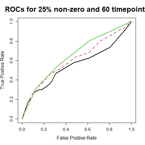
We also investigate how well the partial correlation graph is estimated under different methods when the samples are dependent, arising from a VAR process. The true graph is given by the nonzero entries in the true precision . The estimated graph is obtained by thresholding the estimated precision at a given level For the present investigation we use , i.e. two different time series nodes are declared connected if the partial correlation between the two components exceeds 0.15 in the estimated precision matrix. Figure 1 shows the ROC curves for the three estimation methods for different settings; two different sample sizes and two different sparsity levels In every case the proposed method has better performance than GCGM and GGM, with the GCGM performing better than the GGM. The AUC values for the proposed method are all bigger than those for the GCGM and GGM.
| Time points | 15% Non-zero | 25% Non-zero | ||||
|---|---|---|---|---|---|---|
| Causal VAR | GCGM | GGM | Causal VAR | GCGM | GGM | |
| 40 | 7.01 | 6.30 | 21.87 | 8.95 | 14.92 | 17.83 |
| 60 | 5.37 | 6.46 | 34.33 | 7.18 | 10.68 | 34.10 |


5.2 Graph Structure in US GDP Components
For graph estimation, the simulation experiment illustrated the benefit of explicitly accounting for temporal dependence in the sample. Here we analyze the graphical association among components of the US GDP based on time series data on each of the components. The data are obtained from bea.gov, collected quarterly for the period 2010 to 2019 with a total of 40 time points. We chose this particular period to avoid large external shocks like the Great Recession and the COVID-19 pandemic. We study 14 components that are used in the computation of the aggregate GDP value. Specifically, we study associations between the following components: Durable Goods (Dura), Nondurable Goods (NonDur), Services (Serv), Structures (Strct), Equipment (Equip), Intellectual Property Products (IPP), Residential Products (Resid), Exports-Goods (Exp-G), Exports-Services (Exp-S), Imports-Goods (Imp-G), Imports-Services (Imp-S), National Defense (NatDef), Nondefense expenditure (NonDef), State and Local expenditures (St-Lo). The time series for the components are reported independently. However, several of these variables share implicit dependencies. We apply our proposed model to study these dependencies.
The graphical structure is established based on the partial correlation graph obtained from estimating the stationary precision matrix. Figure 2 illustrates the estimated graphical dependence based on the estimated partial correlations with an absolute value of more than 0.15. Thresholding the partial correlations at 0.15 to determine active edges leads to 18 connections, about a fifth of the total possible edges. The partial correlation threshold was varied to check the sensitivity of the estimated graph to the choice of the threshold over the values ranging from 0.05 to 0.5.

| Dura | Nondur | Serv | Strct | Equip | IPP | Resid | Exp-G | Exp-S | Imp-G | Imp-S | NatDef | NonDef | St-Lo | |
| Dura | * | * | ||||||||||||
| NonDur | * | |||||||||||||
| Serv | * | |||||||||||||
| Strct | * | * | ||||||||||||
| Equip | * | * | * | * | ||||||||||
| IPP | * | * | ||||||||||||
| Resid | * | * | * | * | * | |||||||||
| Exp-G | * | * | * | * | * | |||||||||
| Exp-S | * | * | * | * | * | |||||||||
| Imp-G | * | |||||||||||||
| Imp-S | * | * | * | |||||||||||
| NatDef | * | * | ||||||||||||
| NonDef | * | * | ||||||||||||
| St-Lo | * |
To infer the estimated network, we compute graph theoretic nodal attributes. Specifically, we consider 1) Betweenness centrality, 2) Node impact, 3) Degree, 4) Participation coefficient, 5) Efficiency, 6) Average shortest path length, 7) Shortest path eccentricity, and 8) Leverage. For completeness, we provide a short description of these attributes in Section X of the supplementary materials.
From the attributes for the 14 GDP components, equipment, residential products, and export/import goods and services show a high degree of betweenness and centrality. These nodes seem to be deep in the graph. A better picture would emerge if the GDP components are studied at a more granular level in terms of their subcomponents. We plan to investigate that in the future.
| Dura | Nondur | Serv | Strct | Equip | IPP | Resid | Exp-G | Exp-S | Imp-G | Imp-S | NatDef | NonDef | St-Lo | |
|---|---|---|---|---|---|---|---|---|---|---|---|---|---|---|
| Betweenness | 9.000 | 0.000 | 0.000 | 10.000 | 39.000 | 10.000 | 34.000 | 50.000 | 34.000 | 0.000 | 14.000 | 2.000 | 5.000 | 0.000 |
| Node impact | 0.027 | -0.101 | -0.062 | 0.066 | -0.104 | 0.040 | -0.201 | -0.577 | 0.425 | -0.101 | 0.168 | -0.075 | -0.024 | -0.101 |
| Degree | 2.000 | 1.000 | 1.000 | 2.000 | 4.000 | 2.000 | 5.000 | 5.000 | 5.000 | 1.000 | 3.000 | 2.000 | 2.000 | 1.000 |
| Participation coefficient | 0.500 | 1.000 | 1.000 | 1.000 | 0.375 | 0.500 | 0.440 | 0.440 | 0.440 | 1.000 | 0.556 | 1.000 | 1.000 | 1.000 |
| Efficiency | 0.000 | 0.000 | 0.000 | 0.000 | 0.000 | 0.000 | 0.100 | 0.000 | 0.100 | 0.000 | 0.333 | 0.000 | 0.000 | 0.000 |
| Avg shortest pathlen | 2.071 | 2.786 | 2.571 | 2.071 | 1.714 | 2.000 | 1.929 | 1.929 | 1.643 | 2.786 | 1.857 | 2.643 | 2.357 | 2.786 |
| Shortest path eccentricity | 3.000 | 5.000 | 4.000 | 3.000 | 3.000 | 3.000 | 4.000 | 4.000 | 3.000 | 5.000 | 3.000 | 5.000 | 4.000 | 5.000 |
| Leverage | -0.381 | -0.667 | -0.600 | -0.314 | 0.178 | -0.429 | 0.355 | 0.460 | 0.244 | -0.667 | -0.100 | -0.214 | -0.214 | -0.667 |
6 Discussion
In this article, we propose a new Bayesian method for estimating the stationary precision matrix of a high-dimensional VAR process under stability constraints and subsequently estimating the contemporaneous stationary graph for the components of the VAR process. The method has several natural advantages. The methodology introduces a parameterization that allows fast computation of the stationary likelihood of a reduced rank high-dimensional Gaussian VAR process, a popular high-dimensional time series model. The new parameterization introduced here gives a natural way to directly model the sparse stationary precision matrix of the high-dimensional VAR process, which is the quantity needed to construct contemporaneous stationary graphs for the VAR time series. Most estimation methods for high-dimensional VAR processes fail to impose causality (or even stationarity) on the solution, thereby making estimating stationary precision matrix less meaningful. The proposed methodology uses causality as a hard constraint so that any estimate of the VAR process is restricted to the causal VAR space. We also show the posterior consistency of our Bayesian estimation scheme when priors are defined through the proposed parameterization. The focus of the present article is on the estimation of the stationary precision matrix of a high-dimensional stationary VAR. Hence, the direct parameterization of the precision, independent from other parameters involved in the temporal dynamics, is critical. However, a similar scheme can provide a direct parameterization of the VAR autocovariance matrices and, hence, the VAR coefficients under reduced rank and causality constraints for a high-dimensional VAR. This is part of future investigation. We also plan to investigate graph consistency for the partial correlation graph obtained by thresholding the entries of the stationary precision matrix of a high-dimensional VAR.
Funding
The authors would like to thank the National Science Foundation collaborative research grants DMS-2210280 (Subhashis Ghosal) / 2210281 (Anindya Roy) / 2210282 (Arkaprava Roy).
References
- Basu et al. [2015] S. Basu, A. Shojaie, and G. Michailidis. Network granger causality with inherent grouping structure. The Journal of Machine Learning Research, 16(1):417–453, 2015.
- Basu and Rao [2023] Sumanta Basu and Suhasini Subba Rao. Graphical models for nonstationary time series. The Annals of Statistics, 51:1453–1483, 2023.
- Bhattacharya and Dunson [2011] Anirban Bhattacharya and David B Dunson. Sparse Bayesian infinite factor models. Biometrika, 98(2):291–306, 2011.
- Chhikara [1988] Raj Chhikara. The Inverse Gaussian Distribution: Theory, Methodology, and Applications, volume 95. CRC Press, 1988.
- Christensen [2018] Alexander P Christensen. NetworkToolbox: Methods and measures for brain, cognitive, and psychometric network analysis in R. The R Journal, pages 422–439, 2018. doi: 10.32614/RJ-2018-065.
- Csárdi et al. [2024] Gábor Csárdi, Tamás Nepusz, Vincent Traag, Szabolcs Horvát, Fabio Zanini, Daniel Noom, and Kirill Müller. igraph: Network Analysis and Visualization in R, 2024. URL https://CRAN.R-project.org/package=igraph. R package version 2.0.3.
- Dahlhaus [2000] R. Dahlhaus. Graphical interaction models for multivariate time series. Metrika, 51:157––172, 2000.
- Fiecas et al. [2019] M. Fiecas, C. Leng, W. Liu, and Y Yu. Spectral analysis of high-dimensional time series. Electronic Journal of Statistics, 13(2):4079–4101, 2019.
- Friedman et al. [2008] Jerome Friedman, Trevor Hastie, and Robert Tibshirani. Sparse inverse covariance estimation with the graphical lasso. Biostatistics, 9(3):432–441, 2008.
- Ghosal and Van Der Vaart [2007] Subhashis Ghosal and Aad Van Der Vaart. Convergence rates of posterior distributions for noniid observations. The Annals of Statistics, 35(1):192–223, 2007.
- Ghosal and van der Vaart [2017] Subhashis Ghosal and Aad van der Vaart. Fundamentals of Nonparametric Bayesian Inference, volume 44 of Cambridge Series in Statistical and Probabilistic Mathematics. Cambridge University Press, Cambridge, 2017. ISBN 978-0-521-87826-5. doi: 10.1017/9781139029834. URL https://doi-org.prox.lib.ncsu.edu/10.1017/9781139029834.
- Ghosh et al. [2019] Satyajit Ghosh, Kshitij Khare, and George Michailidis. High-dimensional posterior consistency in bayesian vector autoregressive models. Journal of the American Statistical Association, 114(526):735–748, 2019.
- Haario et al. [2001] Heikki Haario, Eero Saksman, and Johanna Tamminen. An adaptive Metropolis algorithm. Bernoulli, 7(2):223–242, 2001.
- Heaps [2023] Sarah E Heaps. Enforcing stationarity through the prior in vector autoregressions. Journal of Computational and Graphical Statistics, 32(1):74–83, 2023.
- Jeong and Ghosal [2021] Seonghyun Jeong and Subhashis Ghosal. Unified bayesian theory of sparse linear regression with nuisance parameters. Electronic Journal of Statistics, 15(1):3040–3111, 2021.
- Joyce et al. [2010] Karen E Joyce, Paul J Laurienti, Jonathan H Burdette, and Satoru Hayasaka. A new measure of centrality for brain networks. PloS one, 5:e12200, 2010.
- Jung et al. [2015] A. Jung, G. Hannak, and N. Goertz. Graphical lasso based model selection for time series. IEEE Signal Processing Letters, 22(10):1781–1785, 2015.
- Kenett et al. [2011] Yoed N Kenett, Dror Y Kenett, Eshel Ben-Jacob, and Miriam Faust. Global and local features of semantic networks: Evidence from the hebrew mental lexicon. PloS one, 6:e23912, 2011.
- Koller and Friedman [2009] Daphne Koller and Nir Friedman. Probabilistic Graphical Models - Principles and Techniques. MIT Press, 2009.
- Lauritzen [1996] Steffen L. Lauritzen. Graphical Models. Oxford, 1996.
- Lütkepohl [2005] Helmut Lütkepohl. New Introduction to Multiple Time Series Analysis. Springer Science & Business Media, 2005.
- Ma and Michailidis [2016] Jing Ma and George Michailidis. Joint structural estimation of multiple graphical models. The Journal of Machine Learning Research, 17:5777–5824, 2016.
- Maathuis et al. [2019] Marloes Maathuis, Mathias Drton, Steffen L. Lauritzen, and Martin Wainwright, editors. Handbook of Graphical Models. Handbooks of Modern Statistical Methods. CRC Press, 2019.
- Ning et al. [2020] Bo Ning, Seonghyun Jeong, and Subhashis Ghosal. Bayesian linear regression for multivariate responses under group sparsity. Bernoulli, 26(3):2353–2382, 2020.
- Pons and Latapy [2005] Pascal Pons and Matthieu Latapy. Computing communities in large networks using random walks. In International symposium on computer and information sciences, pages 284–293. Springer, 2005.
- Qiu et al. [2016] Huitong Qiu, Fang Han, Han Liu, and Brian Caffo. Joint estimation of multiple graphical models from high dimensional time series. Journal of the Royal Statistical Society Series B: Statistical Methodology, 78(2):487–504, 2016.
- Roy et al. [2019] Anindya Roy, Tucker S Mcelroy, and Peter Linton. Constrained estimation of causal invertible varma. Statistica Sinica, 29(1):455–478, 2019.
- Roy et al. [2024] Arkaprava Roy, Anindya Roy, and Subhashis Ghosal. Bayesian inference for high-dimensional time series by latent process modeling. arXiv preprint arXiv:2403.04915, 2024.
- Shi et al. [2021] Wenli Shi, Subhashis Ghosal, and Ryan Martin. Bayesian estimation of sparse precision matrices in the presence of gaussian measurement error. Electronic Journal of Statistics, 15(2):4545–4579, 2021.
- Watson [2020] Christopher G. Watson. brainGraph: Graph Theory Analysis of Brain MRI Data, 2020. R package version 3.0.0.
- Zhang and Wu [2017] D. Zhang and W. B. Wu. Gaussian approximation for high dimensional time series. The Annals of Statistics, 45:1895–1919, 2017.
Supplementary materials
S1 Proof of the Main Theorems
We follow arguments in the general posterior contraction rate result from Theorem 8.19 of Ghosal and van der Vaart [2017] on the joint density of the entire multivariate time series by directly constructing a likelihood ratio test satisfying a condition like (8.17) of Ghosal and van der Vaart [2017]. We also use the simplified prior concentration condition (8.22) and global entropy condition (8.23) of Ghosal and van der Vaart [2017]. It is more convenient to give direct arguments than to fit within the notations of the theorem.
A.1 Prior concentration: pre-rate
Recall that the true parameter is denoted by , and the corresponding dispersion matrix is . We shall obtain the pre-rate satisfying the relation
| (A.1) |
where and , respectively, stand for the Kullback-Leibler divergence and Kullback-Leibler variation. To proceed, we show that the above event contains for some and estimate the probability of the latter, when is small.
We note that by Relation (iii) of Lemma 5, , while by Relation (i), , which are bounded by a constant by Condition (A5). Next observe that by Relation (iii) applied to , , where refers to the vector of the reciprocals of the entries of . Since the entries of lie between two fixed positive numbers, so do the entries of and when is small. Then it is immediate that (see, e.g., Lemma 4 of Roy et al. [2024]) that . Applying Lemma 8, we obtain the relation , which is small for sufficiently small. Thus, is also small. Since the operator norm is weaker than the Frobenius norm, this implies all eigenvalues of are close to zero. Now, expanding the estimates in Parts (ii) and (iii) of Lemma 4 in a Taylor series, the Kullback-Leibler divergence and variation between and are bounded by a multiple of if is chosen to be . The prior probability of is, in view of the assumed a priori independence of all components of , bounded below by for some constant . Hence . Thus (A.1) for , that is for , or any larger sequence.
A.2 Test construction
Recall that the true parameter is denoted by , and the corresponding dispersion matrix is . Let be another point in the parameter space such that the corresponding dispersion matrix satisfies , where is a large constant multiple of the pre-rate obtained in Subsection A.1. We first obtain a bound for the type I and type II error probabilities for testing the hypothesis against .
Let stand for the likelihood ratio test. Then, by the Markov inequality applied to the square root of the likelihood ratio, both error probabilities are bounded by , where stands for the Reyni divergence .
Let stand for the eigenvalues of . By Lemma 4, the Reyni divergence is given by . By arguing as in the proof of Lemma 1 of Roy et al. [2024], each term inside the sum can be bounded below by for some constants , where can be chosen as large as we like at the expense of making appropriately smaller. Under Condition (A4), using Relation (iii) of Lemma 5, we obtain that the are bounded by some constant not changing with . Thus, with a sufficiently large , the minimum operation in the estimate is redundant; that is, the Reyni divergence is bounded below by for some constant . This follows since and by Relation (iii) of Lemma 5, , which is bounded by a constant by Condition (A5). Thus both error probabilities are bounded by for some .
Now let be another parameter with the associated dispersion matrix such that , where is to be chosen sufficiently small. Then, using the Cauchy-Schwarz inequality and Part (iv) of Lemma 4, the probability of type II error of at is bounded by
| (A.2) |
Consider a sieve consisting of all alternative parameter points such that and , , for some constant to be chosen later, where is as in Condition (A2). By Part (i) of Lemma 5, for ,
which is bounded by for some constant as is fixed and . Thus the expression in (A.2) is bounded by for some constant by choosing a sufficiently small constant multiple of and large enough.
We have, 1) , 2) , and 3) .
Using 1), 2) and 3) above, we have i) ii) and iii) implies . Using the result from the above display, we let as Thus, at with , .
A.3 Rest of the proof of Theorem 2
To show that the posterior probability of converges to zero in probability, it remains to show that the prior probability of the complement of the sieve is exponentially small: for some sufficiently large .
Observe that
Since , the above expression is bounded by for some and can be chosen as large as we please by making in the definition of the sieve large enough. Hence, by arguing as in the proof of Theorem 8.19 of Ghosal and van der Vaart [2017], it follows that the posterior contraction rate for at in terms of the Frobenius distance is .
Let the collection of such with be denoted by , where . The number of such sets needed to cover is at most following the similar lines of arguments as in Lemma 8 of Roy et al. [2024] setting a negative polynomial in . Therefore . For each containing a point such that , we choose a representative and construct the likelihood ratio test . The final test for testing the hypothesis against the alternative is the maximum of these tests. Then, the resulting test has the probability of type II error bounded by while the probability of type I error is bounded by if we choose sufficiently large.
Finally, we convert the notion of convergence to those for and . Recall that the eigenvalues of are bounded between two fixed positive numbers, because by Lemma 5, and and and are assumed to have eigenvalues bounded between two fixed positive numbers. Now, applying Lemmas 6 and 7 respectively, and for all , for some constant . These relations yield the rate for the precision matrix and all regression coefficients at their respective true values in terms the Frobenius distance.
A.4 Proof of Theorem 3
When is sparse and the prior for imposes sparsity as described in Section 3.4, we show the improved rate . To this end, we refine the estimate of the prior concentration in Subsection A.1. The arguments used for the test construction, bounding the prior probability of the complement of the sieve and for converting the rate result in terms of the Frobenius distance on and remain the same. Except to control the number of nonzero entries in , we add in the sieve and let . Covering number calculation will remain identical to Lemma 8 of Roy et al. [2024].
Since is assumed to be a fixed constant, , , and so is the corresponding estimate for . For , the corresponding estimate does not change from the previous scenario. However, is now -dimensional instead of . The estimate for under the shrinkage prior improves to a multiple of by the arguments given in the proof of Theorem 4.2 of Shi et al. [2021]. Thus , leading to the asserted pre-rate . We also note that the additional sparsity imposed on through the prior does not further improve the rate when is a fixed constant and it may be replaced by a fully non-singular prior.
S2 Auxiliary lemmas and proofs
The following lemma expresses certain divergence measures in the family of centered multivariate normal distributions. The proofs follow from direct calculations.
Lemma 4.
Let and be probability densities of -dimensional normal distributions with mean zero and dispersion matrices and respectively. Let with eigenvalues . Then the following assertions hold:
-
(i)
The Reyni divergence is given by
-
(ii)
The Kullback-Leibler divergence is given by
-
(iii)
The Kullback-Leibler variation is given by
-
(iv)
If is positive definite, then expected squared-likelihood ratio is given by
which is bounded by
Lemma 5.
For all , we have
-
(i)
,
-
(ii)
,
-
(iii)
,
-
(iv)
,
-
(v)
Lemma 6.
We have is small if is small.
Lemma 7.
If is small, is small, where is the autoregressive coefficient.
The following Lemma is for around the truth case.
Lemma 8.
With , we have
assuming fixed lower and upper bounds on eigenvalues of and an upper bound for eigenvalues of .
Lemma 9.
With , and and for , Setting , and , we have,
where and .
The proof is based on next 5 Lemmas and results.
Lemma 10.
We have
Result 11 (Auxiliary recurrences).
We have,
-
1.
-
2.
-
3.
-
4.
Lemma 12 (Bounding first term of Lemma 10).
The bounds in terms of ’s,
| (A.1) | |||
| where | |||
| (A.2) |
where , for
Lemma 13 (Bounding second term of Lemma 10).
The final bounds for autoregressive coefficients,
| (A.3) |
where , .
The following steps will transform the bounds for ’s and ’s to ’s and ’s.
Lemma 14.
A.1 Proofs of the Auxiliary Lemmas and Resutls
Proof of Lemma 5.
Since,
The operator norm of is 1 and .
by applying the first inequality recursively as .
Applying the above, we also have,
The operator norm of is 1.
by applying the first inequality recursively as , .
Thus,
.
Since, , we have
∎
Proof of Lemma 6.
There are many diagonal blocks of and in and , respectively. Thus
and
. Thus, for small .
Hence, . This completes the proof.
∎
Proof of Lemma 7.
.
There are a total of blocks of in . Thus We have . Furthermore, .
In , there are diagonal blocks of ’s assuming divides , and thus . Hence, .
For not dividing is redundant in an asymptotic regime. ∎
Proof of Lemma 8.
We assume . Since, and , we have , and , we have,
And,
Finally,
| (A.4) |
where and .
While bounding around the truth, we let the eigenvalues of be bounded between two fixed constants. Also let be bounded by again a fixed constant. This puts an upper bound on as well. We have .
We can similarly show that,
We have, using the recurrence relations, that .
Then, we have if and . The constants will depend on the bounds on the truth.
∎
Proof of Lemma 9.
In the sieve, we have for some , a polynomial in .
We can similarly show that, for some which is polynomial in .
Then, we have if . In summary, we need , for some polynomial in , within for the above to hold.
Finally, for some which is polynomial in and the bound for is established above.
Thus, for some which is polynomial in
Within , if are all polynomials in , we have and which are also some polynomials in .
Setting, , we have , where .
Then using (A.4), we have the final result.
∎
Proof of Lemma 10.
We first compute a bound for VAR(1) case. Then use it for VAR(p).
From Lütkepohl [2005], we get for a VAR(1) process, where .
Using the telescopic sum setting , we have under our parametrization. Hence, .
and . We have and . Alternatively, .
Since, , we have . Hence
. Recursively using this relation and applying norm, we have , using the triangle inequality and the submultiplicative property of operator norm.
After some simplification using GP-series sum results, .
Hence,
.
.
.
And,
| (A.5) | |||
| (A.6) |
where and . Since, , we have . This comes in terms of the model parameters.
It is easy to verify that and are increasing in and, respectively. Following are the limits,
Proof of Result 11.
with .
.
We have and , .
We will be able to use mathematical induction to show that the difference can be bounded by the parameters.
Thus,
.
.
since .
Setting , we have since
Since, and
∎
S3 Attributes of the realized graph
The nodal attributes are computed using NetworkToolbox [Christensen, 2018], and brainGraph [Watson, 2020] in R. For the convenience of the reader, we briefly describe the definitions and characteristics of the nodal attributes. For a graph with nodes, let us denote the adjacency matrix by . Then, the degree of node is . The degree refers to the strength of each node in a graph. Global efficiency of the graph is measured by , where the shortest path length between the nodes and . The nodal efficiency is defined by , where is the subgraph of neighbors of and stands for the number of nodes in . The corresponding betweenness centrality is , where stands for the total number of the shortest paths from node to node and denotes the number of those paths that pass through . Nodal impact quantifies the impact of each node by measuring the change in average distances in the network upon removal of that node [Kenett et al., 2011]. The local shortest path length of each node is defined by the average shortest path length from that node to other nodes in the network. It is used to quantify the mean separation of a node in a network. Eccentricity is the maximal shortest path length between a node and any other node. Thus, it captures how far a node is from its most distant node in the network. Participant coefficient requires detecting communities first within the network. While using the R function participation of R package NetworkToolbox, we use the walktrap algorithm [Pons and Latapy, 2005] to detect communities. The participation coefficient quantifies the distribution of a node’s edges among different communities in the graph. It is zero if all the edges of a node are entirely restricted to its community, and it reaches its maximum value of 1 when the node’s edges are evenly distributed among all the communities. Within-community centrality is used to describe how central a node’s community is within the whole network. We use the walktrap algorithm to detect the communities. The final centrality measure that we include in our study is leverage centrality, introduced by Joyce et al. [2010]. Leverage centrality is the ratio of the degree of a node to its neighbors, and it thus measures the reliance of its immediate neighbors on that node for information.