Bath’s law, correlations and magnitude distributions

Bath’s law states that the average difference $\Delta M$ between the magnitude of a main shock and the magnitude of its largest aftershock is independent of the magnitude of the main shock (Bath, 1965; see also Richter, 1958). The reference value of the average magnitude difference is $\Delta M=1.2$. Deviations from this value have been reported (see, for instance, Lombardi, 2002; Felzer et al, 2002; Console et al, 2003), some being discussed by Bath, 1965.

The Bath’s law is an empirical statistical law. The earliest advance in understanding its origin was made by Vere-Jones, 1969, who viewed the main shock and its aftershocks as statistical events of the same statistical ensemble, distributed in magnitude. The magnitude-difference distribution introduced by Vere-Jones, 1969, may include correlations, which are viewed sometimes as indicating the opinion that the main shocks are statistically distinct from the aftershocks, or the foreshocks (Utsu, 1969, Evison and Rhoades, 2001). The Bath’s law enjoyed many discussions and attempts of elucidation (Papazachos, 1974; Purcaru, 1974; Tsapanos, 1990; Kisslinger and Jones, 1991; Evison, 1999; Lavenda and Cipollone, 2000; Lombardi, 2002; Helmstetter and Sornette, 2003). The prevailing opinion ascribes the variations in $\Delta M$ to the bias in selecting data and the insufficiency of the realizations of the statistical ensemble. This standpoint was substantiated by means of the binomial distribution (Console, 2003; Lombardi, 2002; Helmstetter and Sornette, 2003). In order to account for the deviations of $\Delta M$ Helmstetter and Sornette, 2003, employed the ETAS (epidemic-type aftershock sequence) model for the differences in the selection procedure of the mainshocks and the aftershocks. According to this model the variations in the number $\Delta M$ are related to the realizations of the statistical ensemble and the values of the fitting parameters (see also Lombardi, 2002; Console, 2003).

The statistical hypothesis for the distributions of earthquake time series is far-reaching. Usually, a statistical distribution is (quasi-) independent of time (it is an equilibrium distribution), such that the aftershocks, distributed in the "future", should be identical with the foreshocks, distributed in the "past". However, it seems that there are differences between these two empirical distributions (Utsu, 2002; Shearer, 2012). Moreover, in order the statistical laws to be operational in practice, we need to have a large statistical ensemble of accompanying (associated) earthquakes, identified as aftershocks and foreshocks, which is a difficult issue in empirical studies. In addition, the empirical realizations of the statistical ensembles of earthquakes should be repetitive, a point which raises problems of principle, considering the variations in time and locations. In order to get meaningful results by applying the statistical laws to physical ensembles, it is necessary to prepare, in the same conditions, identical realizations of such ensembles. This is possible in Statistical Physics for various physical systems (like gases, liquids, solids,. etc). However, an ensemble of earthquakes, collected from a given zone in a (long) period of time, is not reproducible, because the conditions of its realization cannot be reproduced: the distribution of the focal regions may change in the given zone, or in the next period of time, including the change in physical (geological) conditions. The application of the statistical method to earthquakes exhibits limitations.

We show in this paper that the appropriate tool of approaching the accompanying seismic activity (foreshocks and aftershocks) of the main shocks is the distribution function of the difference in magnitude. The derivation of this distribution is made herein by means of the conditional probabilities (the Bayes theorem), as well as by using pair distributions. The earthquake correlations can be expressed by means of the magnitude-difference distribution. These correlations may be dynamical, or purely statistical. The dynamical correlations arise from an "earthquake interaction", while the purely statistical correlations originate in other, unknown, causes. Pair distributions related to statistical correlations are presented. The singe-event distribution of dynamically correlated earthquakes is derived from the statistical fluctuations of the accumulation time, by means of the geometric-growth model of energy accumulation in the focal region. The dynamical correlations may account, at least partially, for the roll-off effect in the Gutenberg-Richter statistical distributions. The difference in magnitude is extended to negative values, leading to a symmetric distribution for the foreshocks and aftershocks, with a vanishing mean value for the magnitude difference. This suggests to view the accompanying seismic activity as representing fluctuations, and to take their standard deviation as a measure for the Bath’s average difference $\Delta M$ between the magnitude of the main shock and its largest aftershock (foreshock). This way, the Bath’s law is deduced. It is shown that moderate-magnitude doublets may be viewed as "Bath partners". Deterministic time-magnitude correlations of the associated seismic activity are also presented.

According to the geometric-growth model of energy accumulation in a localized focal region (Apostol, 2006a,b), the accumulated energy $E$ is related to the accumulation time $t$ by

$$1+t/t_{0}=\left(1+E/E_{0}\right)^{r}\,\,\,,$$

(1)

where $t_{0}$ and $E_{0}$ are time and energy thresholds and $r$ is a geometrical parameter which characterizes the focal region. This parameter is related to the reciprocal of the number of effective dimensions of the focal region and to the strain accumulation rate (which, in general, is anisotropic). Very likely, the parameter $r$ varies in the range $1/3<r<1$. For a pointlike focal region with a uniform accumulation rate $r=1/3$ (three dimensions), for a two-dimensional uniform focal region $r=1/2$, while for a one-dimensional focal region $r$ tends to unity. An average parameter $r$ may take any value in this range.

In equation (1) the threshold parameters should be viewed as very small, such that $t/t_{0},\,E/E_{0}\gg 1$ and equation (1) may be written as

$$t/t_{0}\simeq\left(E/E_{0}\right)^{r}\,\,.$$

(2)

A uniform frequency of events $\sim t_{0}/t$ in time $t$ indicates that the parameter $t_{0}$ is the reciprocal of the seismicity rate $1/t_{0}$. It follows immediately the time distribution

$$P(t)dt=\frac{1}{\left(t/t_{0}\right)^{2}}\frac{dt}{t_{0}}$$

(3)

and, making use of equation (2), the energy distribution

$$P(E)dE=\frac{r}{\left(E/E_{0}\right)^{1+r}}\frac{dE}{E_{0}}\,\,.$$

(4)

At this point we may use an exponential law $E/E_{0}=e^{bM}$, where $M$ is the earthquake magnitude and $b=\frac{3}{2}\cdot\ln 10=3.45$, according to Kanamori, 1977, and Hanks and Kanamori, 1979 (see also, Gutenberg and Richter, 1944, 1956); we get the (normalized) magnitude distribution

$$P(M)dM=\beta e^{-\beta M}dM\,\,\,,$$

(5)

where $\beta=br$. In decimal logarithms, $P(M)=(1.5r)\cdot 10^{-(1.5r)M}$, where $0.5<1.5r<1.5$ (for $1/3<r<1$). Usually, the average value $1.5r=1$ ($\beta=2.3$) is currently used as a reference value, corresponding to $r=2/3$ (see, for instance, Stein and Wysesssion, 2003; Udias, 1999; Lay and Wallace, 1995; Frohlich and Davis, 1993). Since $t\gg t_{0}$, $E\gg E_{0}$, the magnitude distribution given by equation (5) is not adequate for very small magnitudes ($M\longrightarrow 0$).

It is worth noting that the magnitude distribution (equation (5)) has the property $P(M_{1}+M_{2})\sim P(M_{1})P(M_{2})$, while the time and energy distributions (equations (3) and (4)) have not this property. This is viewed sometimes as indicating that the earthquakes would be correlated in occurrence time and in energy (Corral, 2006).

The magnitude distribution is particularly important because it can be used to analyze the empirical distribution

$$P(M)=\frac{\Delta N}{N_{0}\Delta M}=\frac{t_{0}\Delta N}{T\Delta M}\,\,\,,$$

(6)

of $\Delta N$ earthquakes with magnitude in the range $(M,\,M+\Delta M)$ out of a total number $N_{0}=T/t_{0}$ of earthquakes which occurred in time $T$. We get

$$\ln\left(\Delta N/T\right)=\ln\left(\frac{\beta\Delta M}{t_{0}}\right)-\beta M\,\,.$$

(7)

From the magnitude frequency $\Delta N/T$ (equation (6)) we get the mean recurrence time

$$t_{r}=\frac{t_{0}}{\beta\Delta M}e^{\beta M}$$

(8)

for an earthquake with magnitude $M$ (i.e. in the interval $(M,\,M+\Delta M)$). This time should be compared with the accumulation time $t_{a}=t_{0}e^{\beta M}$ for an earthquake with magnitude $M$, given by equation (2) and the exponential law $E/E_{0}=e^{bM}$. These times are related by $t_{a}=(\beta\Delta M)t_{r}$, whence one can see that $t_{a}<t_{r}$ (for $\beta\Delta M<1$), a relationship which shows that the energy corresponding to a magnitude $M$ may be lost by seismic events lower in magnitude, as expected. Moreover, by the definition of the seismicity rate, an earthquake with magnitude $M$ is equivalent with a total number $t_{a}/t_{0}=e^{\beta M}$ of earthquakes with zero magnitude (energy $E_{0}$) (Michael and Jones, 1998; Felzer et al, 2002). We may call these earthquakes (defined by the seismicity rate) "fundamental earthquakes" corresponding to magnitude $M$. It is worth noting that the magnitude distribution $\beta e^{-\beta M}$ implies an error of the order $\left(\sqrt{\overline{M^{2}}}-\overline{M}\right)/\overline{M}=\sqrt{2}-1$, at least, i.e., $\Delta t_{r}/t_{r}\simeq 0.41$. For a maximal entropy with mean recurrence time $t_{r}$ we get easily a Poisson distribution $(1/t_{r})e^{-t/t_{r}}$ for the recurrence time, which has a (large) standard deviation $\sqrt{\overline{(t-t_{r})^{2}}}=t_{r}$.

Similarly, from equation (5) we get the excedence rate (the so-called recurrence law), which gives the number $N_{ex}$ of earthquakes with magnitude greater than $M$. The corresponding probability is readily obtained from (5) as $P_{ex}=e^{-\beta M}$, such that the excedence rate reads

$$\ln N_{ex}=\ln N_{0}-\beta M\,\,.$$

(9)

The distributions given above may be called Gutenberg-Richter statistical distributions (equations (7) and (9) and, implicitly, (5)). They are currently used in statistical analysis of the earthquakes. The parameter $\beta$ is derived by fitting these distributions to data. For $1/3<r<1$ it varies in the range $1.15<\beta<3.45$ (for decimal logarithms $0.5<1.5r<1.5$). For instance, an analysis of a large set of global earthquakes with $5.8<M<7.3$ ($\Delta M=0.1$) indicates $\beta=1.38$ (and $1/t_{0}=10^{5.5}$ per year), corresponding to $r=0.4$, a value which suggests an intermediate two/three-dimensional focal mechanism (Bullen, 1963). For $r=1/3$, corresponding to a uniform pointlike focal geometry, we get $\beta=1.15$. Equations (5), (7) and (9) have been fitted to a set of $1999$ earthquakes with magnitude $M\geq 3$ ($\Delta M=0.1$), which occurred in Vrancea between $1974-2004$ ($31$ years) (Apostol 2006a,b). The mean values of the fitting parameters are $-\ln t_{0}=9.68$ and $\beta=1.89$ ($r=0.54$). A similar fit has been done for a set of $3640$ earthquakes with magnitude $M\geq 3$ which occurred in Vrancea during $1981-2018$ ($38$ years). The fitting parameters for this set are $-\ln t_{0}=11.32$ and $\beta=2.26$ ($r=0.65$). The data for Vrancea have been taken from the Romanian Earthquake Catalog, 2018. The parameter $\beta$ varies from region to region, depends on the nature of the focal mechanism (parameter $r$ in $\beta=br$), the size and the time period of the data set. The range of empirical values $0.5<1.5r<1.5$ coincides with the theoretical range ($1/3<r<1$).

The statistical analysis gives a generic image of a collective, global earthquake focal region (a distribution of foci). Particularly interesting is the parameter $r$, which is related to the reciprocal of the (average) number of effective dimensions of the focal region and the rate of energy accumulation. The value $r=0.54$ (Vrancea, period $1974-2004$) indicates a (quasi-) two-dimensional geometry of the focal region in Vrancea, while the more recent value $r=0.65$ for the same region suggests an evolution of this (average) geometry towards one dimension. At the same time, we note an increase of the seismicity rate $1/t_{0}$ in the recent period in Vrancea. The increase of the geometrical parameter $r$ determines an increase of the parameter $\beta$, which dominates the mean recurrence time. For instance, the accumulation time for magnitude $M=7$ is increased from $t_{a}\simeq 34.9$ years (period $1974-2004)$ to at least $t_{a}\simeq 59$ years. This large variability indicates the great sensitivity of the statistical analysis to the data set. In particular, for any fixed $M$ we may view the exponential $Me^{-M\beta}$ as a distribution of the parameter $\beta$, which indicates an error $\simeq 0.41$ in determining this parameter.

We note that inherent errors occur in statistical analysis. For instance, an error is associated to the threshold magnitude (e.g., $M=3$), because the large amount of data with small magnitude may affect the fit. Also, it is difficult to include events with high magnitude in a set with statistical significance, because such events are rare. The size of the statistical set may affect the results. The fitting values given above for Vrancea have an error of approximately $15\%$. Such difficulties are carefully analyzed on various occasions (e.g., Felzer et al, 2002; Console et al, 2003; Lombardi, 2002; Helmstetter and Sornette, 2003).

The statistical distributions given above may be employed to estimate conditional probabilities, and to derive Omori laws for the associated (accompanying) seismic activity. Also, the conditional probabilities can be used for analyzing the next-earthquake distributions (inter-event time distributions), (Apostol and Cune, 2020) which may offer information for seismic hazard and risk estimation. We present here another example of using these distributions, in analyzing the Bath’s empirical law.

In general, two or more earthquakes may appear as being associated in time and space with, or without, a mutual interaction between their focal regions. In both cases they form a foreshock-main shock-aftershock sequence which exhibits correlations. The correlations which appear as a consequence of an interaction imply an energy transfer (exchange) between the focal regions (e.g., a static stress). These correlations may be called dynamical (or "causal") correlations. Another type of correlations may appear without this interaction, from unknown causes. For instance, an earthquake may produce changes in the neighbourhood of its focal region (adjacent regions), and these changes may influence the occurrence of another earthquake. Similarly, an associated seismic activity may be triggered by a "dynamic stress", not a static one (Felzer and Brodsky, 2006). "Unknown causes" is used here in the sense that the model employed for describing these earthquakes does not account for such causes. The correlations arising from "unknown causes" may be called purely statistical (or "acausal") correlations. It is worth noting that all the correlations discussed here have a statistical character.

Let us first discuss the dynamical correlations. If an amount $\delta E$ of energy (positive or negative) is provided to a focal region by neighbouring focal regions, the accumulation time $t$ in the time-energy accumulation law $t/t_{0}=(E/E_{0})^{r}$ (equation (2)) changes. For a given energy we may assign this variation to the parameter $r$. This may correspond to a change in the focal region subject to interaction (as, for instance, one produced by a static stress). We are led to examine the changes in the accumulation time $t$. We have shown above that the ratio $t/t_{0}$ is the number $n_{0}=e^{\beta M}$ of "fundamental earthquakes" corresponding to the magnitude $M$, where $t_{0}$ is the cutoff time (time threshold; equations (2) to (5)). We may write, approximately, this (large) number as the sum

$$n_{0}=\sum_{i=1}^{n_{0}}n_{i}\,\,,\,\,n_{i}=1\,\,.$$

(10)

In this equation we may view $n_{i}$ as statistical variables, with mean value $\overline{n}_{i}=1$. Therefore, we consider the number of fundamental earthquakes

$$n=\sum_{i=1}^{n_{0}}n_{i}\,\,\,,$$

(11)

with the mean value $\overline{n}=n_{0}$. The variables $n_{i}$ are viewed as independent statistical variables; their fluctuations are due to the interaction of these fundamental earthquakes with other fundamental earthquakes, corresponding to different magnitudes (exchange of numbers of fundamental earthquakes). These interactions play the role of an external "thermal bath" for the fundamental earthquakes corresponding to a given magnitude $M$. Therefore, the deviation $\Delta n=\sqrt{\overline{(\delta n)^{2}}}$ (where $\delta n=n-n_{0}$, $\delta n_{i}=n_{i}-\overline{n}_{i}$) is the number $n_{c}$ of (dynamically) correlated fundamental earthquakes corresponding to $M$. We get immediately

$$\overline{(\delta n)^{2}}=\sum_{i,j=1}^{n_{0}}\overline{\delta n_{i}\delta n_{j}}=\sum_{i=1}^{n_{0}}\overline{(\delta n_{i})^{2}}=a^{2}n_{0}\,\,\,,$$

(12)

where $a^{2}=\overline{(\delta n_{i})^{2}}$ (independent of $i$). It follows

$$n_{c}=a\sqrt{n_{0}}=ae^{\frac{1}{2}\beta M}\,\,.$$

(13)

Obviously, this number is $t_{c}/at_{0}$, where $t_{c}$ is the accumulation time for the correlated earthquakes with magnitude $M$ (in order to preserve the correspondence of the cutoff time and energy parameters we need to re-define the cutoff time $t_{0}$ as $at_{0}$). Now, we can repeat the derivation from equations (2) to (5) and get the magnitude probability of the correlated earthquakes

$$P_{c}(M)=\frac{1}{2}\beta e^{-\frac{1}{2}\beta M}\,\,.$$

(14)

We note that in the energy-accumulation law given by equation (2) the parameter $r$ changes to $r/2$ for dynamically correlated earthquakes ($t_{c}/at_{0}=(E/E_{0})^{r/2}$).

The dynamically correlated earthquakes may be present in foreshock-main shock-aftershock sequences. It is difficult to test empirically the probability $P_{c}(M)$, because we cannot see any means to separate the dynamical correlations from the purely statistical correlations. We note that the dynamically correlated earthquakes are distinct from the rest of the earthquakes (their distribution $\sim e^{-\frac{1}{2}\beta M}$ is different from the distribution $\sim e^{-\beta M}$). Usually, in empirical studies we do not make this difference (see, for instance, Kisslinger, 1996), but the error may be neglected, because the total number of earthquakes $N_{0}$ is much larger than the total number of dynamically correlated earthquakes $N_{c}$, according to equations (5), (6) and (14) ($N_{c}^{2}=(4\Delta N_{c}^{2}/\Delta N\Delta M)N_{0}$); $N_{c}$ is, simply, proportional to the statistical error $\sqrt{N_{0}}$. Like the total number of earthquakes, the dynamically correlated earthquakes are concentrated in the region of small magnitudes, where the slope of the function $\ln P_{c}(M)$ is changed from $-\beta$ to $-\frac{1}{2}\beta$. Such a deviation is well known in empirical studies (the roll-off effect; Pelletier, 2000; Bhattacharya et al, 2009), and is attributed usually to an insufficient determination of the small-magnitude data. Moreover, small-magnitude correlated earthquakes in foreshock-main shock-aftershock sequences are associated with high-magnitude main shocks, which have a large productivity of accompanying events. Therefore, dynamically correlated earthquakes are expected in earthquake clusters with high-magnitude main shocks.

The Bath’s law is expressed in terms of the difference in magnitude between the main shock and its largest aftershock. Let us first consider two earthquakes with magnitudes $M_{1,2}$, with the distribution law $\sim e^{-\beta M}$, $M=M_{1,2}$, and seek the distribution of the difference in magnitude $m=M_{1}-M_{2}$. In this law the magnitude $M$ is positive, but for the difference $M_{1}-M_{2}$ we need to extend this variable to negative values. Since $M_{1}=M_{1}-M_{2}+M_{2}$ and $M_{2}=M_{2}-M_{1}+M_{1}$, the law $\sim e^{-\frac{1}{2}\beta M}$ suggests a magnitude-difference distribution $\sim e^{-\beta(M_{1}-M_{2})}$ for $M_{1}>M_{2}$ and fixed $M_{2}$, and a distribution $\sim e^{-\beta(M_{2}-M_{1})}$ for $M_{2}>M_{1}$ and fixed $M_{1}$. These are conditional probabilities (related to the Bayes theorem). In both cases, this distribution can be written as $\sim e^{-\beta\mid m\mid}$, where $m=M_{1}-M_{2}$ (or $m=M_{2}-M_{1}$), $\mid m\mid<max(M_{1},M_{2})$, irrespective of which $M_{1,2}$ is fixed. The condition $\mid m\mid<max(M_{1},M_{2})$ is essential for statistical correlations. We pass now to the Bath’s law. Let us assume a main shock, with magnitude $M_{s}$, and the accompanying earthquakes (foreshocks and aftershocks), with magnitude $M$. We define the foreshocks and aftershocks as those correlated earthquakes with magnitude $M$ smaller than $M_{s}$. We refer the magnitudes $M$ of the foreshocks and aftershocks to the magnitude $M_{s}$ of the main shock, by observing the ordering of the partners in each pair. This can be done by defining $m=M_{s}-M>0$ for foreshocks and $m=M-M_{s}<0$ for aftershocks. According to the above discussion, the distribution of the magnitude difference is $\sim e^{-\beta\mid m\mid}$, $\mid m\mid<M_{s}$. Therefore, the total distribution is

$$P(M_{s},m)=\beta^{2}e^{-\beta M_{s}}e^{-\beta\mid m\mid}\,\,,\,\,\mid m\mid<M_{s}\,\,,\,\,M_{s}>0\,\,.$$

(15)

This is a pair distribution, for two events $M_{s}$ and $m$.

Let us apply first this law to dynamically-correlated earthquakes, by replacing $\beta$ in equation (15) by $\beta/2$. Since these earthquake clusters are associated with high-magnitude main shocks we may omit the condition $\mid m\mid<M_{s}$, and let $\mid m\mid$ go to infinity. In this case the statistical correlations are lost; we are left only with the dynamical correlations. The distribution given by equation (15) becomes a distribution of two independent events, identifed by $M_{s}$ and $m$; we may use only the magnitude difference distribution

$$p_{c}(m)=\frac{1}{4}\beta e^{-\frac{1}{2}\beta\mid m\mid}\,\,,\,\,-\infty<m<+\infty\,\,.$$

(16)

This distribution has a vansihing mean value $\overline{m}$ ($\overline{m}=0$). The next correction to this mean value, i.e. the smallest deviation of $m$, is the standard deviation

$$\Delta m=\sqrt{\overline{m^{2}}}=\frac{2\sqrt{2}}{\beta}\,\,.$$

(17)

Therefore, we may conclude that the average difference in magnitude between the main shock and its largest aftershock (or foreshock) is given by the standard deviation $\Delta M=\Delta m=2\sqrt{2}/\beta$. This is the Bath’s law. The number $2\sqrt{2}/\beta$ does not depend on the magnitude $M_{s}$ (but it depends on the parameter $\beta$, corresponding to various realizations of the statistical ensemble). It is worth noting that $\Delta m$ given by equation (17) implies an averaging (of the squared magnitude differences). Making use of the reference value $\beta=2.3$ we get $\Delta M=1.23$, which is the Bath’s reference value for the magnitude difference. In the geometric-growth model the reference value $\beta=2.3$ corresponds to the parameter $r=2/3$. We can check that higher-order moments $\overline{m^{2n}}$, $n=2,3,...$ are larger than $\overline{m^{2}}$ (for any value of $\beta$ in the range $1.15<\beta<3.45$).

The result $\Delta M=2\sqrt{2}/\beta$ could be tested empirically, although, as it is well known, there exist difficulties. In empirical studies the magnitude difference $\Delta M$ is variable, depending on the fitting parameter $\beta$, which can be obtained from the statistical analysis of the data. The results may tend to the value $\Delta M=1.2$ by adjusting the cutoff magnitudes (Lombardi, 2002; Console, 2003), or by choosing particular values of fitting parameters (Helmstetter and Sornette, 2003); there are cases when the data exhibit values close to $\Delta M=1.2$ (Felzer et al, 2002). It seems that values closer to $\Delta M=1.2$ occur more frequently in the small number of sequences which include high-magnitude main shocks.

If we extend the dynamical correlations to moderate-magnitude main shocks, we need to keep the condition $\mid m\mid<M_{s}$, such that the distribution is

$$P_{c}(M_{s},m)=\frac{1}{4}\beta^{2}e^{-\frac{1}{2}\beta M_{s}}e^{-\frac{1}{2}\beta\mid m\mid}\,\,,\,\,\mid m\mid<M_{s}\,\,,\,\,M_{s}>0\,\,.$$

(18)

The standard deviation is now $\Delta M=\Delta m=\sqrt{2}/\beta$, which leads to $\Delta M\simeq 0.61$ for the reference value $\beta=2.3$. Such a variablility of $\Delta M$ can often be found in empirical studies. For instance, from the analysis made by Lombardi, 2002, of Southern California earthquakes 1990-2001 we may infere $\beta\simeq 2$ and an average $\Delta M\simeq 0.45$ (with large errors). From Console et al, 2003, New Zealand catalog (1962-1999) and Preliminary Determination of Epicentres catalog (1973-2001), we may infere $\beta\simeq 2.5-2.3$ and an average $\Delta M=0.43-0.54$, respectively, while $\Delta M=\sqrt{2}/\beta$ gives $0.56-0.61$. In other cases, like the California-Nevada data analyzed by Felzer et al, 2002, the parameters are $\beta=2.3$ and $\Delta M\simeq 1.2$, in agreement with $\Delta M=2\sqrt{2}/\beta$. We note that $\Delta M=\sqrt{2}/\beta$ given here is an over-estimate, because it extends, in fact, the dynamical correlations (equation (14)) to small-magnitude main shocks.

Leaving aside the dynamical correlations we are left with purely statistical correlations for clusters with moderate-magnitude main shocks. In this case we use the distribution given by equation (15), which leads to $\Delta M=$$\Delta m=1/\sqrt{2}\beta$ and $\Delta M=0.31$ for the reference vale $\beta=2.3$. The Bath partner for such a small value of the magnitude difference looks rather as a doublet (Poupinet et al, 1984; Felzer et al, 2004).

For statistical correlations we can compute the correlation coefficient (variance). The correlation coefficient $R=\overline{M_{s}M}/\Delta M_{s}\Delta M$ between the main shock and an accompanying event $M=M_{s}-\mid m\mid$ ($\mid m\mid<M_{s}$) computed by using the distribution given in equation (15) is $R=2/\sqrt{5}$. For the correlation coefficient beteen two accompanying events $M_{1}$ and $M_{2}$ we need the three-events distribution (which includes $M_{1,2}$ and $M_{s}$).

In general, the correlations are visible in the pair (two-event, bivariate) distributions. Such distributions are obtained as the mixed second-order derivative of a generating function of two variables. We give here the pair distribution derived from the geometric-growth model of energy accumulation. We show that it coincides, practically, with the pair distribution used above (equation (15)). Moreover, the pair distribution derived here exhibits the dynamical correlations. The single-event probability $P(t)$ given by equation (3) is obtained as the derivative $P(t)=-\partial F/\partial t$ of the frequency function $F(t)=t_{0}/t$. Similarly, by using the change of variable $t/t_{0}=e^{\beta M}$, we get the Gutenberg-Richter magnitude distribution $P(M)=\beta e^{-\beta M}$ from $P(M)=-\partial F/\partial M$, where $F(M)=e^{-\beta M}$ (equation (5)).

Let us assume that two successive earthquakes may occur in time $t$, one after time $t_{1}=t_{0}e^{\beta M_{1}}$, another after time $t_{2}=t_{0}e^{\beta M_{2}}$ from the occurrence of the former. Using the partition $t=t_{1}+t_{2}$ we get the distribution

$$P(t_{1},t_{2})\sim\frac{\partial^{2}F}{\partial t_{1}\partial t_{2}}=\frac{2t_{0}}{(t_{1}+t_{2})^{3}}\,\,,$$

(19)

or, properly normalized,

$$P(M_{1},M_{2})=4\beta^{2}\frac{e^{\beta(M_{1}+M_{2})}}{\left(e^{\beta M_{1}}+e^{\beta M_{2}}\right)^{3}}\,\,.$$

(20)

We can see that this distribution is different from $P(M_{1})P(M_{2})=\beta^{2}e^{-\beta(M_{1}+M_{2})}$, which indicates that the two events $M_{1,2}$ are correlated.

Let $M_{1}=M_{2}+m$ and $M_{1}>M_{2}$, $0<m<M_{1}$; equation (20) becomes

$$P(M_{1},M_{2})=4\beta^{2}\frac{e^{-\beta M_{1}}e^{-\beta m}}{\left(1+e^{-\beta m}\right)^{3}}\,\,;$$

(21)

similarly, for $M_{2}>M_{1}$, $-M_{2}<m<0$ we get

$$P(M_{1},M_{2})=4\beta^{2}\frac{e^{-\beta M_{2}}e^{\beta m}}{\left(1+e^{\beta m}\right)^{3}}\,\,.$$

(22)

It follows that we may write

$$P(M_{1},M_{2})=4\beta^{2}\frac{e^{-\beta max(M_{1},M_{2})}e^{-\beta\mid m\mid}}{\left(1+e^{-\beta\mid m\mid}\right)^{3}}\,\,\,,$$

(23)

which highlights the magnitude-difference distribution, with the constraint $\mid m\mid<max(M_{1},M_{2})$.

Let $M_{s}$ and $M$ be the magnitudes of the main shock and an acompanying earthquake (foreshock or aftershock), respectively. We define the ordered magnitude difference $m=M_{s}-M>0$ for foreshocks and $m=M-M_{s}<0$ for aftershocks, $\mid m\mid<M_{s}$. According to equation (23), the distribution of the pair consisting of the main shock and an acompanying event is

$$P(M_{s},m)=4\beta^{2}e^{-\beta M_{s}}\frac{e^{-\beta\mid m\mid}}{\left(1+e^{-\beta\mid m\mid}\right)^{3}}\,\,,\,\,\mid m\mid<M_{s}.$$

(24)

The exponential $e^{-\beta\mid m\mid}$ falls off rapidly to zero for increasing $m$, so we may neglect it in the denominator in equation (24). We are left with the pair distribution given by equation (15) (properly normalized).

If we integrate equation (20) with respect to $M_{2}$ (and redefine $M_{1}=M$), we get the so-called marginal distribution

$$P_{mg}(M)=\beta e^{-\beta M}\frac{2}{\left(1+e^{-\beta M}\right)^{2}}\,\,.$$

(25)

This distribution differs appreciably from the Gutenberg-Richter distribution $\beta e^{-\beta M}$ for $\beta M$$\ll 1$ and only slightly (by an almost constant factor $\simeq 2$) for moderate and large magnitudes. The corresponding cummulative distribution for all magnitudes greater than $M$

$$P_{mg}^{ex}(M)=e^{-\beta M}\frac{2}{1+e^{-\beta M}}$$

(26)

can be written as

$$P_{mg}^{ex}(M)\simeq e^{-\beta M}\frac{1}{1-\frac{1}{2}\beta M}\simeq e^{-\frac{1}{2}\beta M}$$

(27)

in the limit $M\longrightarrow 0$, which indicates that the slope of the excedence rate $\ln P_{mg}^{ex}(M)$ deviates from $-\beta$, corresponding to the usual Gutenberg-Richter exponential distribution, to $-\frac{1}{2}\beta$ (the roll-off effect). This deviation indicates the presence of dynamical correlations governed by the distribution law $P_{c}(M)=\frac{1}{2}\beta e^{-\frac{1}{2}\beta M}$ (equation (14)).

The pair distribution given above can be written both for the earthquakes governed by the Gutenberg-Richter distribution $\sim e^{-\beta M}$ and for the sub-set of dynamically-correlated earthquakes governed by the distribution $\sim e^{-\frac{1}{2}\beta M}$. The procedure of extracting dynamically-correlated earthquakes can be iterated, passing from $\beta/2$ to $\beta/4$, etc; however, the number of affected earthquakes tends rapidly to zero, and the procedure becomes irrelevant.

We may assume that energy $E$ is released by two successive earthquakes with energies $E_{1,2}=E_{0}e^{bM_{1,2}}$, such that $E=E_{1}+E_{2}$. The time corresponding to the energy $E$ is $t=t_{0}\left(E_{1}/E_{0}+E_{2}/E_{0}\right)^{r}$, or $t=t_{0}\left(e^{bM_{1}}+e^{bM_{2}}\right)$. We cannot derive a pair distribution from the second-order derivative of $t_{0}/t=\left(e^{bM_{1}}+e^{bM_{2}}\right)^{-1}$, because the variation of the magnitudes $M_{1,2}$ implies the variation of the energies $E_{1,2}$, and not of the times $t_{1,2}$. This would contradict the geometric-growth model which assumes that the probabilities are given by time derivatives.

Let us assume that the amount of energy $E$ accumulated in time $t$ is released by two successive earthquakes with energies $E_{1,2}$, such as $E=E_{1}+E_{2}$. Since, according to equation (2),

$$\begin{array}[]{c}t/t_{0}=(E/E_{0})^{r}=\left(E_{1}/E_{0}+E_{2}/E_{0}\right)^{r}<\\ \\ <(E_{1}/E_{0})^{r}+(E_{2}/E_{0})^{r}=t_{1}/t_{0}+t_{2}/t_{0}\,\,\,,\end{array}$$

(28)

where $t_{1,2}$ are the accumulation times for the energies $E_{1,2}$, we can see that the time corresponding to the pair energy is shorter than the sum of the independent accumulation times of the members of the pair, as expected for correlated earthquakes. This is another type of correlations, different from dynamical or statistical correlations. They are deterministic correlations, arising from the non-linearity of the accumulation law given by equation (2). The time interval $\tau$ between the two successive earthquakes,

$$\tau=t_{1}\left[\left(1+E_{2}/E_{1}\right)^{r}-1\right]\,\,\,,$$

(29)

given by $t=t_{1}+\tau$, depends on the accumulation time $t_{1}$. If we introduce the magnitudes $M_{1,2}$ in equation (29), we get

$$\tau=t_{1}\left[\left(1+e^{-bm}\right)^{r}-1\right]\,\,\,,$$

(30)

where $m=M_{1}-M_{2}$. We can see that this equation relates the time $\tau$ to the magnitude difference. The same equation can be applied to dynamically-correlated earthquakes, by replacing $r$ by $r/2$. We get

$$\tau=t_{1}\left[\left(1+e^{-bm}\right)^{r/2}-1\right]\,\,\,,$$

(31)

These correlations can be called time-magnitude correlations.

It is worth noting, according to equation (28), that a partner close to the main shock in magnitude ($bm\ll 1$) occurs after a lapse of time

$$\Delta t\simeq t_{1}\left(2^{r/2}-1\right)\,\,\,,$$

(33)

which is much greater than $\tau_{0}$ ($\Delta t/t_{1}$ varies between $0.12$ and $0.41$ for $1/3<r<1$). We can see that, even if the pair probability $p(m)=(\beta/4)e^{-\frac{1}{2}\beta\mid m\mid}$ is greater for $m=0$, an earthquake close in magnitude to the main shock occurs much later, where it may be difficult to view it as an aftershock (and similarly for the foreshocks). Since $\left(1+e^{-bm}\right)^{r/2}$ (in equation (31)) is a decreasing function of $m$, we can say, indeed, that the largest aftershock is farther in time with respect to the main shock in comparison with aftershocks lower in magnitude. The duration $\tau_{0}$ given by equations (32) for the occurrence of the largest aftershock may be taken as a measure of the extension in time of the aftershock (and the foreshock) activity. It may serve as a criterion for defining the accompaning seismic activity.

Also, it is worth noting in this context that the (energy) probability of two independent earthquakes with energies $E_{1,2}$ is $\sim P(E_{1})P(E_{2})$, where $P(E_{1,2}$) is given by equation (4) (similarly for the time probability). On the other hand, if these two earthquakes are correlated, then the conditional probability is obtained from $P(E_{1}+E_{2})$ (as in equation (28)).

From equation (31) we can get the distribution of the magnitudes $M_{2}$ of the acompanying earthquakes with respect to the time $\tau$, measured from the occurrence of the main shock with magnitude $M_{1}$, either in the future (aftershocks) or in the past (foreshocks). Indeed, we get

$$M_{2}=M_{1}+\frac{1}{b}\ln\left[\left(1+\tau/t_{1}\right)^{2/r}-1\right]\,\,\,,$$

(34)

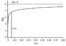
where $t_{1}$ ($=t_{0}e^{\frac{1}{2}\beta M_{1}}$) is the accumulation time of the main shock; $M_{2}$ in equation (34) is defined for $\left(1+e^{-bM_{1}}\right)^{r/2}-1<\tau/t_{1}<2^{r/2}-1$ ($0<M_{2}<M_{1}$). The function $M_{2}$ is plotted in Fig. 1 vs $\tau/t_{1}$ for $b=3.45$, $r=2/3$ ($\beta=2.3$) and $M_{1}=5$. For $\tau/t_{1}$ very close to zero the magnitude $M_{2}$ is vanishing, and for $\tau/t_{1}\longrightarrow 2^{r/2}-1$ the magnitude $M_{2}$ tends to $M_{1}$; the Bath partner occurs at $\tau_{0}/t_{1}\simeq\frac{1}{2}re^{-2\sqrt{2}/r}\simeq 5\times 10^{-3}$ with the magnitude $M_{2}=3.8$. The function $M_{2}(\tau/t_{1})$ is a very steep function, for the whole (reasonable) range of parameters; the whole accompanying seismic activity is, practically, concentrated in the lapse of time $\tau_{0}$. On the scale $\tau/t_{1}$ the pair probability of this activity is an abruptly increasing function of $M_{2}$. If we use $M_{2}$ given by equation (34) in the distribution $\frac{1}{2}\beta e^{-\frac{1}{2}\beta M_{2}}$ for small values of $\tau/t_{1}$, we get an Omori-type law, as expected (Apostol, 2006c).

Finally, we note that the aftershock (foreshock) magnitude $M_{2}$ given by equation (34) can be approximated by

$$M_{2}\simeq(1-r/2)M_{1}+\frac{1}{b}\ln\left(\frac{2\tau}{rt_{0}}\right)$$

(35)

for

$$\frac{1}{2}re^{-(1-r/2)bM_{1}}<\tau/t_{0}<\left(2^{r/2}-1\right)e^{\frac{1}{2}\beta M_{1}}\,\,\,,$$

(36)

where $t_{0}$ is the cutoff time. The lower bound $\frac{1}{2}rt_{0}e^{-(1-r/2)bM_{1}}$in equation (36) corresponds to a (very small) quiescence time elapsed from the occurence of the main shock ($M_{2}=0$). This time is much shorter than the cutoff time $t_{0}$, so, in fact, it is irrelevant. The cumulative fraction of aftershocks (foreshocks) with magnitude from zero to $M_{2}$ is $N_{cum}/N=1-e^{-\frac{1}{2}\beta M_{2}}$, where $N$ is the total number of aftershocks (foreshocks). Making use of equation (35) we get the cumulative fraction for time $\tau$

$$N_{cum}/N=1-\left(\frac{rt_{0}}{2\tau}\right)^{r/2}e^{-\frac{1}{2}(1-r/2)\beta M_{1}}\,\,.$$

(37)

This fraction is a rapidly increasing function of time, as it was pointed out recently by Ogata and Tsuruoka, 2016. The cutoff time, which is necessary in equation (37), remains an empirical parameter.

In foreshock-main shock-aftershock sequences of associated (accompanying) earthquakes we can discerne, in principle, two types of correlations. One type, which we call dynamical (or causal) correlations, imply an "interaction between earthquakes", i.e. an interaction between their focal regions (e.g., a static stress). Another type consists of purely statistical (or acausal) correlations, though both types have a statistical character. Dynamical correlations imply a variation (fluctuation) of the accumulation time, which is estimated by means of the geometric-growth model of energy accumulation in the focal region. This way, the number of dynamically correlated earthquakes is derived, as a statistical standard deviation, and the single-event distribution law for these earthquakes is deduced. It is a Gutenberg-Richter-type exponential law with the parameter $\beta$ changed into $\beta/2$. This change reflects a roll-off effect in the Gutenberg-Richter statistical distribution, related, mainly, to clusters with high-magnitude main shocks.

The correlations are discussed by means of the magnitude-difference distribution for earthquake pairs, where the difference in magnitude is extended to negative values. This distribution has a vanishing mean value of the magnitude difference, such that the foreshock-aftershock seismic activity appears as fluctuations in magnitude. The corresponding standard deviation is the average diference in magnitudes between the main shock and its greatest aftershock (foreshock). This difference in magnitude is given by $\Delta M=2\sqrt{2}/\beta$ for dynamically correlated earthquakes, which leads to $\Delta M=1.2$ for the reference value $\beta=2.3$ ($1$ for decimal logarithms). This is the Bath’s law. If we allow for purely statistical correlations the difference in magnitude is, approximately, $\Delta M=\sqrt{2}/\beta$. The difference between these two formulae and the variability of the parameter $\beta$ may explain the variability in the results of the statistical analysis of empirical data for $\Delta M$. We note that it is difficult to differentiate empirically between dynamical and purely statistical correlations. For earthquake clusters with moderate-magnitude main shocks the purely statistical correlations dominate. They lead to a Bath’s law $\Delta M=1/\sqrt{2}\beta$, which gives $\Delta M=0.31$ for the reference value $\beta=2.3$, indicating rather doublets as Bath’s partners.

The roll-off effect in the Gutenberg-Richter distribution and the presence of the dynamical correlations are also indicated by the pair (two-event, bivariate) distribution, which is derived by means of the geometric-growth model of energy accumulation. The same model is used to derive the deterministic time-magnitude correlations occurring in earthquake clusters. The time delay between the main shock and its largest aftershock (foreshock) is estimated; it is suggested to use this time interval as a criterion of estimating the temporal extension of the aftershock (foreshock) activity.

Acknowledgements

The author is indebted to the colleagues in the Institute of Earth’s Physics, Magurele, to members of the Laboratory of Theoretical Physics, Magurele, for many enlightening discussions, and to the anonymous reviewer for useful comments. This work was partially carried out within the Program Nucleu 2016-2019, funded by Romanian Ministry of Research and Innovation, Research Grant #PN19-08-01-02/2019. Data used for the fit (Vrancea region) have been extracted from the Romanian Earthquake Catalog, 2018. Part of them (period 1974-2004) are available through Apostol (2006a,b).

REFERENCES

Apostol, B. F. (2006a). A Model of Seismic Focus and Related Statistical Distributions of Earthquakes. Phys. Lett., A357, 462-466

Apostol, B. F. (2006b). A Model of Seismic Focus and Related Statistical Distributions of Earthquakes. Roum. Reps. Phys., 58, 583-600

Apostol, B. F. (2006c). Euler’s transform and a generalized Omori law. Phys. Lett., A351, 175-176

Apostol, B. F. & Cune, L. C. (2020). Short-term seismic activity in Vrancea. Inter-event time distributions. Ann. Geophys., to appear

Bath, M. (1965). Lateral inhomogeneities of the upper mantle. Tectonophysics, 2, 483-514

Bhattacharya, P., Chakrabarti, C. K., Kamal & Samanta, K. D. (2009). Fractal models of earthquake dynamics. Schuster, H. G. ed. Reviews of Nolinear Dynamics and Complexity pp.107-150. NY: Wiley.

Bullen, K. E. (1963). An Introduction to the Theory of Seismology. London: Cambridge University Press.

Console, R., Lombardi, A. M., Murru, M. & Rhoades, D. (2003). Bath’s law and the self-similarity of earthquakes. J. Geophys. Res., 108, 2128 10.1029/2001JB001651

Corral, A. (2006). Dependence of earthquake recurrence times and independence of magnitudes on seismicity history. Tectonophysics, 424, 177-193

Evison, F. (1999). On the existence of earthquake precursors. Ann. Geofis., 42, 763-770

Evison, F. & and Rhoades, D. (2001). Model of long term seismogenesis. Ann. Geophys., 44, 81-93

Felzer, K. R., Becker, T. W., Abercrombie, R. E., Ekstrom, G. & Rice, J. R. (2002). Triggering of the 1999 $M_{w}$ 7.1 Hector Mine earthquake by aftershocks of the 1992 $M_{w}$ 7.3 Landers earthquake., J. Geophys. Res., 107, 2190 10.1029/2001JB000911

Felzer, K. R., Abercrombie, R. E. & Ekstrom, G. (2004). A common origin for aftershocks, foreshocks and multiplets. Bull. Seism. Soc. Am., 94, 88-98

Felzer, K. R. & Brodsky, E. E. (2006). Decay of aftershock density with distance indicates triggerring by dynamic stress. Nature, 441,735-738

Frohich, C. & Davis, S. D. (1993). Teleseismic $b$ values; or much ado about $1.0$. J. Geophys. Res., 98, 631-644

Gutenberg, B. & Richter, C. (1944). Frequency of earthquakes in California, Bull. Seism. Soc. Am., 34, 185-188

Gutenberg, B. & Richter, C. (1956). Magnitude and energy of earthquakes. Annali di Geofisica, 9, 1-15 ((2010). Ann. Geophys., 53, 7-12

Hanks, T. C. & Kanamori, H. (1979). A moment magnitude scale. J. Geophys. Res., 84, 2348-2350

Helmstetter, A. & Sornette, D. (2003). Bath’s law derived from the Gutenberg-Richter law and from aftershock properties. Geophsy. Res. Lett., 30, 2069 10.1029/2003GL018186

Kanamori, H. (1977). The energy release in earthquakes. J. Geophys. Res., 82, 2981-2987

Kisslinger, C. (1996). Aftershocks and fault-zone properties. Adv. Geophys., 38 1-36

Kisslinger, C. & Jones, L. M. (1991). Properties of aftershock sequences in Southern California. J. Geophys. Res., 96, 11947-11958

Lavenda, B. H. & Cipollone, E. (2000). Extreme value statistics and thermodynamics of earthquakes: aftershock sequences. Ann. Geofis., 43, 967-982

Lay, T. & Wallace, T. C. (1995). Modern Global Seismology. San Diego, CA: Academic.

Lombardi, A. M. (2002). Probability interpretation of "Bath’s law. Ann. Geophys., 45, 455-472

Michael, A. J. & Jones, L. M. (1998). Seismicity alert probability at Parkfield, California, revisited. Bull. Seism. Soc. Am., 88, 117-130

Ogata, Y. & Tsuruoka, H. (2016). Statistical monitoring of aftershock sequences: a case study of the 2015 $M_{w}$7.8 Gorkha, Nepal, earthquake. Earth, Planets and Space, 68:44, 10.1186/s40623-016-0410-8

Papazachos, P. C. (1974). On certain aftershock and foreshock parameters in the area of Greece. Ann. Geofis., 24, 497-515

Pelletier, J. D. (2000). Spring-block models of seismicity: review and analysis of a structurally heterogeneous model coupled to the viscous asthenosphere. Rundle, J. B., Turcote, D. L. & Klein, W. eds. Geocomplexity and the Physics of Earthquakes. vol. 120. NY: Am. Geophys. Union.

Poupinet, G., Elsworth, W. L. & Frechet, J. (1984). Monitoring velocity variations in the crust using earthquake doublets: an application to the Calaveras fault, California. J. Geophys. Res., 89, 5719-5731

Purcaru, G. (1974). On the statistical interpretation of the Bath’s law and some relations in aftershock statistics. Geol. Inst. Tech. Ec. Stud. Geophys. Prospect. (Bucharest), 10, 35-84

Richter, C. F. (1958). Elementary Seismology (p.69). San Francisco, CA: Freeman.

Romanian Earthquake Catalogue (ROMPLUS Catalog). (2018). National Institute for Earth Physics, Romania.

Shearer, P. M. (2012). Self-similar earthquake triggering, Bath’s law, and foreshock/aftershock magnitudes: simulations, theory, and results for Southerm California. J. Geophys. Res., 117, B06310, 10.1029/2011JB008957

Stein, S. & Wysession, M. (2003). An Introduction to Seismology, Earthquakes, and Earth Structure. NY: Blackwell.

Tsapanos, T. M. (1990). Spatial distribution of the difference between magnitudes of the main shock and the largest aftershock in the circum-Pacific belt. Bull. Seism. Soc. Am., 80, 1180-1189

Udias, A. (1999). Principles of Seismology. NY: Cambridge University Press.

Utsu, T. (1969). Aftershocks and earthquake statistics (I,II): Source parameters which characterize an aftershock sequence and their interrelations. J. Fac. Sci. Hokkaido Univ., Ser. VII, 2, 129-195, 196-266

Utsu, T. (2002). Statistical features of seismicity. International Geophysics, 81, Part A, 719-732

Vere-Jones, D. (1969). A note on the statistical interpretation of Bath’s law. Bull. Seismol. Soc. Amer., 59, 1535-1541