Backpropagation on Dynamical Networks Supplementary Material

Appendix A Chaotic Oscillators Equations

Lorenz

	$\displaystyle\dot{x}_{i}$	$\displaystyle=\gamma(y_{i}-x_{i})+\sum_{i\neq j}c_{ij}(x_{j}-x_{i}),$
	$\displaystyle\dot{y}_{i}$	$\displaystyle=x_{i}(\rho-z_{i})-y_{i},$
	$\displaystyle\dot{z}_{i}$	$\displaystyle=x_{i}y_{i}-\beta z_{i},$

where $(\gamma,\beta,\rho)=(10,8/3,28)$ .

Chua

	$\displaystyle\dot{x}_{i}$	$\displaystyle=k(y_{i}-x_{i}+z_{i})+\sum_{i\neq j}c_{ij}(x_{j}-x_{i}),$
	$\displaystyle\dot{y}_{i}$	$\displaystyle=k\alpha(x_{i}-y_{i}\phi(y_{i})),$
	$\displaystyle\dot{z}_{i}$	$\displaystyle=k(-\beta x_{i}-\gamma z_{i}),$
	$\displaystyle\phi(y_{i})$	$\displaystyle=ay_{i}^{3}+by_{i},$

where $(k,\beta,\alpha,\gamma)=(-1,53.61,-0.75,17)$ .

Appendix B Recursive Partial Derivatives

The recursive relationship of the required partial derivatives for the backpropragation algorithm is given by:

	$\displaystyle\medmath{\left(\frac{\partial\mathbf{x}_{i}^{(1)}}{\partial c_{jk}}\right)_{t_{n}}}$	$\displaystyle=\medmath{\left[\frac{\partial\hat{F}(\mathbf{x}_{i}^{(1)})}{\partial c_{jk}}+\delta t\,\sum_{h\neq i}c_{ih}\frac{\partial g(\mathbf{x}_{i}^{(1)},\mathbf{x}_{h}^{(1)})}{\partial c_{jk}}\right}$
		$\displaystyle+\medmath{\left\frac{missing}{missing}{\partial c_{ih}}{\partial c_{jk}}g(\mathbf{x}_{i}^{(1)},\mathbf{x}_{h}^{(1)})\right]_{t_{n-1}},}$
	$\displaystyle\medmath{\left(\frac{\partial g(\mathbf{x}_{i}^{(1)},\mathbf{x}_{h}^{(1)})}{\partial c_{jk}}\right)_{t_{n-1}}}$	$\displaystyle=\medmath{\left[\frac{\partial g(\mathbf{x}_{i}^{(1)},\mathbf{x}_{h}^{(1)})}{\partial\mathbf{x}_{i}^{(1)}}\frac{\partial\mathbf{x}_{i}^{(1)}}{\partial c_{jk}}\right{}}$
		$\displaystyle+\medmath{\left\frac{missing}{missing}{\partial g(\mathbf{x}_{i}^{(1)},\mathbf{x}_{h}^{(1)})}{\partial\mathbf{x}_{h}^{(1)}}\frac{\partial\mathbf{x}_{h}^{(1)}}{\partial c_{jk}}\right]_{t_{n-1}},}$
	$\displaystyle\medmath{\left(\frac{\partial\hat{F}(\mathbf{x}_{i}^{(1)})}{\partial c_{jk}}\right)_{t_{n-1}}}$	$\displaystyle=\medmath{\left[\frac{\partial\mathbf{x}_{i}^{(1)}}{\partial c_{jk}}+\delta t\,\sum_{d}\frac{\partial f^{(1)}}{\partial\mathbf{x}_{i}^{(d)}}\frac{\partial\mathbf{x}_{i}^{(d)}}{\partial c_{jk}}\right]_{t_{n-1}},}$
	$\displaystyle\medmath{\left(\frac{\partial\mathbf{x}_{i}^{(2)}}{\partial c_{jk}}\right)_{t_{n-1}}}$	$\displaystyle=\medmath{\left[\frac{\partial\mathbf{x}_{i}^{(2)}}{\partial c_{jk}}+\delta t\,\sum_{d}\frac{\partial f^{(2)}}{\partial\mathbf{x}_{i}^{(d)}}\frac{\partial\mathbf{x}_{i}^{(d)}}{\partial c_{jk}}\right]_{t_{n-2}},}$
	$\displaystyle\medmath{\left(\frac{\partial\mathbf{x}_{i}^{(3)}}{\partial c_{jk}}\right)_{t_{n-1}}}$	$\displaystyle=\medmath{\left[\frac{\partial\mathbf{x}_{i}^{(3)}}{\partial c_{jk}}+\delta t\,\sum_{d}\frac{\partial f^{(3)}}{\partial\mathbf{x}_{i}^{(d)}}\frac{\partial\mathbf{x}_{i}^{(d)}}{\partial c_{jk}}\right]_{t_{n-2}},}$

where $\mathbf{x}_{i}^{(d)}$ corresponds to the $d$ ^th component of the state of node $i$ . Similarly, $f^{(d)}$ is the $d$ ^th component of the local dynamics function and $\hat{F}$ corresponds to the local dynamics contribution of the forward evolution,

\hat{F}(\mathbf{x}_{i}(t_{n}))=x_{i}(t_{n})+\delta t\;\hat{\dot{\mathbf{x}}}_{i}(t).

(2)

Appendix C Other Tested Networks

C.1 FitzHugh-Nagumo Neuron Network

An additional system consisting of a network of FitzHugh-Nagumo neuron oscillators [hong2011synchronization] was used to test the capabilities of the backpropagation regression method.

The neuron network presents an additional challenge when constructing a data-driven model due to the presence of disparate time scales in the dynamics (fast spiking depolarisation and slow repolarisation). It also demonstrates the performance of the backpropagation method in a more realistic context, i.e. the inference of neuronal networks. We focus on the FitzHugh-Nagumo system operating under a chaotic regime as given by Hong [hong2011synchronization] with equations,

	$\displaystyle\dot{V}$	$\displaystyle=V(V-1)(1-b_{1}V)-w+\frac{\alpha I}{\omega},$
	$\displaystyle\dot{w}$	$\displaystyle=b_{2}V,$
	$\displaystyle\ddot{I}$	$\displaystyle=-\omega^{2}I,$

with constant parameters $(\alpha,b_{1},b_{2},\omega)=(0.1,10,1,0.8105)$ . Diffusive coupling was applied on $V$ with coupling weights normally distributed with $(\mu,\sigma^{2})=(0.15,0.02^{2})$ and coupling probability $\log(N)/N$ and integration timestep $dt=0.02$ .

Refer to caption — Figure 1: Regression results for the FitzHugh-Nagumo neuron network with normally distributed coupling weights $(\mu,\sigma^{2})=(0.15,0.02)$ and connection probability $p$ over 80 iterations.

C.2 Heterogeneous Networks

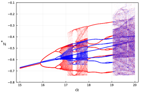
The formulation of the backpropagation regression algorithm assumes that the local dynamics $f$ for all nodes are identical. Whilst this is a useful property, this strong assumption is unlikely to be present in real systems. In many cases, nodes in a dynamical network may exhibit slight differences in their local dynamics. To test the effect network heterogeneity on regression performance, a 16 node Chua oscillator network was simulated with slightly differing bifurcation parameters for each node. We use the Chua system for this investigation, as it shows similar chaotic dynamics for a wide parameter range (see Figure 3).

The Chua system contains multiple coexisting attractors for particular values of the bifurcation parameter $\alpha$ [kengne2017dynamics]. When operating in the single scroll regime ( $\alpha\in[17,17.3]$ ), the isolated Chua system exhibits two separate chaotic attractors corresponding to the two scrolls. These two scrolls eventually merge into the characteristic double scroll Chua attractor for larger values of $\alpha$ (see Figure 3).

To simulate a heterogeneous network, the $\alpha$ parameter for each node in the network was randomly perturbed by an additional amount $\epsilon_{\alpha}\sim U(0,\xi_{\alpha})$ where $\xi_{\alpha}\in[0,0.3]$ . The backpropagation regression algorithm was tested on 7 different configurations of increasing $\xi_{\alpha}$ . Each configuration was tested on 8 randomly initialised 16 node Chua dynamical networks, with 40 regression iterations in each case.

The weight error performance was found to be robust to increasing levels of heterogeneity in network dynamics (see Figure 4). The effect of weight filtration was also found to be unchanged with increasing heterogeneity. However, increasing heterogeneity $\xi_{\alpha}$ resulted in a gradual decrease in the mutual information of local model predictions (see Figure 5). The backpropagation algorithm assumes that all nodes have identical local dynamics. Heterogeneity in node dynamics results in uncertainty the true model parameters when regressing the local model in the training and refitting stage. Mutual information was also tested against the control case where the model is exactly known, but evaluated with perturbed initial conditions $(\xi_{0}=0.005)$ .

Appendix D Backpropagation Algorithm Hyperparameters

A list of hyperparameters for the algorithm are provided in Table I. The selection of hyperparameter values require experimentation and were selected based on values typically used for BPTT training of RNNs. As a general guide, $K_{init}$ affects the degree of averaging in the mean field approach when estimating the vector field of the local dynamics $\hat{f}$ during initialisation. The parameters $N_{epochs}$ and $N_{refit}$ directly control the amount of time spent in stage of backpropagation and retraining. The learning rates $\eta$ and $\eta^{\prime}$ are used for the training the feedforward neural network local dynamics model. Selection of these values follow the same heuristics used for machine learning function approximation with the additional criteria that $\eta^{\prime}<\eta$ to ensure that the local dynamics model does not change too much in each refit iteration. The parameters $\bar{\alpha},\beta,d_{eff}$ and $r$ are defined similarly to those normally used in regression and learning rate scheduler of regular BPTT training RNNs. The freerun prediction length $t_{in}$ alters the length of the trajectory used to calculate the errors for backpropagation. Larger $t_{in}$ allow the accumulation of errors over time and prioritises the adjustment of weights that have a larger impact on prediction performance, resulting in better convergence and stability at the expense of computational speed. However, $t_{in}$ should be selected to be smaller than the natural Lyapunov time scale of the system to prevent instability.

Hyper-parameter	Value	Description
$K_{init}$	8	Number of neighbours in mean field approach for initial model training
$N_{epochs}$	30	Number of training epochs used in each neural network model training run
$N_{refit}$	40	Number of backpropagation-decoupling-refit alternations to run
$\eta$	0.001	Model training learning rate
$\eta^{\prime}$	0.0002	Model refit learning rate
$\bar{\alpha}$	0.0005	Average learning rate for of each coupling weight in the $\hat{C}$
$\beta$	0.9	Learning rate momentum parameter
$t_{in}$	10	Length of freerun predictions used to calculate and backpropagate error
$d_{eff}$	0.98	Effective learning rate decay after each decay-reset cycle in scheduler
$r$	2.0	Amount to multiply decreased learning rate at the end of decay-reset cycle

TABLE I: List of hyperparameters

Notable Hyperparameters

The backpropagation algorithm requires the selection of various hyperparameters that govern the regression behaviour.

•

Momentum ( $M$ ) - This quantity includes a notion of momentum in the gradient update by allowing previous calculated update steps to propagate into future steps with a decaying effect. This technique is also commonly used in RNN backpropagation to improve convergence,

$d\hat{C}(n+1)=M\,d\hat{C}(n-1)+(1-M)\,d\hat{C}(n).$ (3)
•

Model Learning Rate ( $\eta$ ) - The step size of the feedforward network during the initial construction of the model and retraining.
•

Node Learning Rate ( $\bar{\alpha}$ ) - The average learning rate that would be applied to each coupling weight if all real links weights are equal in the calculated gradient and exist with probability $p$ . Its relationship to the real learning rate is given by,

$\alpha_{LR}=\sqrt{p\cdot\frac{N(N-1)}{2}\cdot\bar{\alpha}}.$ (4)
•

Input History Length ( $t_{in}$ ) - The amount of steps over which to unfold the backpropagation regression algorithm. Longer history results in the accumulation of coupling weight effects over a longer period and provides better convergence at the cost of slower computation.