Axial spectral encoding of space-time wave packets
Abstract
Space-time (ST) wave packets are propagation-invariant pulsed optical beams whose group velocity can be tuned in free space by tailoring their spatio-temporal spectral structure. To date, efforts on synthesizing ST wave packets have striven to maintain their propagation invariance. Here, we demonstrate that one degree of freedom of a ST wave packet – its on-axis spectrum – can be isolated and purposefully controlled independently of the others. Judicious spatio-temporal spectral amplitude and phase modulation yields ST wave packets with programmable spectral changes along the propagation axis; including red-shifting or blue-shifting spectra, or more sophisticated axial spectral encoding including bidirectional spectral shifts and accelerating spectra. In all cases, the spectral shift can be larger than the initial on-axis bandwidth, while preserving the propagation-invariance of the other degrees of freedom, including the wave packet spatio-temporal profile. These results may be useful in range-finding in microscopy or remote sensing via spectral stamping.
I Introduction
The unique opportunities offered by jointly manipulating the spatial and temporal degrees of freedom of an optical field – rather than modulating the field separately in space [1] or time [2] – have started recently to capture considerable attention [3, 4, 5, 6, 7, 8, 9, 10]. One example within this general enterprise is that of ‘space-time’ (ST) wave packets, which are a class of pulsed beams endowed with a spatio-temporal structure in which each spatial frequency is associated with a single wavelength [11, 12, 13], by virtue of which they exhibit unique characteristics; e.g., propagation-invariance [7, 12, 14, 15, 16, 17, 18], controllable group velocities [6, 19, 20, 21], self-healing [22], and omni-resonant interaction with planar cavities [23, 24]. Although the study of propagation-invariant pulsed beams extends for almost 40 years [25, 26, 27, 28, 29, 30], the focus has always been on maintaining the field invariant rather than controlling the axial variation of one characteristic while maintaining the others fixed. We pose here the following question: can a ST wave packet remain propagation-invariant while controlling the axial evolution of one of its aspects in isolation from all the other characteristics of the wave packet? For example, can we control the evolution of the on-axis spectrum of a ST wave packet without impacting its propagation invariance or the tunability of its group velocity? This would produce a continuous, axial spectral encoding that can be useful in range-finding through spectral stamping of reflections from objects at different distances – whether in the context of optical microscopy or remote sensing.
Recently, an alternative approach to tuning the group velocity of an optical wave packet known as the ‘flying-focus’, which does not provide diffraction-free behaviour, was proposed theoretically [31] and demonstrated experimentally [32, 33]. This approach relies on longitudinal chromatism in which a temporally chirped pulse is focused by a lens having prescribed chromatic aberrations. In this strategy, the on-axis spectrum shifts continuously with propagation, but this shift is not independent of the group velocity; in fact, the rate of the spectral shift dictates the group velocity of the flying-focus. In other words, the group velocity and the axial evolution of the spectrum are inextricably linked and cannot be manipulated independently. This helps sharpen the question posed above: can we control the spectral evolution and the group velocity of a wave packet independently through sculpting its spatio-temporal structure? More generally, can we produce an arbitrary axial spectral encoding for an optical wave packet while maintaining its other desirable characteristics (e.g., propagation-invariance) intact?
Here we show that ST wave packets can support controllable and readily adaptable evolution of the on-axis spectrum along the propagation direction. Such axial spectral encoding includes red-shifting or blue-shifting spectra, complex bidirectional-shifting spectra in which the direction of the spectral shift can switch at prescribed axial locations, and accelerating spectra. This control can be exercised independently of the wave-packet group velocity (whether subluminal or superluminal), and without affecting its propagation invariance. Time-resolved measurements of the ST wave packet confirm that its spatio-temporal profile remains invariant with propagation despite the underlying spectral changes. Our approach is independent, in principle, of the selected wavelength [34] or bandwidth [35] of the field. These features are achieved through sculpting the amplitude and phase distribution imparted to the spectrally resolved wave front, in contrast to our previous work that made use of purely phase modulation to synthesize propagation-invariant ST wave packets [13]. Our results highlight a crucial aspect of modulating the joint spatio-temporal spectrum rather than manipulating the spatial (Fourier optics [1]) or the temporal (pulse shaping [2]) degrees of freedom separately. Indeed, whereas spectral phase modulation is a staple of ultrafast pulse shaping, spectral amplitude modulation would result in irrecoverable spectral filtering, and is hence usually avoided. Uniquely, joint spatio-temporal spectral amplitude modulation can be utilized without necessarily filtering or eliminating any portion of the temporal spectrum. This strategy opens up a plethora of opportunities for programmable axial spatial encoding of ST wave packets – independently of the wave-packet group velocity, extending from range-finding in microscopy and remote sensing, to nonlinear interactions in plasmas [36, 37].
II Space-time wave packets
The concept of propagation-invariant ST wave packets is by now well-established [12, 21, 13], and we provide here only a brief overview to lay the groundwork for the subsequent formulation of axial spectral encoding. Such a wave packet in free space is a pulsed optical beam whose spatio-temporal spectral support domain lies along the intersection of the light-cone with a tilted spectral plane ; where and are the transverse and longitudinal components of the wave vector along and , respectively, is the temporal (angular) frequency, is the speed of light in vacuum, is a fixed temporal frequency, is the corresponding wave number, and is the angle made by the spectral plane with respect to the -axis [Fig. 1(a)]. We refer to as the spectral tilt angle and to as the spatial frequency. Such a field can be shown to have a propagation-invariant envelope that travels rigidly in free space at a group velocity independently of beam size, pulse width, or central wavelength – as demonstrated recently [19]. Indeed, the spectral projection onto the -plane is a straight line, indicating absence of group velocity dispersion [Fig. 1(a)]. The projection onto the -plane is a conic section [38] that can be approximated by a parabola for narrow temporal bandwidths , indicating that each spatial frequency is associated with a single temporal frequency [Fig. 1(a)]:
| (1) |
Tuning the group velocity requires changing the curvature of this spatio-temporal spectral parabola, which can be readily achieved via phase-only spectral modulation [19, 20, 13].

Such a ST wave packet can be prepared via the two-dimensional pulse synthesizer depicted in Fig. 1(b) starting with femtosecond pulses from a Ti:sapphire laser (Tsunami, Spectra Physics) having a central wavelength nm and a pulse duration of fs (as verified via a FROG measurement [39] obtained by a GRENOUILLE [40] commercial platform). The spectrum of the plane-wave (30-mm-diameter) pulses are spread in space by a diffraction grating (1200 lines/mm; Newport 33009FL01-360R) and collimated by a cylindrical lens before impinging on a spatial light modulator (SLM; Hamamatsu X10468-02). The SLM imparts a two-dimensional phase distribution to the spatially resolved spectrum, which is then retro-reflected through the lens and reconstituted by the grating to produce the ST wave packet [Fig. 1(b)]. The SLM-imparted phase distribution [Fig. 2(a)] can be designed to implement any spectral tilt angle by assigning to each wavelength incident on the SLM a phase distribution corresponding to a particular spatial frequency according to Eq. 1 [12, 13]. In all cases, a spatial filter (in the form of a low-pass rejection filter to eliminate the spatial components in the immediate vicinity of ) is placed in the Fourier plane between two cylindrical lenses with their focusing axis parallel to the -coordinate, to remove any non-diffracted portion of the field (due to the finite diffraction efficiency of the SLM).
We characterize the synthesized ST wave packets in three domains [Fig. 1(b)]. (1) A CCD camera (TheImagingSource DMK 33UX178) is scanned along the -axis in the path of the ST wave packet to record the time-averaged intensity . (2) A 400-m-diameter multimode fiber (Thorlabs, M74L01- m, 0.39 NA), connected to an optical spectrum analyzer (OSA; Advantest q8381, 0.1-nm-resolution), is scanned along the -axis to record the axial spectral evolution of the ST wave packet . A multimode is selected to increase the signal-to-noise ratio and thus confirm the predicted effect unambiguously. The diameter was selected to capture a large portion of the field energy around the optical axis and thus avoid any spurious spectral effects that can arise if a single-mode fiber is used instead. The measured spectrum is thus representative of the axial field evolution. However, the multimode fiber introduces spectral broadening compared to a single-mode fiber, and the results reported here are therefore a conservative underestimate of the axial spectral encoding offered by our approach. (3) The spatio-temporal profile of the ST wave packet is measured by interfering the wave packet with the original Ti:sapphire laser pulses at any selected axial plane . By placing the pulse synthesizer in one arm of a Mach-Zehnder interferometer, and placing an optical delay in the reference arm traversed by the femtosecond pulses, time-resolved measurements are obtained from the visibility of the spatially resolved interference fringes that are observed when the ST wave packet and the reference pulse overlap in space and time. This arrangement is also used to estimate the group velocity of the ST wave packet [19, 20, 21].

. (b) Calculated time-averaged intensity for propagation-invariant (left) and axial spectral encoded (right) ST wave packets. Note the very different axial and transverse spatial scales. (c) Calculated spectral evolution for the ST wave packets in (b). (d) Spectra at selected axial planes for the ST wave packets in (b). The spectrum of the propagation-invariant ST wave packet (left) does not change significantly with propagation, whereas that of the axially spectral-encoded ST wave packet (right) undergoes significant spectral evolution with propagation.
III Space-time wave packets with axial spectral encoding
An example of the phase distribution imparted by the SLM to realize a ST wave packet is shown in Fig. 2(a), corresponding to a spectral tilt angle (superluminal group velocity ) [12]. Implementing such a phase distribution results in a diffraction-free beam [Fig. 2(b)] whose spectrum is invariant [Fig. 2(c-d)] over its propagation length. We proceed to show that the key to controlling the axial spectral evolution of the wave packet is modulating the amplitude of its spatio-temporal spectrum at the SLM plane – a degree of freedom that has hitherto gone unexploited.
Note that the amplitude modulation is not introduced by means of an additional device or component. Rather, the SLM serves as a phase and amplitude modulator. The continuous sections of the SLM where the phase is set to zero produce a field whose spatial spectrum is in the vicinity of , which is then eliminated by the spatial filter (SF) along with the non-diffracted field from the SLM.
Consider the configuration shown in Fig. 2(a) where we combine the phase distribution (corresponding to a particular spatial tilt angle ) with a two-dimensional amplitude masking distribution . Consequently, the phase modulation imparted by the SLM is now restricted to a particular portion of the spectrally spread wave front as dictated by the amplitude mask, . Experimentally, this amplitude modulation is achieved by setting the SLM phase to zero wherever the target amplitude is required to be zero, and then subsequently inserting a spatial filter in the Fourier plane between the cylindrical lenses L2-x and L3-x placed in the path of the ST wave packet [Fig. 1(b)] to eliminate the unscattered (or zero-phase) field component.
From Fig. 2(a) we can understand why joint spatio-temporal spectral amplitude modulation does not necessarily eliminate a wavelength altogether as it would in a traditional ultrafast pulse shaper that relies solely on temporal spectral modulation. Because each column in as shown in Fig. 2(a) is associated with a single wavelength, the full spectral bandwidth remains intact as long as the two-dimensional spatio-temporal spectral amplitude modulation does not eliminate any whole column. Instead, amplitude modulation here leads to a change in the axial distribution of each wavelength. In contrast, in traditional pulse shaping [2], the two-dimensional distribution in Fig. 2(a) is collapsed to one dimension, so that amplitude modulation would inevitably eliminate wavelengths altogether from the spectrum.
Choosing for the transverse coordinate in the plane of the SLM and in the observation plane at axial position [Fig. 1(b)], the freely propagating field (the cylindrical lens L1-y affects the field only along ) is given by the usual Fresnel integral:
| (2) |
where is the field at the SLM along a single column (one temporal frequency ), and is the product of a linear phase imparted by the SLM and two constant amplitude windows centered at of width ,
| (3) |
here both and change with , is a rectangular (constant) function of width centered at , and is the spectral amplitude for the temporal frequency ; in our experiments is approximately constant independently of . It is understood throughout that , which is obtained by inverting Eq. 1. From this formulation, we can immediately make two conclusions. First, the field associated with the frequency has its on-axis peak at
| (4) |
Second, the transverse width over which the field is spread at is
| (5) |
where . From these two observations, we can reverse engineer the amplitude mask at the SLM plane by determining and required to localize the temporal frequency at the specific location or locations along .
By applying this algorithm to all the frequencies modulated by the SLM, thereby sculpting the amplitude mask , we can realize an arbitrary axial spectral encoding for the ST wave packet over any desired bandwidth and along a specified axial range . The spatio-temporal profile of the ST wave packet endowed with the desired axial spectral encoding is thus obtained after integrating over the temporal bandwidth:
| (6) |
After implementing the amplitude mask shown in Fig. 2(a), the time-averaged intensity remains diffraction-free for an extended distance, but additional transverse sidelobes appear [Fig. 2(b)]. These sidelobes are a consequence of the rectangular-shaped amplitude filter at each temporal frequency; applying a Gaussian amplitude modulation can smooth out these sidelobes.
The axial spectral encoding can be ascertained by examining the evolution of the spectrum along the propagation axis. The axial spectrum is integrated over the transverse extent shown in Fig. 2(b), from m to m (corresponding to the diameter of the multimode fiber used in our experiments to collect the spectrum), to yield , which we plot in Fig. 2(c). For propagation-invariant ST wave packets produced via phase-only modulation, the spectrum remains mostly constant up to mm. The short-wavelength end of the spectrum gradually diminishes beyond mm [Fig. 2(c)], which accompanies departure from the diffraction-free condition [Fig. 2(b)]. The ST wave packet simulated in Fig. 2 is superluminal (, ) [38]. Selecting a subluminal ST wave packet instead (, ) would result in a diminishing of the long-wavelength portion of its spectrum at the end of the propagation distance.
In contrast, the axial spectral evolution for the ST wave packet after amplitude-masking clearly shows an axial spectral encoding with propagation [Fig. 2(c)]: the spectrum at any axial plane is narrow compared to that of the propagation-invariant ST wave packet, and it undergoes a significant red-shift along . This behavior is further highlighted by comparing the spectrum at selected axial planes for both wave packets in Fig. 2(d). In the case of the axially spectral-encoded ST wave packet, the spectral shift along results in disjoint spectra at the axial start and end points.
IV Experiment
We have carried out a sequence of experiments that demonstrate multiple axial spectral encodings for ST wave packets through amplitude-masked phase-modulation of the spatio-temporal spectrum. In each experiment, we measure the axial intensity profile , and the axial spectral evolution integrated along over a fixed transverse width m (as determined by the diameter multimode fiber collecting the signal).
IV.1 Synthesizing axially red-shifting spectra
As an initial proof-of-concept, we implemented the amplitude-masked phase distributions depicted in Fig. 3(a) corresponding to two red-shifting spectra (the spectrum shifts from shorter to longer wavelengths along ). The spectral tilt angle here is , and the two amplitude masks and are designed to yield different axial red-shifting rates. Whereas the width of the amplitude window is a constant , the center of the window moves along a linear trajectory creating a wedge-shaped mask: .
In the first example [ in Fig. 3, left column], we set nm and nm, and select to produce a measured average on-axis FWHM spectral bandwidth of nm. As noted earlier, the measured spectrum when utilizing a multimode fiber to couple light into the OSA is broadened by in all cases in comparison with that obtained by using a single-mode fiber. The results reported here are thus a conservative underestimate of the spectral tuning capability of this strategy. The overall shift of the center wavelength of the axial spectral encoding is nm over a distance of mm, resulting in an axial red-shifting rate of pm/mm. This is only a first-order estimate because the axial spectral encoding is not linear along . A linear axial encoding requires implementing a different amplitude mask (see confirmation of this point below). The time-averaged intensity is provided in the Supplementary Material, and is in excellent agreement with the simulation in Fig. 2(b).
In the second example [ in Fig. 3, right column], we reduce the axial red-shifting rate to pm/mm by selecting a sharper slope of the amplitude mask whereupon nm, nm, while maintaining the same value for . In this case, the shift in the center wavelength of the axial spectral encoding is nm observed over a distance of mm. The spectra at selected axial planes are plotted for these two examples in Fig. 3(c). As a point of reference, we provide a Supplementary Movie (Movie10) for the spectral evolution of the ST wave packet with the amplitude mask removed, which shows a mostly invariant axial spectrum. Supplementary Movies corresponding to the amplitude masks and (Movie1 and Movie2, respectively) display the change in the spectral encoding along . Together, these two examples provide a demonstration of the general control strategy over the rate of axial spectral shift.
IV.2 Synthesizing axially blue-shifting spectra
Next we demonstrate that the same approach is applicable to blue-shifting axial spectral encoding (the spectrum shifts from longer to shorter wavelengths along ). The designed amplitude masks for two different axial blue-shifting rates are shown in Fig. 4(a). The slope of the wedge-like amplitude mask has the opposite sign of the red-shifting masks in Fig. 3(a). Here the underlying phase distribution corresponds to a subluminal spectral tilt angle of . In the first example ( in Fig. 4,left column) a blue-shifting spectral rate of pm/mm is achieved, corresponding to a total spectral shift of nm over mm; and in the second example ( in Fig. 4, right column) pm/mm, corresponding to nm over mm; see Fig. 4(b,c). These values approximately mirror the rates observed in the red-shifting scenario in Fig. 3. The measured time-averaged intensity is given in the Supplementary Material. Supplementary Movies corresponding to the amplitude masks and (Movie3 and Movie4, respectively) display the measured change in the spectral encoding along .


IV.3 Synthesizing axially bidirectional-shifting spectra
The axial spectral encodings in the previous subsections all feature monotonic (or uni-directional) spectral shifts. However, our approach is more general and, in principle, can establish arbitrary evolution of the on-axis spectrum. In Fig. 5(a), we show the amplitude-masked phase distributions required to produce axial spectral encodings that feature nonmonotonic (here, bidirectional) spectral shifts. In one example ( in Fig. 5(a), left column), the amplitude mask is designed to result initially in a blue-shift (from nm to nm over mm) followed by a red-shift (from nm to nm over mm). The measured axial spectral evolution is plotted in Fig. 5(b) along with the spectra at selected axial planes. In the second example ( in Fig. 5(a), right column), the amplitude mask is designed to result initially in a red-shift (from nm to nm over mm) followed by a blue-shift (from nm to nm over mm); see Fig. 5(b,c) for the measured . Supplementary Movies corresponding to the amplitude masks and (Movie5 and Movie6, respectively) display the change in the spectral encoding along .
IV.4 Synthesizing an axially arbitrary-shifting spectrum

In the three classes of axial spectral encoding provided above (red-, blue-, and bidirectional-shifting), the amplitude-masked phase distributions implemented by the SLM in Fig. 1(b) feature wedge-like masks with a linear slope for . As seen in Fig. 3-Fig. 5, such amplitude masks result in a nonlinear trajectory of the axial spectral evolution.
In order to exercise precise control over the axial spectral encoding, we construct a predictive theory for its quantitative dependence on the amplitude mask shape. To enforce a specific axial spectral encoding characterized by an on-axis spectral profile over a particular stretch of the -axis, Eqs. 1, 3, and 4 allow us to establish the following relationships for the amplitude-mask:
| (7) |
These equations provide a one-to-one correspondence between the position of the amplitude modulation and the axially realized wavelength. Making use of these equations, we realize the sophisticated axial spectral encodings plotted in Fig. 6. First, we demonstrate the linear axial spectral encoding plotted in Fig. 6(a), in contrast to those in Figs.3-5, using an amplitude mask that follows a supra-linear pattern rather than a linear one. Second, we accelerate the axial spectral encoding in Fig. 6(b) by relying on an amplitude mask with a sub-linear pattern. Finally, we show in Fig. 6(c) an example of an axial spectral encoding featuring a spectral discontinuity comprising a blue-shifting axial section, followed by a step to a red-shifting axial section, with a spectral gap separating the two sections produced by the amplitude mask . We provide in the Supplementary Materials the exact equations for the amplitude masks shown in Fig. 6. Supplementary Movies corresponding to the amplitude masks , , and (Movie7, Movie8, and Movie9 respectively) display the change in the spectral encoding along .
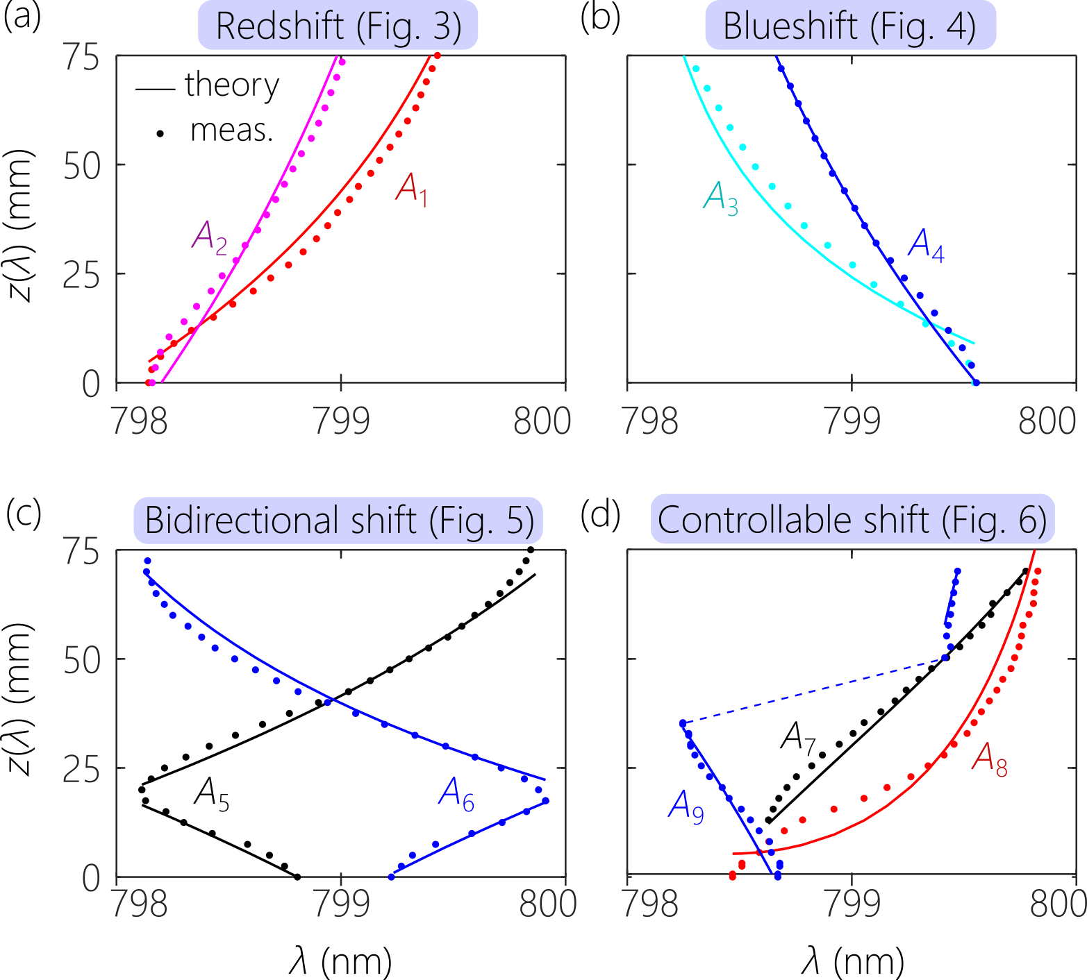
We summarize in Fig. 7 the axial spectral encodings demonstrated in Figs. 3-6: red-shifting spectra in Fig. 7(a), blue-shifting spectra in Fig. 7(b), bidirectional spectra in Fig. 7(c), and the precisely controlled spectral encodings from Fig. 6 in Fig. 7(d). In each case, we plot the data in the form of the center of a Gaussian distribution fitted to the spectrum at each axial position . With each data set, we plot the axial spectral encoding predicted based on Eq. IV.4 (see Supplementary Materials). We find excellent agreement between the data and the predictions in all cases.
V Time-Resolved Measurements
We have so far presented time-averaged spectral measurements of the evolution of the on-axis spectrum for the synthesized ST wave packets. In this Section, we present time-resolved measurements of their spatio-temporal profiles in comparison with those of propagation-invariant ST wave packets. We aim from these measurements to show that the amplitude-masking of the phase modulation does not impact the wave packet group velocity.
We determined the group velocity of a ST wave packet by measuring its relative group delay with respect to a reference pulse traveling at ; see [19, 20, 21]. We plot in Fig. 8(a) the spatio-temporal profiles at three axial planes (, 10, and 30 mm) for two ST wave packets both having (). One ST wave packet was synthesized via phase-only spectral modulation and is thus propagation invariant [Fig. 8(a)], and the other via the amplitude-masked phase modulation from Fig. 3(a) that produces a red-shifting axial spectral encoding [Fig. 8(b)]. The width of the wave packet at the center of its spatial profile is smaller for the propagation-invariant ST wave packet in comparison with its axial spectrally encoded counterpart, as expected because of its broader spectrum.

We plot in Fig. 8(c) the spectrum at the three axial planes , 10, and 30 mm. The 2-nm-bandwidth spectra for the propagation-invariant ST wave packet are unchanged with , whereas the narrower spectra for the axially spectral-encoded ST wave packet red-shifts with . The narrower spectrum of the latter results in a broad temporal profile [Fig. 8(b)]; whereas the broad spectrum of the propagation-invariant ST wave packet results in a narrow temporal profile [Fig. 8(a)]. In both cases however, the spatio-temporal profile is preserved over the propagation distance.
In Fig. 8(d) we plot the ST wave packet temporal profiles at the beam center measured at , 10, and 30 mm. The initial measurement at is the reference point for measuring subsequent group delays. Crucially, the group delays incurred by both wave packets are equal at the two planes and 30 mm, thereby proving that amplitude-masking does not impact the group velocity. At mm the group delay is ps and at mm is ps, which are consistent with a group velocity of (note that this superluminal group velocity does not contradict relativistic causality [41, 42, 43, 21]).
Finally, besides confirming that amplitude-masking does not impact the group velocity of the ST wave packet, we have also verified that the same axial spectral encoding can be implemented using ST wave packets of different group velocity. We present the data in the Supplementary Materials measurements of the axial spectral evolution of wave packets with () and () using the same amplitude mask that induces a red-shifting axial spectrum.
VI Discussion and Conclusion
The added feature of axial spectral encoding demonstrated here with ST wave packets can now be combined with previous achievements made utilizing these unique pulsed beams, such as long-distance propagation [15, 16] and self-healing [22]. One can now potentially rely on the wavelength of light reflected from an object as an axial-ranging stamp; that is, the wavelength of the reflected or scattered light will correlate with the object’s position and thus indicate its distance from the source. Because ST wave packets can be synthesized with narrow transverse widths ( m in [12] and m in [23]) and large depths of focus (25 mm for the 7-m-wide wave packet in [12]), they can be useful in the context of optical microscopy. Alternatively, the demonstration of propagation lengths approaching 100 m with ST wave packets [16] suggests the possibility of implementing such a protocol in remote sensing. Moreover, the experiments reported here for axial spectral encoding all made use of coherent ultrafast laser pulses. However, such effects can also be achieved with incoherent light from a LED [44] or superluminescent LED [45].
We are now in a position to compare the two major strategies for creating optical wave packets of controllable group velocity in free space: the flying-focus approach [31, 32, 33] and ST wave packets. The flying-focus strategy produces wave packets that are not diffraction-free but whose spectrum evolves monotonically along the propagation axis, and this spectral evolution determines the group velocity of the wave packet. The spectral evolution and the group velocity are not independently addressable in this case. On the other hand, ST wave packets are diffraction-free and have controllable group velocities that can be tuned by tailoring their spatio-temporal structure via spectral-phase-only modulation. The spectrum of such a wave packet is also propagation-invariant. However, we have shown here that by exploiting an amplitude-masked spectral-phase modulation the on-axis spectrum can be made to evolve with arbitrary axial profiles, whether monotonic or non-monotonic, independently of the group velocity while maintaining the propagation-invariance of the wave packet.
In conclusion, we have presented a comprehensive scheme for controlling the evolution of the on-axis spectrum of a freely propagating ST wave packet: the group velocity and the axial spectral evolution are arbitrary and tuned independently, while maintaining propagation invariance. Using this approach, we have produced axial spectral encodings in the form of red-shifting, blue-shifting, bidirectional spectral shifting (blue-shifting followed with red-shifting or vice versa over prescribed axial distances), and controlled rates of spectral shifts (linear or accelerating). This scheme is equally applicable to coherent ultrafast pulses and to broadband incoherent stationary fields. Unlike previous efforts on ST wave packets over the past years that have been devoted to maintaining their propagation invariance, we have demonstrated here that one degree of freedom (the on-axis spectrum) can be isolated and control of its axial propagation exercised while retaining the propagation-invariance of its other degrees of freedom. These results may be useful in spectral stamping for axial range-finding in microscopy and remote-sensing.
Acknowledgments. We thank G. Li and P. J. Delfyett for loan of equipment. This work was funded by the U.S. Office of Naval Research (ONR) contracts N00014-17-1-2458 and N00014-19-1-2192, and ONR MURI contract N00014-20-1-2789.
References
- Goodman [2005] J. W. Goodman, Fourier Optics (Roberts & Company, 2005).
- Weiner [2009] A. M. Weiner, Ultrafast Optics (John Wiley & Sons, Inc., 2009).
- Kondakci and Abouraddy [2016] H. E. Kondakci and A. F. Abouraddy, Diffraction-free pulsed optical beams via space-time correlations, Opt. Express 24, 28659 (2016).
- Parker and Alonso [2016] K. J. Parker and M. A. Alonso, The longitudinal iso-phase condition and needle pulses, Opt. Express 24, 28669 (2016).
- Wong and Kaminer [2017a] L. J. Wong and I. Kaminer, Abruptly focusing and defocusing needles of light and closed-form electromagnetic wavepackets, ACS Photon. 4, 1131 (2017a).
- Wong and Kaminer [2017b] L. J. Wong and I. Kaminer, Ultrashort tilted-pulsefront pulses and nonparaxial tilted-phase-front beams, ACS Photon. 4, 2257 (2017b).
- Porras [2017] M. A. Porras, Gaussian beams diffracting in time, Opt. Lett. 42, 4679 (2017).
- Efremidis [2017] N. K. Efremidis, Spatiotemporal diffraction-free pulsed beams in free-space of the Airy and Bessel type, Opt. Lett. 42, 5038 (2017).
- Shaltout et al. [2019] A. M. Shaltout, K. G. Lagoudakis, J. van de Groep, S. J. Kim, J. Vuc̆ković, V. M. Shalaev, and M. L. Brongersma, Spatiotemporal light control with frequency-gradient metasurfaces, Science 365, 374 (2019).
- Chong et al. [2020] A. Chong, C. Wan, J. Chen, and Q. Zhan, Generation of spatiotemporal optical vortices with controllable transverse orbital angular momentum, Nat. Photon. 14 (2020).
- Donnelly and Ziolkowski [1993] R. Donnelly and R. Ziolkowski, Designing localized waves, Proc. R. Soc. Lond. A 440, 541 (1993).
- Kondakci and Abouraddy [2017] H. E. Kondakci and A. F. Abouraddy, Diffraction-free space-time beams, Nat. Photon. 11, 733 (2017).
- Yessenov et al. [2019a] M. Yessenov, B. Bhaduri, H. E. Kondakci, and A. F. Abouraddy, Weaving the rainbow: Space-time optical wave packets, Opt. Photon. News 30, 34 (2019a).
- Porras [2018] M. A. Porras, Nature, diffraction-free propagation via space-time correlations, and nonlinear generation of time-diffracting light beams, Phys. Rev. A 97, 063803 (2018).
- Bhaduri et al. [2018] B. Bhaduri, M. Yessenov, and A. F. Abouraddy, Meters-long propagation of diffraction-free space-time light sheets, Opt. Express 26, 20111 (2018).
- Bhaduri et al. [2019a] B. Bhaduri, M. Yessenov, D. Reyes, J. Pena, M. Meem, S. R. Fairchild, R. Menon, M. C. Richardson, and A. F. Abouraddy, Broadband space-time wave packets propagating for 70 m, Opt. Lett. 44, 2073 (2019a).
- Schepler et al. [2020] K. L. Schepler, M. Yessenov, Y. Zhiyenbayev, and A. F. Abouraddy, Space-time surface plasmon polaritons: A new propagation-invariant surface wave packet, arXiv:2003.02105 (2020).
- Shiri et al. [2020a] A. Shiri, M. Yessenov, S. Webster, K. L. Schepler, and A. F. Abouraddy, Hybrid guided space-time optical modes in unpatterned films, arXiv:2001.01991 (2020a).
- Kondakci and Abouraddy [2019] H. E. Kondakci and A. F. Abouraddy, Optical space-time wave packets of arbitrary group velocity in free space, Nat. Commun. 10, 929 (2019).
- Bhaduri et al. [2019b] B. Bhaduri, M. Yessenov, and A. F. Abouraddy, Space-time wave packets that travel in optical materials at the speed of light in vacuum, Optica 6, 139 (2019b).
- Yessenov et al. [2019b] M. Yessenov, B. Bhaduri, L. Mach, D. Mardani, H. E. Kondakci, M. A. Alonso, G. A. Atia, and A. F. Abouraddy, What is the maximum differential group delay achievable by a space-time wave packet in free space?, Opt. Express 27, 12443 (2019b).
- Kondakci and Abouraddy [2018] H. E. Kondakci and A. F. Abouraddy, Self-healing of space-time light sheets, Opt. Lett. 43, 3830 (2018).
- Shiri et al. [2020b] A. Shiri, M. Yessenov, R. Aravindakshan, and A. F. Abouraddy, Omni-resonant space-time wave packets, Opt. Lett. 45 (2020b).
- Shiri et al. [2020c] A. Shiri, K. L. Schepler, and A. F. Abouraddy, Programmable omni-resonance using space-time fields, APL Photon. 5, 106107 (2020c).
- Brittingham [1983] J. N. Brittingham, Focus wave modes in homogeneous Maxwell’s equations: Transverse electric mode, J. Appl. Phys. 54, 1179 (1983).
- Ziolkowski [1985] R. W. Ziolkowski, Exact solutions of the wave equation with complex source locations, J. Math. Phys. 26, 861 (1985).
- Saari and Reivelt [1997] P. Saari and K. Reivelt, Evidence of X-shaped propagation-invariant localized light waves, Phys. Rev. Lett. 79, 4135 (1997).
- Kiselev [2007] A. P. Kiselev, Localized light waves: Paraxial and exact solutions of the wave equation (a review), Opt. Spectrosc. 102, 603 (2007).
- Turunen and Friberg [2010] J. Turunen and A. T. Friberg, Propagation-invariant optical fields, Prog. Opt. 54, 1 (2010).
- Hernández-Figueroa et al. [2014] H. E. Hernández-Figueroa, E. Recami, and M. Zamboni-Rached, eds., Non-diffracting Waves (Wiley-VCH, 2014).
- Sainte-Marie et al. [2017] A. Sainte-Marie, O. Gobert, and F. Quéré, Controlling the velocity of ultrashort light pulses in vacuum through spatio-temporal couplings, Optica 4, 1298 (2017).
- Froula et al. [2018] D. H. Froula, D. Turnbull, A. S. Davies, T. J. Kessler, D. Haberberger, J. P. Palastro, S.-W. Bahk, I. A. Begishev, R. Boni, S. Bucht, J. Katz, and J. L. Shaw, Spatiotemporal control of laser intensity, Nat. Photon. 12, 262 (2018).
- Jolly et al. [2020] S. W. Jolly, O. Gobert, A. Jeandet, and F. Quéré, Controlling the velocity of a femtosecond laser pulse using refractive lenses, Opt. Express 28, 4888 (2020).
- Yessenov et al. [2020] M. Yessenov, Q. Ru, K. L. Schepler, M. Meem, R. Menon, K. L. Vodopyanov, and A. F. Abouraddy, Mid-infrared diffraction-free space-time wave packets, OSA Continuum 3, 420 (2020).
- Kondakci et al. [2018] H. E. Kondakci, M. Yessenov, M. Meem, D. Reyes, D. Thul, S. R. Fairchild, M. Richardson, R. Menon, and A. F. Abouraddy, Synthesizing broadband propagation-invariant space-time wave packets using transmissive phase plates, Opt. Express 26, 13628 (2018).
- Turnbull et al. [2018a] D. Turnbull, S. Bucht, A. Davies, D. Haberberger, T. Kessler, J. L. Shaw, and D. H. Froula, Raman amplification with a flying focus, Phys. Rev. Lett. 120, 024801 (2018a).
- Turnbull et al. [2018b] D. Turnbull, P. Franke, J. Katz, J. P. Palastro, I. A. Begishev, R. Boni, J. Bromage, A. L. Milder, J. L. Shaw, and D. H. Froula, Ionization waves of arbitrary velocity, Phys. Rev. Lett. 120, 225001 (2018b).
- Yessenov et al. [2019c] M. Yessenov, B. Bhaduri, H. E. Kondakci, and A. F. Abouraddy, Classification of propagation-invariant space-time light-sheets in free space: Theory and experiments, Phys. Rev. A 99, 023856 (2019c).
- DeLong et al. [1994] K. W. DeLong, R. Trebino, J. Hunter, and W. E. White, Frequency-resolved optical gating with the use of second-harmonic generation, J. Opt. Soc. Am. B 11, 2206 (1994).
- Akturk et al. [2003] S. Akturk, M. Kimmel, P. O’Shea, and R. Trebino, Measuring pulse-front tilt in ultrashort pulses using GRENOUILLE, Opt. Express 11, 491 (2003).
- Shaarawi et al. [1995] A. M. Shaarawi, R. W. Ziolkowski, and I. M. Besieris, On the evanescent fields and the causality of focus wave modes, J. Math. Phys. 36, 5565 (1995).
- Saari [2018] P. Saari, Reexamination of group velocities of structured light pulses, Phys. Rev. A 97, 063824 (2018).
- Saari et al. [2019] P. Saari, O. Rebane, and I. Besieris, Reexamination of energy flow velocities of non-diffracting localized waves, Phys. Rev. A 100, 013849 (2019).
- Yessenov et al. [2019d] M. Yessenov, B. Bhaduri, H. E. Kondakci, M. Meem, R. Menon, and A. F. Abouraddy, Non-diffracting broadband incoherent space-time fields, Optica 6, 598 (2019d).
- Yessenov and Abouraddy [2019] M. Yessenov and A. F. Abouraddy, Changing the speed of coherence in free space, Opt. Lett. 44, 5125 (2019).