[table]capposition=top
Roland A. Matsouaka, Duke Clinical Research Institute, 200 Morris St., Room 7826, Durham, NC 27701
Average treatment effect on the treated, under lack of positivity
Abstract
The use of propensity score (PS) methods has become ubiquitous in causal inference. At the heart of these methods is the positivity assumption. Violation of the positivity assumption leads to the presence of extreme PS weights when estimating average causal effects of interest, such as the average treatment effect (ATE) or the average treatment effect on the treated (ATT), which renders invalid related statistical inference. To circumvent this issue, trimming or truncating the extreme estimated PSs have been widely used. However, these methods require that we specify a priori a threshold and sometimes an additional smoothing parameter. While there are a number of methods dealing with the lack of positivity when estimating ATE, surprisingly there is no much effort in the same issue for ATT. In this paper, we first review widely used methods, such as trimming and truncation in ATT. We emphasize the underlying intuition behind these methods to better understand their applications and highlight their main limitations. Then, we argue that the current methods simply target estimands that are scaled ATT (and thus move the goalpost to a different target of interest), where we specify the scale and the target populations. We further propose a PS weight-based alternative for the average causal effect on the treated, called overlap weighted average treatment effect on the treated (OWATT). The appeal of our proposed method lies in its ability to obtain similar or even better results than trimming and truncation while relaxing the constraint to choose a priori a threshold (or even specify a smoothing parameter). The performance of the proposed method is illustrated via a series of Monte Carlo simulations and a data analysis on racial disparities in health care expenditures.
keywords:
Propensity score; positivity; trimming; truncation; average treatment on the treated; overlap weighted average treatment effect on the treated.1 Introduction
The use of propensity score (PS) methods has become ubiquitous in causal inference from observational studies. It provides a proper framework to assess treatment effects while properly adjusting for confounding or selection bias. At the heart of PS methods is the positivity assumption, which specifies that each study participant has a non-zero probability to be assigned to all the treatment options, given their covariates.(rosenbaum1983central, ) Violation (or near violation) of the positivity assumption often leads to estimated PSs that are near (or equal to) 0 or 1. These, in return, can yield extreme PS weights. In other words, without the positivity assumption, it is often difficult to obtain adequate asymptotic results for the effect of interest. (busso2014new, ; ma2020robust, ; d2021overlap, )
To circumvent the issue caused by these large weights, we often trim or truncate extreme estimated PS weights based on a user-specified threshold . The value of the threshold has to be small enough as to enclose a sufficient number of observations in the final sample, but large enough to avoid the undue influence of participants with extreme PS weights. For instance, to estimate the average treatment effect (ATE) via trimming, we often exclude participants whose PSs fall outside the interval .(cole2003effect, ; sturmer2006insights, ; kurth2005results, ; sturmer2010treatment, ; crump2006moving, ; dehejia1999causal, ; yang2018asymptotic, ) However, the selection of a reasonable threshold remains somewhat subjective. Although Crump et al. crump2009dealing proposed a rule-of-thumb to select a trimming threshold selection, the method is not always optimal as it depends on the size of the data at hand. zhou2020propensity Furthermore, trimming can render the target estimand not root- estimable, i.e., the standard central limit theorem may not apply to draw inference on the treatment effect over the target population as the asymptotic variance may not be bounded. (crump2006moving, ; crump2009dealing, ; yang2018asymptotic, ) Besides trimming, one can also use truncation (or weight capping) to deal with extreme weights. With truncation, PSs outside pre-specified thresholds are replaced with the threshold values. One can truncate extreme weights, for instance, by replacing any PS that falls outside the interval [0.1,0.9] with 0.9 (resp. 0.1) if the PS is greater than 0.9 (resp. lower than 0.1). Both truncation and trimming can be done via data-adaptive thresholds, e.g., using some percentiles of the PSs.sturmer2010treatment ; ju2019adaptive ; gruber2022data
As an alternative, Li et al.li2018balancing proposed the use of overlap weights (OW) to target a different estimand, the average treatment effect on the overlap population (ATO)—a member of the class of causal estimands named the weighted average treatment effects (WATEs). hirano2003efficient Unlike the ATE, the ATO bypass the demand on the positivity assumption, but moves the goalpost which is the target of inference (i.e., the causal estimand) and applies to a weighted population called the “equipoise population”, instead of overall population targeted by ATE. matsouaka2020framework ; lawrance2020estimand The principle of the ATO is simple: rather than giving larger weights to participants whose PS values are at the extremities of the PS spectrum, it gradually and smoothly down-weights their contribution to 0 as their PS approaches either extremities while giving larger weights the closer the PS is to 0.5.
In fact, the distribution of the weights and the underlying patient population when using ATO is govern by the function , where is the PS. Since reaches its maximum at and when , ATO assigns more weights to participants whose PSs are inside the interval . Otherwise, ATO “gradually and smoothly” down weight the contributions of the participants, the further their PS move away from . Thus, targeting more patients in the vicinity of 0.5, based on their covariates, emulates the traits of clinical equipoise as in the context of randomized clinical trials. matsouaka2020framework ; zhou2020propensity The new target population is clinically meaningful thomas2020overlap and allows a number of practical applications. li2013weighting ; matsouaka2020framework ; zhou2020propensity ; matsouaka2024overlap Furthermore, the ATO avoids the constraint of choosing ad-hoc trimming or truncation threshold(s). The ATO also the advantage of providing better internal validity than ATE, e.g., less sensitive to PS model misspecification, zhou2020propensity and thus it has important and often useful practical applications.matsouaka2020framework ; mao2018propensity
Issues related to violations of the positivity assumption are also present when we estimate the average treatment effect on the treated (ATT). ATT reflects “how would the average outcomes have differed on treated participants, had they not (counter to the fact) received the treatment?”greifer2021choosing In policy-making, ATT helpful in deciding whether a policy currently implemented on some patients should continue or even extended to larger group of participants. To identify ATT from observational data also requires a positivity assumption. Fortunately, to estimate ATT only requires a weaker positivity assumption, i.e., the PSs for control participants must be smaller than 1. While there is a plethora of methods for dealing with the lack of positivity when estimating ATE, there is surprisingly no such systematic effort when estimating ATT when the positivity assumption is (nearly) violated. So far, only Ben-Michael and Keele ben2023using compared the performance of OW when estimating the average treatment effect on the overlap (ATO) to that of a balancing weight method (which solves a convex optimization problem to find weights that aim directly at covariate balancechattopadhyay2020balancing ), which targets ATT. As indicated, there are some limitations. When using OW, in general, it is only when the treatment effect is constant that the OW can target ATT, which it is too restrictive. In addition, the balancing weight method they considered was not superior to its comparators when the positivity is poor.
In this paper, we explore alternative solution to estimate ATT (or ATT-like) estimand under violations of the positivity assumption. First, we review commonly-used methods, such as trimming and truncation, when used to estimate ATT. Following the framework of the WATE estimation, we discuss how to apply them to target ATT, since current practices do not have a common standard on trimming and truncation for ATT. Sometimes their applications overlook some basic tenets of elucidating their goalposts, i.e., what underlying population and estimand they should target. Our main contribution is the proposal of a PS-weight alternative for average causal effect on the treated, called overlap weighted average treatment effect on the treated (OWATT), by leveraging the framework of OW.
The remainder of this paper is organized as follows. In Section 2, we introduce the standard methods for estimating ATT. Then, we review the current practices when dealing with violations (or near violations) of the positivity assumption for ATT. In Section 3, we introduce our proposed method, present the corresponding estimator, and study its inference. In Section 4, we assess the proposed method in a simulation study, with a wide range of scenarios, and compare it to existing methods. In Section 5, we illustrate the proposed method to investigate racial disparities in health care expenditures using data from the Medical Expenditure Panel Survey (MEPS). Finally, in Section 6 we conclude the paper with remarks, suggestions, and future directions.
2 Definitions and Notations
2.1 The average treatment effect on the treated (ATT)
Consider a non-randomized study, with a treatment assignment indicator that determines whether a participant received the treatment () or a control (). Let denote the observed continuous outcome, and denote the vector of measured covariates. The observed data represent an independently identically distributed (i.i.d.) sample of participants from a large population.
We follow the potential outcome framework of Neyman-Rubin (neyman1923applications, ; imbens2015causal, ) and assume that each participant has two (ex-ante fixed, but a priori unknown) potential outcomes associated with treatment assignment, denoted by for , where . The potential outcome represents the outcome a participant will experience if, possibly contrary to fact, assigned to treatment .
Although a participant’s causal treatment effect is defined as , we cannot observed both and simultaneously. Instead, we must rely on a sample of participants to estimate average treatment effects. For this purpose, we assume the stable-unit treatment value assumption (SUTVA), i.e., there is only one version of the treatment, and the potential outcome of an individual does not depend on and does not impact another individual’s received treatment. (rosenbaum1983central, )
The PS defined by a subject-specific probability of receiving the treatment given the subject’s covariates, i.e., , will play a major role in this paper. The PS is unknown for a non-randomized study; we usually postulate a (parametric) model (e.g., using a generalized linear model (GLM)) to estimate it. Hereafter, we assume the PS model is correctly specified by a GLM and use the notation where is the vector of regression coefficients for the covariates in the model. The correct model specification means that there exists in the space of parameters such that is indeed the true PS. The estimated PS is then given by where is a consistent estimator for .
Our main estimand of interest, the average treatment effect on the treated (ATT), is defined by
The first term is potentially observable and can be estimated from the data. However, the second term, —the average outcome among treated participants had they not been treated—is not observable since for any particular treated participant, we cannot observe (i.e. measure) . The main idea of most causal inference methods in estimating ATT is to leverage measured data from control participants to impute missing the counterfactuals in treated participants (i.e., as good proxies) to provide a consistent estimate of by making some specific, often untestable, assumptions.
To estimate ATT using PS weighting methods, there are two important assumptions to be made.
-
1.
Unconfoundness:
-
2.
Positivity: (a) , and (b) on control participants.
Remarks. Although the Assumption 1 is weaker than the uncounfoundness assumption often used in the literature, it however suffices (along with Assumption 2) to identify ATT. Assumption 2(a), , is trivial as we need a fraction of the population to receive the treatment to estimate ATT. The assumption 2(b), with probability 1 on control participants, implies that the support of covariates for the participants under control contains the support of treated participants (see Abadie (abadie2005semiparametric, ) and Heckman et al. (heckman1998matching, ) for important insights on these conditions). Note that the above Assumption 2(b) is an identification, which is not needed in other estimation methods of ATT, such as matching where the focus is on the common support . For matching, the impetus is to find matches that are fairly similar; thus, we emphasize a good overlap of the PS distributions between the treatment groups.stuart2010matching
Under these two assumptions, it can be shown that (see Appendix A.1)
| (1) |
where . These conventional ATT weights generate a pseudo-population among the control participants by re-weighting their contributions, hirano2003efficient ; li2018balancing which helps the covariate distribution of these control group participants look as similar as possible to that of the treatment participants. Thus, by Assumption 1 (unconfoundness), the (weighted) observed outcomes of the control participants can serve as counterfactual alternatives of for treated participants to finally estimate In a sense, the weights explicitly indicate the contribution of each control participant in approximating such counterfactuals, based on their covariate distributions. Thus, using the group of the treated participants as reference, control participants are either up-weighted or down-weighted, depending on whether their PSs are similar to those of treated participants: the higher the PS, the higher the weight.
An estimator of is given by
| (2) |
where . Such a normalized estimator (i.e., where the weights within each treatment group sum up to 1) such as (2) is often preferred in finite sample as it is more stable and more efficient. busso2009finite ; matsouaka2020framework ; matsouaka2023variance
When the PS model is correctly specified, the above estimator is consistent for ATT and has an asymptotic normal distribution. It can be seen that the positivity assumption is extremely important since large PSs (close to 1) for the control participants will result in extreme values of . Under finite-sample, extreme weights may incur an inefficient estimate. In addition, it has been shown that the estimator (2) is sensitive to extreme weights and model misspecifications. (matsouaka2024overlap, ; matsouaka2023variance, )
2.2 Addressing extreme weights through trimming or truncation
Two widely-used strategies for dealing with the lack of positivity (i.e., when extreme weights exist) are PS trimming and truncation. ATT trimming drops all control participants whose estimated PSs are outside of the interval from the study sample, with a user-specified threshold. Because trimming is not smooth, one of its key drawbacks is that the use of bootstrap to estimate the variance is not always valid, as the condition needed to adequately apply the bootstrap technique does not hold.yang2018asymptotic Instead of abruptly discarding control participants whose PS is above , Yang and Ding yang2018asymptotic propose to reduce their weights gradually and smoothly toward 0 (but still approximate the above trimmed sample) and derive an estimator that has better asymptotic properties. With truncation, instead of reducing the weights of control participants whose PSs fall outside of the interval to 0, they are replaced by a constant value .
There have been two approaches for ATT trimming (resp. ATT truncation) participants in the literature. One is to trim (resp. truncate) both the treated and control participants, the other is to only trim (resp. truncate) the control group. Heckman et al.heckman1998matching ; heckman1998characterizing and Smith and Toddsmith2005does excluded all observations in both the treated and control groups with estimated PS of 1 or near 1. Yang and Ding argued to trim both the treated and control groups, because the control units with estimated PS close to 1 lead to large weights while the treated units with large estimated PS have few counterparts in the control group to make inference on.yang2018asymptotic Austin excluded any participant with an estimated PS outside the range of [, ].austin2022bootstrap
In contrast, Lee et al. set all weights in the control group above a certain threshold equal to the threshold. lee2011weight Dehejia and Wahba discarded the units in the control group whose estimated PS was smaller than the smallest estimated PS in the treated group. dehejia1999causal Crump et al. followed Dehejia and Wahba by dropping participants in the control group only, but those with estimated PS greater than a certain threshold.crump2006moving
In this paper, we trim the control participants whose estimated PS falls outside the range , but leave the treated group intact. In addition, after trimming, we considered two specific strategies: (1) not to re-estimate the PS (for instance, as adopted by Sturmer et al. sturmer2010treatment ) and (2) to re-run the PS model on the trimmed sample and re-estimate PSs, following the recommendation from Li et al.li2019addressing
3 Weighted Average Treatment Effect on the Treated
3.1 ATT trimming and truncation as scaling techniques
The above ATT trimming and ATT truncation estimators (in Section 2.2) proposed to deal with issues related to violations of the positivity Assumption 2 are all scaled version of the ATT, in the sense that the weights for control participants are scaled by a multiplying factor (a function of the PS ) to circumvent such violations. Indeed, these methods change the weights on the control in the estimand (1), going from to . In this regard, they estimate the treatment effect on the treated over a subset of the support of .
First, for the standard (non-smooth) ATT trimming with threshold , we can either use (i) and , or (ii) and to define its target estimand. Illustration (i) shows that trimming is applying ATT to the subpopulation defined by , whereas (ii) indicates that trimming can also be viewed as using a non-smooth function to weight on the control group.
For smooth ATT trimming,yang2018asymptotic with a threshold , we have and where, for some , is the cumulative distribution function (CDF) of a normal distribution, with mean zero and variance Whenever , , i.e., for some small , this method approximates standard ATT trimming (based on the above illustration (ii)), but using a smooth weight function (everywhere) on the control. In other words, smooth ATT trimming cannot be illustrated using (i) above, because it does not really trim samples with , but applies on them a weight that is very close to 0.
Finally, for ATT truncation, with a threshold we have and .
Overall, following the weighted average treatment effects (WATE) framework,li2018balancing ; matsouaka2020framework all the above estimands can be wrapped up into a class of generalized versions of ATT, called weighted average treatment effect on the treated (WATT), and defined by
| (3) |
The function , hereafter the tilting function, specifies the weighted target population for control participants, which is a subset of the support of the covariates . By abuse of language, the estimand can also be referred to as the treatment effect on the treated over the subset , whenever the context allows.
To identify WATT from the observed data, we propose the following simple weighted estimators:
| (4) |
where and is calculated by plugging into the function . Evidently, when , and simplify to and , respectively. Furthermore, by classic asymptotic theory, we can show that when the PS model is correctly specified, is a consistent estimator of .
By using either ATT trimming or truncation, we implicitly make the decision to change the target of interest, crump2006moving as shown by the above formulas (3) and (4). ATT trimming (resp. truncation) excludes (resp. stabilizes) the weights of control participants whose PS are near or equal to 1. Unfortunately, these methods are ad-hoc and thus subjective; they depend on the choice of the user-specified threshold , which can have a substantial impact on the estimation results. Furthermore, for the smooth ATT trimming,yang2018asymptotic we also need to select an appropriate value for .
Although Yang and Dingyang2018asymptotic suggested using a small , such as or , there is actually a bias-variance trade-off that needs to be made. While choosing smaller helps achieve a better estimate of , when the PSs are correctly estimated, it also leads to weights that are closer or similar to those from the standard ATT trimming and increases the variance of . Thus, it is often recommended to run a sensitivity analysis by varying over a grid of possible values.
For both ATT trimming and truncation, there is not a general consensus on which value of (and ) achieves the optimal bias-variance trade-off. (crump2009dealing, ; yang2018asymptotic, ) Similar concerns have been voiced in the estimation of the average treatment effect.zhou2020propensity ; matsouaka2020framework Therefore, given the broad discretion to subjectively choose a threshold (and the smoothing parameter ), there is a higher risk to cherry-pick and report results that suit us, hence falling into the trap we wanted to avoid by using a PS method in the first place.(rubin2007design, ; rubin2008objective, )
What should we do then? We propose the use of a method that is robust to and independent of such user-specified threshold and parameters.
3.2 Overlap weight average treatment effect on the treated (OWATT)
We consider and , i.e., the tilting function of the overlap weight estimator. li2018balancing We refer to as the overlap weight average treatment effect on the treated (OWATT). It circumvents the need to specify a threshold (and ), but still provides smooth weighting (without extreme weights or the need for ATT trimming), and has better asymptotic properties. (hirano2003efficient, ; li2018balancing, )
The function targets the population of participants for whom there is a clinical equipoise, i.e., those who have high probabilities of receiving either treatment option. Since reaches its maximum value at , it weighs the most participants at “equipoise”(matsouaka2020framework, ; matsouaka2024overlap, ) (mimicking 1:1 allocation in a randomized trial). The weights simplifies to and do not involve , which circumvent the issue of large weights altogether.
As function of , the weights are monotone increasing throughout the whole PS domain . They reach their highest value at , which contrast drastically with the behaviors of ATT truncation and ATT trimming weights, in the region . For ATT truncation is constant on , regardless of the individual PSs, while the ATT trimming weights are either 0 (standard trimming) or slowly decrease to 0 (smooth ATT trimming). Furthermore, when approaches 1, oddly enough, the weights for smooth ATT trimming go back up to infinity, defeating the purpose of why ATT trimming was used in the first place (see Figure 1 below).
Why are these properties of important? The goal of any PS weighting to estimate ATT-like estimands is to judiciously use the contributions of control participants and, ultimately, impute missing counterfactuals outcomes for treated participants. Therefore, the rationale behind PS weighting when estimating ATT (or ATT-like estimand) is to use the group of treated participants as the reference group from which the controls cases are standardized to, based on their PSs: control participants whose covariates are most similar to the reference group are up-weighted while those with dissimilar covariates are down-weighted. Hence, of all the weights we consider in this paper, only the overlap weights follow this rationale and continue to up-weight the contribution of control participants whose characteristics, encapsulated by the PSs, are similar to those of treated participants. When all the ’s are equal to 0, including for OWATT. However, when , is still equal to 0 for standard ATT trimming and remains constant (and equal to ) for ATT truncation, but goes to infinity when we do not trim or when we use smooth ATT trimming ATT estimators, for some values of .

-
•
Panel A: tilting functions ; Panel B: PS weights .
-
•
For trimming or truncation, ; also for smooth trimming (red line) and (green line).
-
•
For OWATT, we use (purple line) for illustration and comparison purposes.
As noted from Figure 1, the smooth ATT trimming with and has weights that decrease in the region , but go sharply back to infinity as soon as is fairly close or equal to 1. The reason being that when is close or equal to 1, does not equal or approximate 0. Thus, the weights are still dominated by which remains large when . Thus, oddly enough, the smooth trimming method sometimes may still suffer from the extreme weights when the duo is not selected appropriately. However, this behavior is not observed for instance when .
3.3 Inference
Using asymptotic theory, we can show that when the PS model is correctly specified, is consistent to . Furthermore, we have the following asymptotic result:
Theorem 1.
Under some regularity conditions, the estimator is regular and asymptotic linear (RAL), if the propensity score is specified by some generalized linear model with the true value of . Furthermore,
where with
is the Fisher’s information matrix of , and , are specified in Appendix A.2.
Proof. See Appendix A.2.
It ensues from Theorem 1 the following remarks:
-
1.
The use of the standard bootstrap for variance estimation is valid, because is asymptotic linear. shao2012jackknife The empirical performance of bootstrap variance estimation is examined in the simulation study of Section 4.
-
2.
The above asymptotic variance of reveals that the uncertainty to estimate comes from multiple sources of variability, including the uncertainty to estimate and the variability in observed outcome. The choice of also affects the variance of . For example, when , and estimates ATT. If some ’s in control group are close to 1, will be large, thus will also incur large variance. When choosing the overlap function , , which is then bounded and less variable.
-
3.
We have shown (see Appendix A.3) that, when the PS model is possibly misspecified and equal to , the asymptotic bias of is
where , and denotes the limit of using misspecified PS model in lieu of the true PS . Clearly, whether we choose vs. , the asymptotic bias is, respectively,
when we use in lieu of the true PS . This shows that the latter bias is less sensitive and less extreme to large values of , i.e., when .
We provide more details on the asymptotic bias when the PS model is (possibly) misspecified in the Appendix A.3. In the simulation study in Section 4, we also compare the performance of the OWATT estimator against the trimming and truncation estimators, when the PS model is misspecified.
4 Simulation
Based on the chosen data generating processes (DGPs) in Section 4.1, we generated two sets of data. First, we simulated 10 independent superpopulation of individuals (under the different scenarios) to determine the true values of the estimands under heterogeneous treatment effect. For example, for ATT, we independently generated pairs of potential outcomes under the chosen DGPs, and then calculate as the true value of . We repeat this process independently 10 times and average the 10 calculated “true values” to get the final true value of ATT. By averaging over the 10 independent super-population data, the uncertainty is negligible. Similar calculation applies to other estimands.
Then, to assess the finite-sample performance of the different estimators, we simulated data sets of size and allowed the overlap of the distribution of the PS to vary, as specified below. Within each data set, we estimated the above estimands. For ATT trimming (standard and smooth), we trimmed observations with the PS that fall outside of the interval , with , and , respectively. We summarized the data in tables and figures and interpreted them accordingly, following the measures and evaluation criteria laid out in Section 4.2.
We provide R functions implementing the point estimators and bootstrap variance for inference of all methods considered in this paper, with an illustrative example, available at https://github.com/yiliu1998/ATTweights.
4.1 Data generating process
We considered two different DGPs, one similar to the DGP used by Li and Lili2021propensity (DGP I) and the other following the classic DGP of Kang and Schaferkang2007demystifying (DGP II).
4.1.1 DGP I:
We chose and first generated the covariate vector , such that , , , a bivariate normal with and , while , and
Next, we considered where and to generate the treatment assignment based on the PS model By varying , we generated three distinct scenarios for the overlap of the distributions of the PS between the two treatment groups, labeled, respectively, good, moderate, and poor overlap. Moreover, we judiciously selected the intercept to have roughly the same numbers of participants between the two treatment groups. Hence, we chose (Good overlap), (Moderate overlap), and ) (Poor overlap). The above PS model was considered misspecified when we exclude the higher order terms , and
We also generated the observed outcome using the potential outcomes such that where and .
The choice of the outcome regression model and its parameters resulted in an adjusted when we fit the full model and an adjusted if we only include the main terms –. These are higher than what we often see in practice (i.e., ). Therefore, we additionally considered a case where the adjusted is smaller by increasing the variance of the random error term by . This lead to the adjusted for the full model and adjusted for the restricted model where we only include –. The smaller adjusted case corresponds to the same PS model under the poor overlap case aforementioned. Nevertheless, our choice of the higher case was made purposefully to help us focus on the ability of the methods considered, enhance the contrasts and similarities of their performance, and capture their significant differences when the PS or outcome model is misspecified.
4.1.2 DGP II:
This DGP follows closely that of Kang and Schafer,kang2007demystifying a well-known paper discussing the model misspecifications. We first generated the vector of covariate , where i.i.d., . The true PS is generated by , and , where .
In addition, we generated the two potential outcomes as , , and is an independent random error term.
Moreover, we generated another covariate vector which is a function of the covariate vector as follows. , , , and . The PS model above is the correctly specified model. The model that uses of in lieu of is considered as a misspecified PS model. Finally, we considered two specific sample sizes , with the number of replicates to match the choices in Kang and Schafer.kang2007demystifying
4.2 Performance criteria
To evaluate and compare the performance of the estimators considered (and their sensitivity to model misspecifications), we used 3 specific measures: the absolute relative percent bias (ARBias%) , the root mean square error (RMSE) , and the 95% coverage probability (CP), i.e., and the proportion of times falls inside of its estimated confidence interval, over the Monte Carlo replicates.
We used standard bootstrap samples, in each simulated data replicate, and calculated the empirical variance of the 200 bootstrap point estimates as the variance estimate. We use ARBias to meaningfully compare different estimators, via tables or graphs, since the underlying causal estimands are expected to be different across methods; the smaller ARBias%, the measure, the better. Also, since we used simulated data, a 95% CP is considered significantly different from the nominal 95% level if it is outside of the interval
In the Appendix B, we also report the relative root mean square error (RRMSE) and the relative efficiency (RE), i.e., the mean of the ratios of the empirical variance over the bootstrap variance estimate of over the Monte Carlo replicates.

4.3 Results
In this section, to be succinct and concise, we only present the results under the cases of (i) poor PS overlap and the higher adjusted of DGP I, and (ii) of DGP II. Results from additional simulations (good and moderate overlaps, smaller adjusted of DGP I, as well as of DGP II) are reported in Appendix B. The main conclusion by simulation remains the same across different cases.
Figure 2 shows the PS distributions by treatment groups under the true DGP I (the left panel) of the “poor overlap” PS model and under the true DGP II (the right panel). Clearly, in the left panel, the tails of the PS distributions of two treatment groups have very limited overlap and there is a number of observations in the control group with , which can incur extreme weights when estimating ATT. In the right panel, we see moderate overlap between PS distributions and there are a smaller number of extreme weights than the left panel.
| Method | ARBias% | RMSE | CP% | ARBias% | RMSE | CP% |
| PS model correctly specified | PS model misspecified | |||||
| ATT | 1.64 | 1.19 | 91.20 | 2.32 | 2.93 | 69.20 |
| OWATT | 0.13 | 0.66 | 94.40 | 5.91 | 1.20 | 76.80 |
| ATT trimming (), PS re-estimated | 0.68 | 0.70 | 94.90 | 6.60 | 1.30 | 70.80 |
| ATT trimming (), PS re-estimated | 1.67 | 0.73 | 94.50 | 7.78 | 1.42 | 62.80 |
| ATT trimming (), PS re-estimated | 2.81 | 0.82 | 91.20 | 9.45 | 1.60 | 49.90 |
| ATT trimming (), PS not re-estimated | 0.08 | 0.68 | 94.80 | 4.80 | 1.07 | 84.30 |
| ATT trimming (), PS not re-estimated | 0.18 | 0.68 | 94.90 | 4.56 | 1.02 | 86.10 |
| ATT trimming (), PS not re-estimated | 0.21 | 0.69 | 94.10 | 4.95 | 1.05 | 84.10 |
| Smooth ATT trimming () | 0.09 | 0.68 | 95.00 | 4.80 | 1.07 | 84.10 |
| Smooth ATT trimming () | 0.18 | 0.68 | 94.90 | 4.55 | 1.02 | 86.10 |
| Smooth ATT trimming () | 0.21 | 0.69 | 94.20 | 4.95 | 1.05 | 84.10 |
| Smooth ATT trimming () | 0.10 | 0.68 | 94.90 | 4.84 | 1.07 | 83.30 |
| Smooth ATT trimming () | 0.18 | 0.68 | 94.70 | 4.57 | 1.02 | 85.80 |
| Smooth ATT trimming () | 0.20 | 0.69 | 94.40 | 4.97 | 1.05 | 83.90 |
| Smooth ATT trimming () | 0.13 | 0.74 | 94.70 | 3.67 | 1.58 | 80.60 |
| Smooth ATT trimming () | 0.11 | 0.66 | 94.40 | 4.63 | 1.08 | 82.80 |
| Smooth ATT trimming () | 0.17 | 0.66 | 94.20 | 5.11 | 1.06 | 83.20 |
| ATT truncation () | 0.11 | 0.70 | 94.30 | 5.09 | 1.14 | 80.70 |
| ATT truncation () | 0.12 | 0.68 | 94.20 | 4.95 | 1.09 | 82.30 |
| ATT truncation () | 0.13 | 0.67 | 93.90 | 4.96 | 1.07 | 82.80 |
-
•
PS: propensity score; ARBias%: absolute relative bias (%); RMSE: root mean square error; CP%: coverage probability (%); ATT: average treatment effect on the treated; OWATT: overlap weighted average treatment effect on the treated.
| Method | ARBias% | RMSE | CP% | ARBias% | RMSE | CP% |
| PS model correctly specified | PS model misspecified | |||||
| ATT | 0.12 | 2.50 | 92.80 | 35.63 | 7.32 | 3.40 |
| OWATT | 0.31 | 1.22 | 95.30 | 24.83 | 4.43 | 20.10 |
| ATT trimming (), PS re-estimated | 0.31 | 1.80 | 94.10 | 34.09 | 6.84 | 3.90 |
| ATT trimming (), PS re-estimated | 1.67 | 1.64 | 95.20 | 28.90 | 5.37 | 13.60 |
| ATT trimming (), PS re-estimated | 6.30 | 1.82 | 91.40 | 21.73 | 3.73 | 49.40 |
| ATT trimming (), PS not re-estimated | 0.76 | 1.81 | 94.20 | 34.09 | 6.84 | 3.80 |
| ATT trimming (), PS not re-estimated | 1.00 | 1.68 | 95.70 | 28.90 | 5.37 | 12.80 |
| ATT trimming (), PS not re-estimated | 0.57 | 1.63 | 96.50 | 21.55 | 3.69 | 48.40 |
| Smooth ATT trimming () | 0.77 | 1.80 | 94.10 | 34.10 | 6.83 | 3.90 |
| Smooth ATT trimming () | 0.97 | 1.66 | 95.60 | 28.90 | 5.37 | 12.50 |
| Smooth ATT trimming () | 0.60 | 1.62 | 96.30 | 21.55 | 3.69 | 48.20 |
| Smooth ATT trimming () | 0.59 | 1.73 | 94.10 | 34.00 | 6.81 | 3.60 |
| Smooth ATT trimming () | 0.91 | 1.59 | 95.00 | 28.91 | 5.36 | 11.50 |
| Smooth ATT trimming () | 0.67 | 1.57 | 95.80 | 21.66 | 3.70 | 46.40 |
| Smooth ATT trimming () | 0.31 | 1.62 | 94.20 | 32.90 | 6.46 | 3.40 |
| Smooth ATT trimming () | 0.57 | 1.36 | 95.60 | 28.79 | 5.29 | 10.40 |
| Smooth ATT trimming () | 0.64 | 1.37 | 95.60 | 22.55 | 3.82 | 36.90 |
| ATT truncation () | 0.18 | 2.02 | 93.30 | 35.17 | 7.18 | 3.00 |
| ATT truncation () | 0.42 | 1.65 | 94.30 | 33.41 | 6.63 | 3.60 |
| ATT truncation () | 0.48 | 1.43 | 95.10 | 30.87 | 5.87 | 6.20 |
-
•
PS: propensity score; ARBias%: absolute relative bias (%); RMSE: root mean square error; CP%: coverage probability (%); ATT: average treatment effect on the treated; OWATT: overlap weighted average treatment effect on the treated.
In Tables 1 and 2, we summarized the results of the cases we chose to report in this section, under both correctly specified and misspecified PS models. In both tables, when the PS model is correctly specified, we see that the OWATT estimator has the smallest RMSE (0.66 by OWATT vs. [0.66, 1.19] by the other methods in Table 1, and 1.22 by OWATT vs. [1.36, 2.50] by the other methods in Table 2). The OWATT estimator also has valid CP% close to the 95% nominal level when the PS model is correctly specified. These indicate that among methods we assessed, OWATT has the highest internal validity and is efficient under lack of positivity when the PS is estimated well.
When the PS model is misspecified, all methods are biased in both tables, but this is expected because all methods are dependent to PS. However, this gives us a chance to compare the sensitivity of different methods under the PS model misspecification, which is the main purpose of this simulation design. As can be seen, in this case, OWATT still outperforms than the conventional ATT and most of other ad hoc methods, showing smaller RMSE values. Evidently, in both tables, the ATT estimator performs the worst in both PS model specifications, which is expected because the efficiency of the simple weighting estimator is affected by the extreme weights from control participants whose PS that are near or equal to 1 (see Figure 2). These findings are also consistent with our conclusion in Theorem 1.
In addition, ATT trimming with PS not re-estimated (for and ) and smooth ATT trimming with the or (for and ) perform similarly to OWATT, under correctly specified PS model. When , the RMSE of smooth ATT trimming can be slightly larger (e.g., when ). Thus, with larger ’s, the performance of smooth ATT trimming is sensitive to the choice of .
Overall, OWATT has good performances in both cases of the PS model specification. ATT trimming, smooth or not, does not indicate a clear and consistent pattern when we increase , , or both. Our simulation study also shows that re-estimating PSs has a larger bias when PS model is correctly specified or when it is misspecified.
As indicated, we have included all the other simulation results in Appendix B for further details, but we briefly include some summary here to showcase the advantage of our method. Figure B.1.1 shows the PS plots of all 3 PS models under DGP I. Figure B.1.2 shows the boxplots of relative biases under all the 3 overlaps and the case of smaller adjusted under DGP I. Figure B.2.1 shows the boxplots of relative biases under DGP II with both sample sizes ( and ). These boxplots help us better understand the variations of relative biases among multiple Monte Carlo replicates we considered, especially when these relative biases are skewed. For example, based on the results from both Tables 1 and B.1.3 under poor overlap under DGP I, the mean bias for the conventional ATT estimator under model misspecification is smaller, but from Figure B.1.2, we can see there are a number of extremely large biases in some of the data replicates. Thus, the distribution of these biases is expected to be skewed. In addition, from Figure B.1.2, we can see in both model specification cases, the OWATT performs well as one of the most stable methods (regarding the variation of relative bias), while some ad-hoc methods do not show a consistent pattern by changing the threshold (and possibly with a smooth parameter), e.g., truncation and smooth ATT trimming with .
Tables B.1.1–B.1.4 present the complete results under good, moderate, poor overlaps and smaller of DGP I under , respectively. Tables B.2.1 and B.2.2 present the complete results of DGP II under and , respectively. From all these results, we found that they are similar to our findings above in Tables 1 and 2. However, it can be observed that in the good and moderate overlap cases under DGP I, the differences in performances of these methods are overall smaller due to the increasing in overlap. For DGP II under , we observed larger RMSEs by all methods due to the samller sample size compared to , but the conclusion remains unchanged that the OWATT estimator is the most efficient method.
5 Data Application
To illustrate our methods, we conducted a data analysis on racial disparities in health care expenditure using data from the Medical Expenditure Panel Survey (MEPS) (https://www.meps.ahrq.gov/mepsweb/). Our analysis included 11276 individuals, with 9830 (87.18%) non-Hispanic White and 1446 (12.82%) Asian people, where White is considered as the treated group () and Asian as the control group (). We considered in a total of 31 covariates, including 4 continuous and 27 binary variables and (individual ) health care expenditure as the outcome of interest.
Note that we use the terms “treated” and “controls” in this Section 5 to match the language and the notations of the previous sections. However, since racial/ethnic membership is not manipulable, the PS weighting methods presented in this paper are being leveraged to simply balance the distributions of the covariates between the racial groups and better assess racial disparities in health care utilization. Such a comparison is also called controlled descriptive comparison. li2023using In this context, the ATT is a meaningful measure for racial disparities. It evaluates the average difference in health care expenditure between White and Asian participants had the covariate distribution of Asian participants were made (or forced to be) similar to that of White participants (our reference group).li2023using
Figure 3 shows the distributions of the estimated PS of the two race groups, which was estimated using a multivariable logistic regression model on all 31 covariates. Overall, the PS distributions are left-skewed and have good overlap. Most Asian participants have PSs greater than 0.6 and a substantial number of them have PSs near 1. This suggests that certain Asian participants will have large conventional ATT weights in comparison. In addition, there can be a substantial loss in sample size if we decide to trim control (i.e., Asian) participants with large PS weights. Indeed, when we trim at the threshold of , 1356 (93.78%) participants remain; at , the number of Asian participants decreases to 1202 (83.13%); and if we trim at , only 995 (68.81%) participants remain in the group.

Figure 4 presents the covariates balance by 9 different estimand weights, measured by absolute standardized mean difference (ASD) of each covariate between the two groups. The ASD of a single covariate , , is defined by austin2015moving
where is the weighted mean of the covariate over the subgroup or , and
where and . It can be seen that for the conventional ATT weights, several ASDs exceed the threshold more frequently and some of them are the largest across all the methods we considered. In general, OWATT, smooth ATT trimming (), and ATT truncation () balance the covariates the best. Looking at both Figures 3 and 4, we can see that because extreme conventional ATT weights exist for a few observations in control group (Asian), the covariate balance by conventional ATT weights is unstable and even worse than those from the unadjusted (i.e., crude, non-weighted) method.
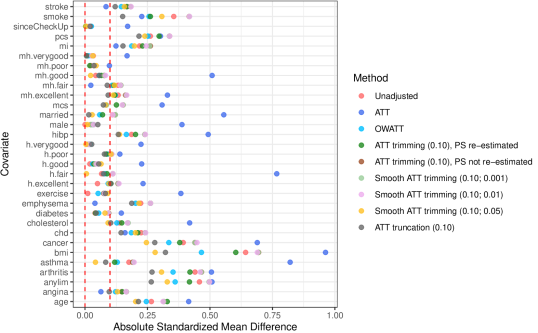
-
•
*The two red vertical dashed lines indicate the absolute difference within .
Table 3 shows 20 different WATTs, their points estimates and their estimated standard error (SE), using 500 bootstrap replicates. The OWATT has a point estimate of $2511.91 and ATT has $2399.32. Moreover, the point estimate of each ad-hoc method (trimming, smooth trimming, and truncation) increases as the threshold increases. The estimate from the trimming methods goes from less than $2500 to greater $3200, while those from truncation remain below $2500. For example, with ATT trimming where the PS is not re-estimated, the point estimates are, respectively, $2363.09, $2666.13, and $3054.09 for and , respectively. Similarly, for a fixed , the estimate of the smooth ATT trimming increases as decreases.
In terms of estimated bootstrap variances, the OWATT estimator has the smallest SE, except when compared against smooth ATT trimming for and . As expected, the ATT estimator has the largest SE due to the presence of extreme weights. For both trimming with and without re-estimating the PS, the higher the threshold , the lower the standard error. With smooth trimming, for a fixed , an increase in , results also in a decrease in SE, except when goes from to . For the same value of , the SE for truncation is better only when compared to ATT trimming without PS re-estimation. Otherwise, truncation is less efficient than ATT trimming with PS not re-estimated and smooth ATT trimming for the same threshold Overall, the OWATT estimator provides the best bias-variance trade-off and is better than truncation, both in teasing out the point estimate and by improving efficiency. Both trimming (smooth or not) and truncation give the impression that the more we trim or truncate, the better off we are. However, as demonstrated through our simulation studies, this can be misleading and may lead to a fishing expedition on where to stop in the choice of
| Method | Point estimate | Standard error | p-value |
| ATT | 2399.32 | 787.37 | 0.002 |
| OWATT | 2511.91 | 255.20 | |
| ATT trimming (), PS re-estimated | 2363.09 | 403.42 | |
| ATT trimming (), PS re-estimated | 2666.13 | 356.62 | |
| ATT trimming (), PS re-estimated | 3054.09 | 352.98 | |
| ATT trimming (), PS not re-estimated | 2487.25 | 352.16 | |
| ATT trimming (), PS not re-estimated | 2928.39 | 286.52 | |
| ATT trimming (), PS not re-estimated | 3286.90 | 270.04 | |
| Smooth ATT trimming () | 2488.98 | 348.88 | |
| Smooth ATT trimming () | 2926.52 | 285.92 | |
| Smooth ATT trimming () | 3291.05 | 268.68 | |
| Smooth ATT trimming () | 2419.59 | 327.68 | |
| Smooth ATT trimming () | 2881.88 | 277.57 | |
| Smooth ATT trimming () | 3229.41 | 259.47 | |
| Smooth ATT trimming () | 2337.55 | 373.65 | |
| Smooth ATT trimming () | 2638.19 | 250.78 | |
| Smooth ATT trimming () | 3014.23 | 232.06 | |
| ATT truncation () | 1945.35 | 385.00 | |
| ATT truncation () | 2211.56 | 307.63 | |
| ATT truncation () | 2419.23 | 271.39 |
6 Discussion
The positivity assumption is crucial to any propensity score (PS) method, but it is formulated differently depending on the estimand of interest and the method considered. For the average treatment effect on the treated (ATT), the postivity assumption requires that the PS of control participants be strictly less than 1. Violation (or near violations) of the positivity assumption leads to biased and even inefficient estimate of the ATT. Faced with this issue, the common practice is to target an ATT-like estimand by choosing an interval and either (1) trim i.e., exclude (smoothly or not) control participants whose PS falls outside the interval or (2) cap their weights to a fixed value (e.g., ), for a user-selected threshold . lee2011weight ; cole2008constructing
In this paper, we circumvented the subjectivity of selecting such a user-specified threshold (as well as the smooth parameter ) and considered instead a data-driven mechanism by multiplying the tilting function of the overlap weight to the conventional ATT weights of control participants. We have demonstrated that using such a tilting function has several advantages. First, it helps fulfill the positivity assumption, targets the population of control participants for whom there is a clinical equipoise,li2018balancing ; matsouaka2020framework and leads to efficient estimation. Second, the OWATT it helps characterize the treatment effect better when there is treatment effect heterogeneity. Indeed, using different thresholds (and possibly some smoothing parameters) for ATT trimming, smooth ATT trimming or ATT truncation can result in inconsistent pattern of treatment effect estimates when the effect is heterogeneous, as illustrated in our simulation and data analysis. On the other hand, OWATT uses available information from all participants, weighting each participant adequately based on their PS. Therefore, OWATT can potentially be a better alternative to ATT, under violations of positivity assumption—especially when such a violation is structural, i.e., due to inherent characteristics of the target population. petersen2012diagnosing ; westreich2010invited ; matsouaka2020framework
In addition, the proposed method is flexible and can be leveraged for any other appropriate functions for WATT estimand, which also helps define the target population . We plan to investigate in our future empirical studies the use of other , such as the Shannon’s entropy function or the matching function, that currently available in literature. zhou2020propensity ; li2013weighting ; matsouaka2020framework ; matsouaka2024overlap Moreover, our framework can be easily extended to the average treatment effect on the control (ATC), which is also considered in assessing the positive effect of interventions that aim to curb or end nefarious exposures. This can be, for example, an intervention for smoking cessation in a population of young adults or youth drug rehabilitation programs. Such an investigation has a considerable practical implication, especially when it comes to policy decision-making. matsouaka2023variance When there is a lack of positivity in estimating ATC, we suggest the use of to appropriately weight the treated participants and estimate the weighted ATC (WATC) as an alternative.
As shown in our simulation study, the methods presented in this paper are all biased when the PS model is misspecified, particularly the conventional ATT (without trimming and without truncation) weighting estimator which is the least robust against model misspecifications. Therefore, in practice, we suggest that a PS model as saturated as possible be postulated to gain higher accuracy of prediction. In that regard, one can use techniques such as penalized regression, series estimation, newey1994series or machine learning methods.lee2010improving ; li2021propensity In addition, we would like to mention that using machine learning methods may improve the PS estimation, and thus avoid the violation of positivity due to the misspecification of the parametric model. However, this does not help in the case where there is a structural violation of positivity assumption when the true PS distribution at the population level lacks positivity (as considered in our simulation in Section 4, too). petersen2012diagnosing A similar comment is about the use of another popular weighting method in causal inference, the calibration weighting (CW).imai2014covariate ; su2022sensitivity ; kott2016calibration CW used weights calculated based on some finite-sample moment equations, which also imposes covariate balance between the treatment groups. It can be viewed as another way to estimate the PS weights using some covariate balancing constraints, instead of the maximum likelihood estimation (MLE). However, when the violation of the positivity assumption is structural, the true covariate distributions between the treatment groups can be systematically different. Therefore, in this case, we suggest to “move the goalpost” to some subpopulation where the positivity is satisfied.crump2006moving In the context of ATT, the goalpost is a weighted or sub-population of the control participants. Our proposal of OWATT is a special case of such goalpost on controls, which can deal with both random and structural violations of positivity.
Finally, there are a number of important aspects of the WATT for which we leave a thorough investigation to future work. First, we have not investigated the semiparametric efficiency of the WATT estimators, abadie2005semiparametric ; crump2009dealing ; hirano2003efficient which can include additional modeling on outcomes and the study of corresponding augmented estimators. Furthermore, we can also leverage the M-theory, stefanski2002calculus ; tsiatis2007semiparametric and build sandwich-variance estimators lunceford2004stratification for the aforementioned weighting and augmented estimators and, ultimately, assess their robustness as well as their efficiency. Lastly, we have demonstrated in this paper that OWATT is a better alternative than the conventional ATT under lack of positivity. However, it is also worthy to investigate in theory and with great details how similar is OWATT to ATT when the overlap is good or moderate, which could potentially make the OWATT a more widely considered tool in more cases.
The authors are grateful to Dezhao Fu (Master of Biostatistics, Duke University) and Chenyin Gao (Department of Statistics, North Carolina State University), for helpful discussions in early stage of this research endeavor. We also thank Shi Cen (Bioinformatics Research Center, North Carolina State University) for his computational support. We especially thank the two anonymous reviewers and the editor for their patient and constructive feedback, which improved tremendously the quality of this paper.
References
- (1) Rosenbaum PR and Rubin DB. The central role of the propensity score in observational studies for causal effects. Biometrika 1983; 70(1): 41–55.
- (2) Busso M, DiNardo J and McCrary J. New evidence on the finite sample properties of propensity score reweighting and matching estimators. Review of Economics and Statistics 2014; 96(5): 885–897.
- (3) Ma X and Wang J. Robust inference using inverse probability weighting. Journal of the American Statistical Association 2020; 115(532): 1851–1860.
- (4) D’Amour A, Ding P, Feller A et al. Overlap in observational studies with high-dimensional covariates. Journal of Econometrics 2021; 221(2): 644–654.
- (5) Cole SR, Hernán MA, Robins JM et al. Effect of highly active antiretroviral therapy on time to acquired immunodeficiency syndrome or death using marginal structural models. American Journal of Epidemiology 2003; 158(7): 687–694.
- (6) Stürmer T, Rothman KJ and Glynn RJ. Insights into different results from different causal contrasts in the presence of effect-measure modification. Pharmacoepidemiology and drug safety 2006; 15(10): 698–709.
- (7) Kurth T, Walker AM, Glynn RJ et al. Results of multivariable logistic regression, propensity matching, propensity adjustment, and propensity-based weighting under conditions of nonuniform effect. American Journal of Epidemiology 2005; 163(3): 262–270.
- (8) Stürmer T, Rothman KJ, Avorn J et al. Treatment effects in the presence of unmeasured confounding: dealing with observations in the tails of the propensity score distribution—a simulation study. American journal of epidemiology 2010; 172(7): 843–854.
- (9) Crump R, Hotz VJ, Imbens G et al. Moving the goalposts: Addressing limited overlap in the estimation of average treatment effects by changing the estimand, 2006.
- (10) Dehejia RH and Wahba S. Causal effects in nonexperimental studies: Reevaluating the evaluation of training programs. Journal of the American statistical Association 1999; 94(448): 1053–1062.
- (11) Yang S and Ding P. Asymptotic inference of causal effects with observational studies trimmed by the estimated propensity scores. Biometrika 2018; 105(2): 487–493.
- (12) Crump RK, Hotz VJ, Imbens GW et al. Dealing with limited overlap in estimation of average treatment effects. Biometrika 2009; 96(1): 187–199.
- (13) Zhou Y, Matsouaka RA and Thomas L. Propensity score weighting under limited overlap and model misspecification. Statistical Methods in Medical Research 2020; 29(12): 3721–3756.
- (14) Ju C, Schwab J and van der Laan MJ. On adaptive propensity score truncation in causal inference. Statistical methods in medical research 2019; 28(6): 1741–1760.
- (15) Gruber S, Phillips RV, Lee H et al. Data-adaptive selection of the propensity score truncation level for inverse-probability–weighted and targeted maximum likelihood estimators of marginal point treatment effects. American Journal of Epidemiology 2022; 191(9): 1640–1651.
- (16) Li F, Morgan KL and Zaslavsky AM. Balancing covariates via propensity score weighting. Journal of the American Statistical Association 2018; 113(521): 390–400.
- (17) Hirano K, Imbens GW and Ridder G. Efficient estimation of average treatment effects using the estimated propensity score. Econometrica 2003; 71(4): 1161–1189.
- (18) Matsouaka RA and Zhou Y. A framework for causal inference in the presence of extreme inverse probability weights: the role of overlap weights. arXiv preprint arXiv:201101388 2020; .
- (19) Lawrance R, Degtyarev E, Griffiths P et al. What is an estimand & how does it relate to quantifying the effect of treatment on patient-reported quality of life outcomes in clinical trials? Journal of Patient-Reported Outcomes 2020; 4(1): 1–8.
- (20) Thomas LE, Li F and Pencina MJ. Overlap weighting: a propensity score method that mimics attributes of a randomized clinical trial. Jama 2020; 323(23): 2417–2418.
- (21) Li L and Greene T. A weighting analogue to pair matching in propensity score analysis. The international journal of biostatistics 2013; 9(2): 215–234.
- (22) Matsouaka RA, Liu Y and Zhou Y. Overlap, matching, or entropy weights: what are we weighting for? Communications in Statistics-Simulation and Computation 2024; 0(0): 1–20.
- (23) Mao H, Li L and Greene T. Propensity score weighting analysis and treatment effect discovery. Statistical Methods in Medical Research 2018; : 0962280218781171.
- (24) Greifer N and Stuart EA. Choosing the estimand when matching or weighting in observational studies. arXiv preprint arXiv:210610577 2021; .
- (25) Ben-Michael E and Keele L. Using balancing weights to target the treatment effect on the treated when overlap is poor. Epidemiology 2023; 34(5): 637–644.
- (26) Chattopadhyay A, Hase CH and Zubizarreta JR. Balancing vs modeling approaches to weighting in practice. Statistics in Medicine 2020; 39(24): 3227–3254.
- (27) Neyman J. Sur les applications de la théorie des probabilités aux experiences agricoles: Essai des principes. Roczniki Nauk Rolniczych 1923; 10: 1–51.
- (28) Imbens GW and Rubin DB. Causal inference in statistics, social, and biomedical sciences. Cambridge University Press, 2015.
- (29) Abadie A. Semiparametric difference-in-differences estimators. The review of economic studies 2005; 72(1): 1–19.
- (30) Heckman JJ, Ichimura H and Todd P. Matching as an econometric evaluation estimator. The review of economic studies 1998; 65(2): 261–294.
- (31) Stuart EA. Matching methods for causal inference: A review and a look forward. Statistical science: a review journal of the Institute of Mathematical Statistics 2010; 25(1): 1.
- (32) Busso M, DiNardo J and McCrary J. Finite sample properties of semiparametric estimators of average treatment effects. forthcoming in the Journal of Business and Economic Statistics 2009; .
- (33) Matsouaka RA, Liu Y and Zhou Y. Variance estimation for the average treatment effects on the treated and on the controls. Statistical Methods in Medical Research 2023; 32(2): 389–403.
- (34) Heckman JJ, Ichimura H and Smith J. Characterizing selection bias using experimental data. Econometrica 1998; 66(5): 1017–1098.
- (35) Smith JA and Todd PE. Does matching overcome lalonde’s critique of nonexperimental estimators? Journal of econometrics 2005; 125(1-2): 305–353.
- (36) Austin PC. Bootstrap vs asymptotic variance estimation when using propensity score weighting with continuous and binary outcomes. Statistics in Medicine 2022; 41(22): 4426–4443.
- (37) Lee BK, Lessler J and Stuart EA. Weight trimming and propensity score weighting. PloS one 2011; 6(3): e18174.
- (38) Li F, Thomas LE and Li F. Addressing extreme propensity scores via the overlap weights. American journal of epidemiology 2019; 188(1): 250–257.
- (39) Rubin DB. The design versus the analysis of observational studies for causal effects: parallels with the design of randomized trials. Statistics in medicine 2007; 26(1): 20–36.
- (40) Rubin DB. For objective causal inference, design trumps analysis. The Annals of Applied Statistics 2008; 2(3): 808 – 840.
- (41) Shao J and Tu D. The jackknife and bootstrap. Springer Science & Business Media, 2012.
- (42) Li Y and Li L. Propensity score analysis methods with balancing constraints: A monte carlo study. Statistical Methods in Medical Research 2021; 30(4): 1119–1142.
- (43) Kang JD, Schafer JL et al. Demystifying double robustness: A comparison of alternative strategies for estimating a population mean from incomplete data. Statistical science 2007; 22(4): 523–539.
- (44) Li F. Using propensity scores for racial disparities analysis. Observational Studies 2023; 9(1): 59–68.
- (45) Austin PC and Stuart EA. Moving towards best practice when using inverse probability of treatment weighting (iptw) using the propensity score to estimate causal treatment effects in observational studies. Statistics in medicine 2015; 34(28): 3661–3679.
- (46) Cole SR and Hernán MA. Constructing inverse probability weights for marginal structural models. American journal of epidemiology 2008; 168(6): 656–664.
- (47) Petersen ML, Porter KE, Gruber S et al. Diagnosing and responding to violations in the positivity assumption. Statistical methods in medical research 2012; 21(1): 31–54.
- (48) Westreich D and Cole SR. Invited commentary: positivity in practice. American journal of epidemiology 2010; 171(6): 674–677.
- (49) Newey WK. Series estimation of regression functionals. Econometric Theory 1994; 10(1): 1–28.
- (50) Lee BK, Lessler J and Stuart EA. Improving propensity score weighting using machine learning. Statistics in medicine 2010; 29(3): 337–346.
- (51) Imai K and Ratkovic M. Covariate balancing propensity score. Journal of the Royal Statistical Society: Series B (Statistical Methodology) 2014; 76(1): 243–263.
- (52) Su L, Seaman SR and Yiu S. Sensitivity analysis for calibrated inverse probability-of-censoring weighted estimators under non-ignorable dropout. Statistical Methods in Medical Research 2022; 31(7): 1374–1391.
- (53) Kott PS. Calibration weighting in survey sampling. Wiley interdisciplinary reviews: Computational statistics 2016; 8(1): 39–53.
- (54) Stefanski LA and Boos DD. The calculus of m-estimation. The American Statistician 2002; 56(1): 29–38.
- (55) Tsiatis A. Semiparametric theory and missing data. Springer Science & Business Media, 2007.
- (56) Lunceford JK and Davidian M. Stratification and weighting via the propensity score in estimation of causal treatment effects: a comparative study. Statistics in medicine 2004; 23(19): 2937–2960.
- (57) Van der Vaart AW. Asymptotic statistics, volume 3. Cambridge university press, 2000.
- (58) Greifer N. Covariate balance tables and plots: a guide to the cobalt package. Accessed March 2020; 10: 2020.
Appendix A Appendix: Technical Proofs
A.1 Equivalent formulas for ATT
A.2 Proof of Theorem 1
Denote the maximum likelihood estimator (MLE) of in the propensity score (PS) model . Define and for given data ,
We assume that , as a function of , is continuous almost everywhere with respect to . By Taylor expansion, we have
where and
The third “” follows from , under regularity conditions. (van2000asymptotic, ) Thus, is asymptotically linear.
Moreover, let us denote
We can verify that where
Furthermore, define and By conditioning arguments, for , we have .
Moreover, for ,
and
Therefore, we have, . Specifically,
In addition, we express as follows.
Therefore,
| (A.2.1) | ||||
| (A.2.2) | ||||
where is (A.2.1), and is (A.2.2). Therefore,
Finally,
| (A.2.3) | ||||
| (A.2.4) | ||||
| (A.2.5) | ||||
| (A.2.6) | ||||
| (A.2.7) | ||||
where the sum of (A.2.3)–(A.2.5) is , and the sum of (A.2.6)–(A.2.7) is . Note that (A.2.6) , and because they are scalars. Thus the proof is completed.
A.3 Asymptotic behaviors under misspecified propensity score model
Consider an estimating equation for a parameter of interest, . We solve the equation and get as the estimator of with truth . Under regularity conditions, by Talyor expansion, we have
therefore, the asymptotic bias of estimating using is
Therefore, the asymptotic bias of is approximately
| (A.3.1) |
Denote the estimated PS by , which converges to some quantity such that . If we correctly specify the PS model, then , otherwise it may not be true. Let and , where (resp. ) is also by plugging-in (resp. ).
Now for , consider the following estimating equation,
with the parameter of interest is , and with , where is by solving the equation. Therefore, the asymptotic bias of , by (A.3.1), is approximately
where . Hence,
Appendix B Appendix: Complete Simulation Results
| Scenario | |||||
| DGP I | DGP II | ||||
| Estimand | Good overlap | Moderate overlap | Poor overlap | Smaller adjusted | Kang and Schafer |
| ATT | 23.750 | 18.312 | 15.960 | 15.868 | 20.000 |
| OWATT | 23.946 | 18.894 | 16.009 | 15.976 | 16.871 |
| ATT trimming () | 23.761 | 18.765 | 16.212 | 16.166 | 19.476 |
| ATT trimming () | 23.815 | 18.661 | 15.709 | 15.677 | 17.787 |
| ATT trimming () | 23.900 | 18.376 | 15.134 | 15.108 | 15.583 |
| Smooth ATT trimming () | 23.761 | 18.765 | 16.212 | 16.166 | 19.475 |
| Smooth ATT trimming () | 23.815 | 18.661 | 15.710 | 15.677 | 17.790 |
| Smooth ATT trimming () | 23.900 | 18.376 | 15.134 | 15.108 | 15.582 |
| Smooth ATT trimming () | 23.753 | 18.652 | 16.365 | 16.166 | 19.452 |
| Smooth ATT trimming () | 23.769 | 18.692 | 16.176 | 15.679 | 17.780 |
| Smooth ATT trimming () | 23.802 | 18.637 | 15.940 | 15.111 | 15.582 |
| Smooth ATT trimming () | 23.762 | 18.758 | 16.212 | 16.037 | 19.030 |
| Smooth ATT trimming () | 23.815 | 18.658 | 15.711 | 15.694 | 17.614 |
| Smooth ATT trimming () | 23.900 | 18.374 | 15.137 | 15.170 | 15.643 |
| ATT truncation () | 23.779 | 18.607 | 16.052 | 16.309 | 19.850 |
| ATT truncation () | 23.827 | 18.574 | 15.725 | 16.128 | 19.245 |
| ATT truncation () | 23.890 | 18.334 | 15.195 | 15.898 | 18.342 |
B.1 Complete simulation results by DGP I

| Method | ARBias% | RRMSE | RMSE | RE | CP% |
| PS model correctly specified | |||||
| ATT | 0.29 | 0.037 | 0.87 | 0.96 | 95.20 |
| OWATT | 0.22 | 0.035 | 0.83 | 0.95 | 95.70 |
| ATT trimming (), PS re-estimated | 0.31 | 0.037 | 0.87 | 0.96 | 95.40 |
| ATT trimming (), PS re-estimated | 0.27 | 0.037 | 0.87 | 0.96 | 95.40 |
| ATT trimming (), PS re-estimated | 0.21 | 0.037 | 0.87 | 0.96 | 95.40 |
| ATT trimming (), PS not re-estimated | 0.31 | 0.037 | 0.87 | 0.96 | 95.40 |
| ATT trimming (), PS not re-estimated | 0.31 | 0.037 | 0.88 | 0.96 | 95.50 |
| ATT trimming (), PS not re-estimated | 0.26 | 0.037 | 0.88 | 0.97 | 95.30 |
| Smooth ATT trimming () | 0.31 | 0.037 | 0.87 | 0.96 | 95.40 |
| Smooth ATT trimming () | 0.31 | 0.037 | 0.88 | 0.96 | 95.40 |
| Smooth ATT trimming () | 0.26 | 0.037 | 0.88 | 0.97 | 95.40 |
| Smooth ATT trimming () | 0.31 | 0.037 | 0.87 | 0.96 | 95.40 |
| Smooth ATT trimming () | 0.31 | 0.037 | 0.87 | 0.96 | 95.30 |
| Smooth ATT trimming () | 0.26 | 0.037 | 0.88 | 0.97 | 95.40 |
| Smooth ATT trimming () | 0.30 | 0.037 | 0.87 | 0.96 | 95.60 |
| Smooth ATT trimming () | 0.29 | 0.036 | 0.87 | 0.96 | 95.30 |
| Smooth ATT trimming () | 0.25 | 0.036 | 0.87 | 0.96 | 95.60 |
| ATT truncation () | 0.30 | 0.037 | 0.87 | 0.97 | 95.20 |
| ATT truncation () | 0.31 | 0.037 | 0.87 | 0.96 | 95.50 |
| ATT truncation () | 0.30 | 0.037 | 0.87 | 0.96 | 95.50 |
| PS model misspecified | |||||
| ATT | 2.52 | 0.051 | 1.20 | 0.99 | 92.60 |
| OWATT | 2.46 | 0.049 | 1.17 | 0.98 | 92.70 |
| ATT trimming (), PS re-estimated | 2.48 | 0.050 | 1.19 | 0.99 | 92.70 |
| ATT trimming (), PS re-estimated | 2.25 | 0.049 | 1.17 | 0.99 | 93.30 |
| ATT trimming (), PS re-estimated | 1.97 | 0.047 | 1.13 | 0.98 | 93.80 |
| ATT trimming (), PS not re-estimated | 2.48 | 0.050 | 1.19 | 0.99 | 92.70 |
| ATT trimming (), PS not re-estimated | 2.25 | 0.049 | 1.17 | 0.99 | 93.30 |
| ATT trimming (), PS not re-estimated | 1.95 | 0.047 | 1.13 | 0.98 | 93.90 |
| Smooth ATT trimming () | 2.48 | 0.050 | 1.19 | 0.99 | 92.70 |
| Smooth ATT trimming () | 2.25 | 0.049 | 1.17 | 0.99 | 93.30 |
| Smooth ATT trimming () | 1.95 | 0.047 | 1.13 | 0.98 | 93.90 |
| Smooth ATT trimming () | 2.47 | 0.050 | 1.19 | 0.99 | 92.70 |
| Smooth ATT trimming () | 2.25 | 0.049 | 1.17 | 0.99 | 93.30 |
| Smooth ATT trimming () | 1.95 | 0.047 | 1.13 | 0.98 | 93.70 |
| Smooth ATT trimming () | 2.41 | 0.050 | 1.18 | 0.99 | 92.90 |
| Smooth ATT trimming () | 2.23 | 0.049 | 1.16 | 0.98 | 93.40 |
| Smooth ATT trimming () | 2.06 | 0.048 | 1.14 | 0.98 | 93.80 |
| ATT truncation () | 2.51 | 0.050 | 1.20 | 0.99 | 92.60 |
| ATT truncation () | 2.44 | 0.050 | 1.19 | 0.99 | 92.70 |
| ATT truncation () | 2.31 | 0.049 | 1.17 | 0.99 | 93.00 |
-
•
ATT: average treatment effect on the treated; OWATT: overlap weighted average treatment effect on the treated; PS: propensity score; ARBias%: absolute relative percent bias; RRMSE: relative root mean square error; RMSE: root mean square error; RE: relative efficiency; CP%: coverage probability (%).
| Method | ARBias% | RRMSE | RMSE | RE | CP% |
| PS model correctly specified | |||||
| ATT | 0.50 | 0.056 | 1.02 | 1.18 | 94.40 |
| OWATT | 0.15 | 0.039 | 0.73 | 0.99 | 94.80 |
| ATT trimming (), PS re-estimated | 0.02 | 0.040 | 0.75 | 0.98 | 95.20 |
| ATT trimming (), PS re-estimated | 0.55 | 0.041 | 0.76 | 1.00 | 95.00 |
| ATT trimming (), PS re-estimated | 1.39 | 0.043 | 0.79 | 0.99 | 94.20 |
| ATT trimming (), PS not re-estimated | 0.16 | 0.040 | 0.75 | 0.98 | 95.00 |
| ATT trimming (), PS not re-estimated | 0.19 | 0.040 | 0.74 | 1.00 | 94.90 |
| ATT trimming (), PS not re-estimated | 0.18 | 0.040 | 0.74 | 0.99 | 94.20 |
| Smooth ATT trimming () | 0.16 | 0.040 | 0.75 | 0.98 | 95.00 |
| Smooth ATT trimming () | 0.19 | 0.040 | 0.74 | 1.00 | 94.80 |
| Smooth ATT trimming () | 0.18 | 0.040 | 0.74 | 0.99 | 94.20 |
| Smooth ATT trimming () | 0.16 | 0.040 | 0.75 | 0.99 | 94.90 |
| Smooth ATT trimming () | 0.18 | 0.040 | 0.74 | 1.00 | 94.70 |
| Smooth ATT trimming () | 0.18 | 0.040 | 0.74 | 1.00 | 94.30 |
| Smooth ATT trimming () | 0.06 | 0.041 | 0.76 | 0.98 | 95.40 |
| Smooth ATT trimming () | 0.15 | 0.040 | 0.74 | 0.99 | 94.60 |
| Smooth ATT trimming () | 0.18 | 0.040 | 0.73 | 1.00 | 94.50 |
| ATT truncation () | 0.10 | 0.041 | 0.77 | 1.00 | 95.20 |
| ATT truncation () | 0.14 | 0.040 | 0.75 | 1.00 | 95.10 |
| ATT truncation () | 0.15 | 0.040 | 0.74 | 1.00 | 95.00 |
| PS model misspecified | |||||
| ATT | 3.93 | 0.074 | 1.35 | 1.16 | 83.40 |
| OWATT | 4.23 | 0.061 | 1.16 | 1.01 | 85.30 |
| ATT trimming (), PS re-estimated | 3.88 | 0.059 | 1.11 | 1.00 | 86.60 |
| ATT trimming (), PS re-estimated | 5.37 | 0.069 | 1.29 | 1.00 | 78.80 |
| ATT trimming (), PS re-estimated | 6.90 | 0.082 | 1.51 | 1.00 | 66.80 |
| ATT trimming (), PS not re-estimated | 3.53 | 0.057 | 1.07 | 1.00 | 88.50 |
| ATT trimming (), PS not re-estimated | 3.94 | 0.059 | 1.11 | 1.00 | 86.70 |
| ATT trimming (), PS not re-estimated | 4.03 | 0.061 | 1.12 | 1.00 | 86.60 |
| Smooth ATT trimming () | 3.53 | 0.057 | 1.07 | 1.00 | 88.50 |
| Smooth ATT trimming () | 3.94 | 0.059 | 1.11 | 1.00 | 86.80 |
| Smooth ATT trimming () | 4.03 | 0.061 | 1.12 | 1.00 | 86.70 |
| Smooth ATT trimming () | 3.52 | 0.057 | 1.07 | 1.01 | 88.60 |
| Smooth ATT trimming () | 3.93 | 0.059 | 1.11 | 1.00 | 86.70 |
| Smooth ATT trimming () | 4.03 | 0.061 | 1.12 | 1.00 | 86.60 |
| Smooth ATT trimming () | 3.63 | 0.059 | 1.11 | 1.03 | 87.40 |
| Smooth ATT trimming () | 3.82 | 0.059 | 1.10 | 1.01 | 87.20 |
| Smooth ATT trimming () | 4.01 | 0.061 | 1.11 | 1.00 | 86.80 |
| ATT truncation () | 3.22 | 0.058 | 1.07 | 1.03 | 88.90 |
| ATT truncation () | 3.50 | 0.058 | 1.08 | 1.02 | 87.70 |
| ATT truncation () | 3.67 | 0.058 | 1.08 | 1.01 | 87.40 |
-
•
ATT: average treatment effect on the treated; OWATT: overlap weighted average treatment effect on the treated; PS: propensity score; ARBias%: absolute relative percent bias; RRMSE: relative root mean square error; RMSE: root mean square error; RE: relative efficiency; CP%: coverage probability (%).
| Method | ARBias% | RRMSE | RMSE | RE | CP% |
| PS model correctly specified | |||||
| ATT | 1.64 | 0.074 | 1.19 | 1.51 | 91.20 |
| OWATT | 0.13 | 0.041 | 0.66 | 0.98 | 94.40 |
| ATT trimming (), PS re-estimated | 0.68 | 0.043 | 0.70 | 0.97 | 94.90 |
| ATT trimming (), PS re-estimated | 1.67 | 0.047 | 0.73 | 0.95 | 94.50 |
| ATT trimming (), PS re-estimated | 2.81 | 0.054 | 0.82 | 0.96 | 91.20 |
| ATT trimming (), PS not re-estimated | 0.08 | 0.042 | 0.68 | 0.97 | 94.80 |
| ATT trimming (), PS not re-estimated | 0.18 | 0.043 | 0.68 | 0.95 | 94.90 |
| ATT trimming (), PS not re-estimated | 0.21 | 0.046 | 0.69 | 0.99 | 94.10 |
| Smooth ATT trimming () | 0.09 | 0.042 | 0.68 | 0.97 | 95.00 |
| Smooth ATT trimming () | 0.18 | 0.043 | 0.68 | 0.96 | 94.90 |
| Smooth ATT trimming () | 0.21 | 0.046 | 0.69 | 0.99 | 94.20 |
| Smooth ATT trimming () | 0.10 | 0.042 | 0.68 | 0.98 | 94.90 |
| Smooth ATT trimming () | 0.18 | 0.043 | 0.68 | 0.97 | 94.70 |
| Smooth ATT trimming () | 0.20 | 0.045 | 0.69 | 0.99 | 94.40 |
| Smooth ATT trimming () | 0.13 | 0.046 | 0.74 | 1.05 | 94.70 |
| Smooth ATT trimming () | 0.11 | 0.042 | 0.66 | 0.98 | 94.40 |
| Smooth ATT trimming () | 0.17 | 0.044 | 0.66 | 0.98 | 94.20 |
| ATT truncation () | 0.11 | 0.043 | 0.70 | 1.00 | 94.30 |
| ATT truncation () | 0.12 | 0.042 | 0.68 | 0.99 | 94.20 |
| ATT truncation () | 0.13 | 0.042 | 0.67 | 0.99 | 93.90 |
| PS model misspecified | |||||
| ATT | 2.32 | 0.184 | 2.93 | 2.42 | 69.20 |
| OWATT | 5.91 | 0.075 | 1.20 | 1.00 | 76.80 |
| ATT trimming (), PS re-estimated | 6.60 | 0.080 | 1.30 | 0.99 | 70.80 |
| ATT trimming (), PS re-estimated | 7.78 | 0.090 | 1.42 | 0.98 | 62.80 |
| ATT trimming (), PS re-estimated | 9.45 | 0.106 | 1.60 | 0.99 | 49.90 |
| ATT trimming (), PS not re-estimated | 4.80 | 0.066 | 1.07 | 0.98 | 84.30 |
| ATT trimming (), PS not re-estimated | 4.56 | 0.065 | 1.02 | 0.97 | 86.10 |
| ATT trimming (), PS not re-estimated | 4.95 | 0.069 | 1.05 | 0.98 | 84.10 |
| Smooth ATT trimming () | 4.80 | 0.066 | 1.07 | 0.99 | 84.10 |
| Smooth ATT trimming () | 4.55 | 0.065 | 1.02 | 0.97 | 86.10 |
| Smooth ATT trimming () | 4.95 | 0.069 | 1.05 | 0.98 | 84.10 |
| Smooth ATT trimming () | 4.84 | 0.066 | 1.07 | 0.99 | 83.30 |
| Smooth ATT trimming () | 4.57 | 0.065 | 1.02 | 0.97 | 85.80 |
| Smooth ATT trimming () | 4.97 | 0.069 | 1.05 | 0.98 | 83.90 |
| Smooth ATT trimming () | 3.67 | 0.098 | 1.58 | 1.62 | 80.60 |
| Smooth ATT trimming () | 4.63 | 0.069 | 1.08 | 1.04 | 82.80 |
| Smooth ATT trimming () | 5.11 | 0.070 | 1.06 | 0.99 | 83.20 |
| ATT truncation () | 5.09 | 0.069 | 1.14 | 1.02 | 80.70 |
| ATT truncation () | 4.95 | 0.067 | 1.09 | 1.01 | 82.30 |
| ATT truncation () | 4.96 | 0.067 | 1.07 | 1.00 | 82.80 |
-
•
ATT: average treatment effect on the treated; OWATT: overlap weighted average treatment effect on the treated; PS: propensity score; ARBias%: absolute relative percent bias; RRMSE: relative root mean square error; RMSE: root mean square error; RE: relative efficiency; CP%: coverage probability (%).
| Method | ARBias% | RRMSE | RMSE | RE | CP% |
| PS model correctly specified | |||||
| ATT | 2.47 | 0.128 | 2.03 | 1.91 | 93.20 |
| OWATT | 0.14 | 0.062 | 1.00 | 0.94 | 96.00 |
| ATT trimming (), PS re-estimated | 0.90 | 0.075 | 1.21 | 0.94 | 96.70 |
| ATT trimming (), PS re-estimated | 1.89 | 0.073 | 1.15 | 0.89 | 95.50 |
| ATT trimming (), PS re-estimated | 2.98 | 0.081 | 1.22 | 0.94 | 95.00 |
| ATT trimming (), PS not re-estimated | 0.13 | 0.071 | 1.15 | 0.93 | 96.40 |
| ATT trimming (), PS not re-estimated | 0.06 | 0.067 | 1.06 | 0.90 | 97.20 |
| ATT trimming (), PS not re-estimated | 0.03 | 0.069 | 1.05 | 0.94 | 95.60 |
| Smooth ATT trimming () | 0.14 | 0.071 | 1.14 | 0.92 | 96.40 |
| Smooth ATT trimming () | 0.05 | 0.067 | 1.06 | 0.90 | 97.30 |
| Smooth ATT trimming () | 0.04 | 0.069 | 1.05 | 0.94 | 95.60 |
| Smooth ATT trimming () | 0.15 | 0.069 | 1.12 | 0.93 | 96.40 |
| Smooth ATT trimming () | 0.08 | 0.066 | 1.03 | 0.90 | 97.00 |
| Smooth ATT trimming () | 0.03 | 0.068 | 1.03 | 0.94 | 95.70 |
| Smooth ATT trimming () | 0.36 | 0.072 | 1.15 | 1.01 | 96.40 |
| Smooth ATT trimming () | 0.15 | 0.064 | 1.00 | 0.92 | 96.70 |
| Smooth ATT trimming () | 0.04 | 0.064 | 0.98 | 0.94 | 95.50 |
| ATT truncation () | 0.34 | 0.074 | 1.21 | 0.98 | 96.20 |
| ATT truncation () | 0.23 | 0.067 | 1.08 | 0.93 | 96.90 |
| ATT truncation () | 0.20 | 0.065 | 1.03 | 0.92 | 96.50 |
| PS model misspecified | |||||
| ATT | 3.45 | 0.198 | 3.14 | 3.68 | 85.80 |
| OWATT | 4.71 | 0.080 | 1.27 | 0.94 | 90.00 |
| ATT trimming (), PS re-estimated | 5.41 | 0.092 | 1.49 | 0.91 | 91.30 |
| ATT trimming (), PS re-estimated | 7.01 | 0.102 | 1.60 | 0.95 | 85.40 |
| ATT trimming (), PS re-estimated | 8.89 | 0.117 | 1.76 | 0.94 | 80.40 |
| ATT trimming (), PS not re-estimated | 3.91 | 0.082 | 1.32 | 0.91 | 93.30 |
| ATT trimming (), PS not re-estimated | 4.08 | 0.082 | 1.28 | 0.95 | 91.90 |
| ATT trimming (), PS not re-estimated | 4.58 | 0.085 | 1.28 | 0.96 | 90.70 |
| Smooth ATT trimming () | 3.91 | 0.081 | 1.32 | 0.91 | 93.50 |
| Smooth ATT trimming () | 4.09 | 0.081 | 1.28 | 0.95 | 91.90 |
| Smooth ATT trimming () | 4.58 | 0.085 | 1.28 | 0.96 | 90.90 |
| Smooth ATT trimming () | 3.97 | 0.080 | 1.30 | 0.92 | 93.30 |
| Smooth ATT trimming () | 4.06 | 0.080 | 1.26 | 0.95 | 91.50 |
| Smooth ATT trimming () | 4.55 | 0.083 | 1.26 | 0.95 | 90.70 |
| Smooth ATT trimming () | 3.35 | 0.100 | 1.61 | 1.56 | 90.80 |
| Smooth ATT trimming () | 4.09 | 0.079 | 1.24 | 0.98 | 92.00 |
| Smooth ATT trimming () | 4.60 | 0.081 | 1.23 | 0.95 | 89.90 |
| ATT truncation () | 4.00 | 0.087 | 1.41 | 0.98 | 92.20 |
| ATT truncation () | 4.04 | 0.080 | 1.29 | 0.95 | 91.80 |
| ATT truncation () | 4.17 | 0.079 | 1.25 | 0.95 | 91.90 |
-
•
ATT: average treatment effect on the treated; OWATT: overlap weighted average treatment effect on the treated; PS: propensity score; ARBias%: absolute relative percent bias; RRMSE: relative root mean square error; RMSE: root mean square error; RE: relative efficiency; CP%: coverage probability (%).

B.2 Complete simulation results by DGP II

| Method | ARBias% | RRMSE | RMSE | RE | CP% |
| PS model correctly specified | |||||
| ATT | 2.54 | 0.243 | 4.85 | 0.99 | 91.80 |
| OWATT | 1.56 | 0.170 | 2.86 | 0.90 | 95.70 |
| ATT trimming (), PS re-estimated | 1.99 | 0.226 | 4.40 | 0.97 | 93.20 |
| ATT trimming (), PS re-estimated | 0.88 | 0.220 | 3.91 | 0.87 | 96.40 |
| ATT trimming (), PS re-estimated | 3.10 | 0.240 | 3.74 | 0.81 | 95.90 |
| ATT trimming (), PS not re-estimated | 2.47 | 0.224 | 4.36 | 0.92 | 93.50 |
| ATT trimming (), PS not re-estimated | 3.77 | 0.226 | 4.02 | 0.83 | 96.50 |
| ATT trimming (), PS not re-estimated | 4.05 | 0.249 | 3.87 | 0.77 | 96.40 |
| Smooth ATT trimming () | 2.48 | 0.223 | 4.34 | 0.93 | 93.40 |
| Smooth ATT trimming () | 3.72 | 0.225 | 3.99 | 0.83 | 96.70 |
| Smooth ATT trimming () | 4.00 | 0.248 | 3.86 | 0.78 | 96.50 |
| Smooth ATT trimming () | 2.46 | 0.217 | 4.22 | 0.98 | 93.00 |
| Smooth ATT trimming () | 3.54 | 0.215 | 3.81 | 0.84 | 96.20 |
| Smooth ATT trimming () | 3.88 | 0.240 | 3.73 | 0.79 | 96.40 |
| Smooth ATT trimming () | 2.32 | 0.203 | 3.86 | 1.02 | 93.40 |
| Smooth ATT trimming () | 2.65 | 0.187 | 3.30 | 0.94 | 96.00 |
| Smooth ATT trimming () | 3.17 | 0.205 | 3.20 | 0.84 | 94.80 |
| ATT truncation () | 2.41 | 0.232 | 4.60 | 1.08 | 91.60 |
| ATT truncation () | 2.41 | 0.207 | 3.97 | 1.04 | 92.90 |
| ATT truncation () | 2.46 | 0.191 | 3.50 | 0.99 | 94.60 |
| PS model misspecified | |||||
| ATT | 36.72 | 0.420 | 8.39 | 0.91 | 50.80 |
| OWATT | 26.42 | 0.333 | 5.61 | 0.93 | 76.30 |
| ATT trimming (), PS re-estimated | 35.29 | 0.408 | 7.94 | 0.95 | 55.80 |
| ATT trimming (), PS re-estimated | 30.53 | 0.372 | 6.61 | 0.88 | 69.70 |
| ATT trimming (), PS re-estimated | 24.22 | 0.341 | 5.30 | 0.83 | 85.90 |
| ATT trimming (), PS not re-estimated | 35.26 | 0.408 | 7.93 | 0.96 | 55.70 |
| ATT trimming (), PS not re-estimated | 30.53 | 0.370 | 6.58 | 0.88 | 69.50 |
| ATT trimming (), PS not re-estimated | 24.21 | 0.337 | 5.25 | 0.84 | 85.20 |
| Smooth ATT trimming () | 35.25 | 0.407 | 7.92 | 0.96 | 55.80 |
| Smooth ATT trimming () | 30.51 | 0.370 | 6.57 | 0.88 | 69.40 |
| Smooth ATT trimming () | 24.20 | 0.337 | 5.24 | 0.84 | 84.90 |
| Smooth ATT trimming () | 35.13 | 0.405 | 7.88 | 0.97 | 55.40 |
| Smooth ATT trimming () | 30.55 | 0.370 | 6.56 | 0.90 | 68.70 |
| Smooth ATT trimming () | 24.12 | 0.334 | 5.20 | 0.85 | 84.40 |
| Smooth ATT trimming () | 34.16 | 0.396 | 7.53 | 0.98 | 57.70 |
| Smooth ATT trimming () | 30.38 | 0.366 | 6.44 | 0.95 | 67.50 |
| Smooth ATT trimming () | 24.60 | 0.330 | 5.16 | 0.90 | 82.70 |
| ATT truncation () | 36.24 | 0.415 | 8.24 | 0.98 | 51.80 |
| ATT truncation () | 34.63 | 0.400 | 7.70 | 0.98 | 56.40 |
| ATT truncation () | 32.33 | 0.381 | 6.98 | 0.97 | 62.10 |
-
•
ATT: average treatment effect on the treated; OWATT: overlap weighted average treatment effect on the treated; PS: propensity score; ARBias%: absolute relative percent bias; RRMSE: relative root mean square error; RMSE: root mean square error; RE: relative efficiency; CP%: coverage probability (%).
| Method | ARBias% | RRMSE | RMSE | RE | CP% |
| PS model correctly specified | |||||
| ATT | 0.12 | 0.125 | 2.50 | 1.10 | 92.80 |
| OWATT | 0.31 | 0.073 | 1.22 | 0.92 | 95.30 |
| ATT trimming (), PS re-estimated | 0.31 | 0.093 | 1.80 | 0.84 | 94.10 |
| ATT trimming (), PS re-estimated | 1.67 | 0.092 | 1.64 | 0.87 | 95.20 |
| ATT trimming (), PS re-estimated | 6.30 | 0.117 | 1.82 | 0.84 | 91.40 |
| ATT trimming (), PS not re-estimated | 0.76 | 0.093 | 1.81 | 0.81 | 94.20 |
| ATT trimming (), PS not re-estimated | 1.00 | 0.094 | 1.68 | 0.85 | 95.70 |
| ATT trimming (), PS not re-estimated | 0.57 | 0.105 | 1.63 | 0.81 | 96.50 |
| Smooth ATT trimming () | 0.77 | 0.092 | 1.80 | 0.82 | 94.10 |
| Smooth ATT trimming () | 0.97 | 0.094 | 1.66 | 0.85 | 95.60 |
| Smooth ATT trimming () | 0.60 | 0.104 | 1.62 | 0.82 | 96.30 |
| Smooth ATT trimming () | 0.59 | 0.089 | 1.73 | 0.86 | 94.10 |
| Smooth ATT trimming () | 0.91 | 0.090 | 1.59 | 0.88 | 95.00 |
| Smooth ATT trimming () | 0.67 | 0.101 | 1.57 | 0.84 | 95.80 |
| Smooth ATT trimming () | 0.31 | 0.085 | 1.62 | 0.94 | 94.20 |
| Smooth ATT trimming () | 0.57 | 0.077 | 1.36 | 0.90 | 95.60 |
| Smooth ATT trimming () | 0.64 | 0.088 | 1.37 | 0.91 | 95.60 |
| ATT truncation () | 0.18 | 0.102 | 2.02 | 0.98 | 93.30 |
| ATT truncation () | 0.42 | 0.086 | 1.65 | 0.92 | 94.30 |
| ATT truncation () | 0.48 | 0.078 | 1.43 | 0.90 | 95.10 |
| PS model misspecified | |||||
| ATT | 35.63 | 0.366 | 7.32 | 0.92 | 3.40 |
| OWATT | 24.83 | 0.263 | 4.43 | 0.90 | 20.10 |
| ATT trimming (), PS re-estimated | 34.09 | 0.351 | 6.84 | 0.91 | 3.90 |
| ATT trimming (), PS re-estimated | 28.90 | 0.303 | 5.37 | 0.87 | 13.60 |
| ATT trimming (), PS re-estimated | 21.73 | 0.240 | 3.73 | 0.86 | 49.40 |
| ATT trimming (), PS not re-estimated | 34.09 | 0.351 | 6.84 | 0.90 | 3.80 |
| ATT trimming (), PS not re-estimated | 28.90 | 0.302 | 5.37 | 0.86 | 12.80 |
| ATT trimming (), PS not re-estimated | 21.55 | 0.237 | 3.69 | 0.84 | 48.40 |
| Smooth ATT trimming () | 34.10 | 0.351 | 6.84 | 0.91 | 3.90 |
| Smooth ATT trimming () | 28.90 | 0.302 | 5.37 | 0.86 | 12.50 |
| Smooth ATT trimming () | 21.55 | 0.237 | 3.69 | 0.85 | 48.20 |
| Smooth ATT trimming () | 34.00 | 0.350 | 6.81 | 0.91 | 3.60 |
| Smooth ATT trimming () | 28.91 | 0.302 | 5.36 | 0.88 | 11.50 |
| Smooth ATT trimming () | 21.66 | 0.238 | 3.70 | 0.87 | 46.40 |
| Smooth ATT trimming () | 32.90 | 0.340 | 6.46 | 0.92 | 3.40 |
| Smooth ATT trimming () | 28.79 | 0.301 | 5.29 | 0.90 | 10.40 |
| Smooth ATT trimming () | 22.55 | 0.244 | 3.82 | 0.89 | 36.90 |
| ATT truncation () | 35.17 | 0.362 | 7.18 | 0.93 | 3.00 |
| ATT truncation () | 33.41 | 0.345 | 6.63 | 0.92 | 3.60 |
| ATT truncation () | 30.87 | 0.320 | 5.87 | 0.91 | 6.20 |
-
•
ATT: average treatment effect on the treated; OWATT: overlap weighted average treatment effect on the treated; PS: propensity score; ARBias%: absolute relative percent bias; RRMSE: relative root mean square error; RMSE: root mean square error; RE: relative efficiency; CP%: coverage probability (%).
Appendix C Appendix: Additional Data Analysis Results
In this section, we show an additional detail of the MEPS data analysis in Section 5. The following love plot in Figure C.0.1 displays the absolute standardized mean differences (ASD) (greifer2020covariate, ; austin2015moving, ) of 31 covariates between White and Asian group using weights in all 20 methods we considered in both simulation and data analysis. We use different shapes of points to indicate different thresholds we select within a given ad-hoc method.
As can be seen, ASDs by ATT weights exceed the threshold frequently and sometimes in a larger degree than other methods, and overall, OWATT, ATT trimming () with PS re-estimated, Smooth ATT trimming (), Smooth ATT trimming (), Smooth ATT trimming (), Smooth ATT trimming (), ATT truncation (), ATT truncation () balance covariates better than other methods.

-
•
The two red vertical dashed lines indicate the absolute difference within .