Average Spectral Density of Multiparametric Gaussian Ensembles of Complex Matrices
Abstract
A statistical description of part of a many body system often requires a non-Hermitian random matrix ensemble with nature and strength of randomness sensitive to underlying system conditions. For the ensemble to be a good description of the system, the ensemble parameters must be determined from the system parameters. This in turn makes its necessary to analyze a wide range of multi-parametric ensembles with different kinds of matrix elements distributions. The spectral statistics of such ensembles is not only system-dependent but also non-ergodic as well as non-”stationary”.
A change in system conditions can cause a change in the ensemble parameters resulting an evolution of the ensemble density and it is not sufficient to know the statistics for a given set of system conditions. This motivates us to theoretically analyze a multiparametric evolution of the ensemble averaged spectral density of a multiparametric Gaussian ensemble on the complex plane. Our analysis reveals the existence of an evolutionary route common to the ensembles belonging to same global constraint class and thereby derives a complexity parameter dependent formulation of the spectral density for the non-equilibrium regime of the spectral statistics, away from Ginibre equilibrium limit.
I Introduction
The unavoidable contact with environmental or dissipative aspect of real physical systems makes it necessary to consider the physics of non-Hermitian generators of the dynamics. Indeed recent developments in a wide range of complex systems e.g. dissipative quantum systems berry ; r1 ; r2 ; r3 ; r4 ; r5 ; r6 ; r7 ; r8 ; r9 ; r10 ; r11 ; r12 ; r13 ; r14 ; r15 ; r16 ; r17 ; r20 ; r21 ; r22 ; r23 , neural network dynamics and biological growth problems sc ; ns ; kr1 ; ahn ; afm ,statistical mechanics of flux lines in superconductors with columnar disorder fte classical diffusion in random media cw have refocused the attention on random non-Hermitian operators and a search for the mathematical models for their statistical properties e. g. cw ; cb ; psnh ; ben1 ; ben0 ; ben2 ; most ; jk ; gnt ; ir1 ; ir2 ; fh1 ; fz ; fy1 ; fy2 ; gin ; fy3 ; nh ; prosen ; hkku ; tk ; bp ; gnv ; swhjy ; mcn ; nm . As the average behavior of many of the physical properties can be determined from the average spectral density of the operators, its theoretical formulation is very desirable and is the primary focus of present study.
In general, a real physical system under consideration is often complex. Enormous success of Hermitian random matrix ensembles in past with the Hermitian operators of complex systems haak ; meta ; fkpt5 ; brody ; apbe ; psrev ; gmw ; psall ; psall1 ; psco ; ptche ; apce ; psalt ; psacu ; psflat encourages us to seek non-Hermitian random matrix ensembles as the models for the non Hermitian operators. But, as in the Hermitian case, the manifestation of the complexity is in general system dependent and the choice of an appropriate ensemble representing the system requires a prior knowledge of the relations among ensemble and system parameters and imposes various matrix as well ensemble constraints psrev . This in turn requires an analysis of a wide range of system dependent random matrix ensembles, with matrix elements described by multi-parametric distributions which may also be correlated. The growing applications of such ensembles in complex systems has in past led to development of a number of theoretical tools e.g. orthogonal polynomial method fy1 ; fy2 ; fy3 ; gnv , Green’s function approach fh1 ; nh ; sc , cavity method mcn ; nm , nonlinear sigma model approach haak etc. The results obtained are however often based on system specific approximations used to simplify the analysis gin ; haak ; bp ; gnv ; tk ; mnr . This motivated one of us in psnh to seek a theoretical formulation where all system information manifest through a single function of all system parameters. The study psnh however did not pursue a detailed analysis of the formulation e.g analysis of the spectral density or its fluctuations. Our primary objective in the present work is to bridge this information gap by deriving a common mathematical formulation for the spectral density of a wide range of Gaussian ensembles of complex matrices with varying degree of sparsity.
The contact with the environment subjects a physical system to many perturbations often causing a variation of system parameters with time. With a non-Hermitian Hamiltonian basically describing the interaction between system and its environment, and the latter often being dynamic, the Hamiltonian matrix is expected to evolve in complex matrix space with time-varying system conditions. But as the Hamiltonian matrix can also be represented by an ensemble or complex matrices at each instant of time; a variation of ensemble parameters results in evolution of the ensemble density on the ensemble space. This give rise to a natural query whether it is possible to find a path in the ensemble space, the evolution along which can exactly be mapped to evolution on the complex matrix space. The existence of such a path implies that the system is appropriately represented by the same ensemble for all instants of time. Additionally while the evolution in matrix space is governed by many system parameters, all of them vary with time, thereby implying time as the ultimate independent variable. The evolution in ensemble space is however governed by many ensemble parameters. It is therefore desirable to seek a time-like single parametric evolution in ensemble space too. Such an evolution if possible would indicate existence of universality classes, different from that of Ginibre and among non Hermitian ensembles belonging to a wide range of parametric dependences. Relevant initial steps in this context were made in the study psnh ; the latter derived, by an exact theoretical route, a diffusion equation for the joint probability distribution function (jpdf) for the eigenvalues of a multi-parametric Gaussian ensemble of non-Hermitian matrices. While a random perturbation of the matrix elements of such an ensemble can subject them to diffusive dynamics at different parametric scales (given by ensemble parameters), the diffusion of the eigenvalues was shown to be governed by a single functional of all the ensemble parameters. As the latter are functions of the system parameters, the functional, referred as the complexity parameter, contains the relevant information about the system under consideration. The existence of such a formulation, verified by the detailed numerical analysis on many body as well as disordered systems, has already been shown in past for the Hermitian operators psco ; psalt ; psall ; psall1 ; ptche ; psacu . As mentioned above, while the basic formulation for the non-Hermitian cases was derived in psnh , its detailed analysis on the complex plane e.g. the statistical fluctuations of the radial and angular parts of the eigenvalues, as well as the desired numerical verification was not pursued earlier (mainly due to lack of interest in non-Hermitian operators in past) and has been missing so far. An intense interest in the domain recently as well as robustness and wider applicability of the formulation now makes it desirable to extend our analysis of psnh further. In the present study, we derive an explicit formulation of the ensemble averaged spectral density of the sparse complex random matrices as a function of the complexity parameter. Our approach is based on four crucial steps: (i) first considering the evolution of a multiparametric Gaussian ensemble of complex matrices in the ensemble space due to variation of ensemble parameters and described by a combination of first order parametric derivatives, (ii) showing that it can exactly be mimicked by a diffusion in the matrix space with a constant drift, (iii) the multiparametric evolution can be reduced to an evolution governed by a single function of all ensemble parameters (therefore referred as complexity parameter), (iv) solving evolution equation for the average density of states.
The paper is organized as follows. Section II introduces the complexity parametric formulation of the ensemble density and thereby that of the jpdf of the eigenvalues on the complex plane. While the latter was derived in psnh by a direct route, the derivation presented here is based on the ensemble density and is richer as it can be extended to derive the distribution of the eigenfunctions too. As previous studies of the non-Hermitian ensembles are often focussed on those with free of any parameters e.g. Ginibre ensemble haak , the available results correspond to ergodic limit of statistical fluctuations. The presence of many parameters usually makes the spectral statistics non-ergodic as well as non-”stationary”. As our analysis is focussed on multiparametric ensembles, it is necessary to first define the concept of non-ergodicity as well as non-”stationarity” in an ensemble; this is discussed in section III. Section IV presents a derivation of the diffusion equation for the ensemble averaged spectral density in polar coordinates and its solution. This is followed by the numerical analysis, in section VI, for three different multi-parametric Gaussian ensembles of non-Hermitian matrices. The choice of these ensembles is basically motivated from their applicability to real systems as well as from the already available results for the similar Hermitian ensembles that helps in the comparative studies of the spectral fluctuations under Hermitian and non-Hermitian constraint. We conclude in section VII with a brief discussion of our main results, insights and open issues for future. We also note that a given symbol with different number of subscripts has different meaning throughout the text (e.g. and are not same).
II Diffusion of the eigenvalues on the complex plane
Consider a complex system represented by a non-Hermitian matrix with known constraints only on the mean and variances of the matrix elements and their pair wise correlations. Based on the maximum entropy hypothesis (MEH), it can be described by an ensemble of complex matrices defined by a multiparametric Gaussian ensemble density with as the column vector consisting of all matrix elements and as the covariance matrix. However, for technical reasons described in next section, here we consider an equivalent but alternate form, namely, with
| (1) |
with , as a constant determined by the normalization condition , and as the sets of distribution parameters of various matrix elements. Here the subscript on a variable refers to one of its components i.e real () or imaginary () part, with as total number of the components. As the ensemble parameters can be arbitrarily chosen (including an infinite value for non-random entries), can represent a large class of non-Hermitian matrix ensembles e.g. varying degree of sparsity or bandedness. For example, even a simple choice of almost all and with can lead to three different universality classes of stationary ensembles namely, Ginibre (), GUE () and the ensemble of complex antisymmetric matrices or GASE () and many non-stationary ones intermediate between them for sc ; fy1 ; nh . Further with choice of as the functions of system parameters, can act as an appropriate model for a wide range of non-Hermitian complex systems psnh .
II.1 Evolution of the ensemble density
A change in system conditions can affect the matrix elements , resulting in evolution of in matrix space. But as ensemble parameters are functions of system parameters, they also vary, leading to an evolution of in ensemble space too. Here the matrix space is a dimensional space (consisting of real and imaginary components of the matrix elements, with each point in the space corresponds to a non-Hermitian matrix. The ensemble space is a dimensional space consisting of independent ensemble parameters with each point representing the state of the ensemble.
For the evolving ensemble to continue representing the system, it is desirable that the evolution of in matrix space is exactly mimicked by that in ensemble space. This motivates us to consider a first order variation of the ensemble parameters and over time and seek (i) what type of matrix space dynamics they correspond to, and, (ii) can it lead to an equilibrium ensemble with stationary correlations? More explicitly, we consider following combination of the first order parametric derivatives
| (2) |
with
| (3) |
Here is an arbitrary parameter that gives the freedom to choose the end point of the evolution. For brevity of notations, hereafter will be written just as .
With help of its Gaussian form, the multi-parametric evolution of can be described exactly in terms of a diffusion, with finite drift, in -matrix space,
| (4) |
with .
As eq.(4) is difficult to solve for generic parametric values, we seek a transformation from the set of parameters to another set , with , such that only varies under the evolution governed by the operator and rest of them i.e remain constant: or where with defined by the condition (discussed in appendix A). This implies
| (5) |
Clearly should satisfy the condition that
| (6) |
As discussed in appendix A, the above set of equations can be solved by standard method of characteristics. The solution for is
| (7) |
with as the constant of integration, and expressed as function of . Here the sign for is chosen so as to keep it increasing above the initial value (following standard diffusion equation approach where plays the role of time and is always positive).
We note that the form of in eq.(7) is obtained by assuming all . For , eq.(3) gives and the corresponding derivative do not contribute to eq.(2). Indeed, for the cases in which a specific parameter throughout the evolution (with arbitrary), the number of evolving parameters is less than .
For the case , the constants and are given by the relations and . Integration in eq.(7) further gives
| (8) |
with , , . Here the symbol indicates the summation over non-zero only.
Similarly solution of eq.(6) for leads to constants of integrations which can be determined by the initial conditions as well as global constraints on the dynamics. (As a similar approach for Hermitian operators has been discussed in a series of studies psall , and in psnh for non-Hermitian operators, the details of the derivation are not included in this work). To distinguish it from with , hereafter will be referred as .
As a simple example (also used in our numerics discussed in section V), here we consider the case with . The latter corresponds to and thereby . Following from eq.(7), we then have
| (9) |
and for with as arbitrary constants of integration. (This can also be seen directly from eq.(6): for , it reduces to the condition which on solving gives eq.(9) for ).
An important insight in eq.(5) can be gained by noting the similarity of its form with the standard Fokker Planck (FP) equation, describing the diffusive dynamics of ”particles” in ”time” in a harmonic external potential and subjected to white noise. As the standard FP formulation is based on consideration of positive time like variable, hereafter we will consider ; the latter is ensured by choosing the appropriate sign in eq.(8) or eq.(9). Similar to FP equation, approaches the steady state in the limit of eq.(5) or as . For example, a choice of almost all and with fulfills the condition for and can therefore lead to three different types of steady states, namely, Ginibre (), GUE () and GASE (). As expected, the solution of eq.(5) with its left side set to zero is consistent with already known distributions for Ginibre, GUE and GASE (also follows from eq.(1) on substitution of the above values of ). As mentioned previously, for a random matrix ensemble to represent a complex system, an appropriate choice of the ensemble parameters must take into account all system-specifics, thereby rendering them to be functions of the system parameters. This in turn makes as the functional of the latter and thereby a measure of the complexity of the system.
As mentioned below eq.(3), is an arbitrary parameter and can be set to unit value too. Nonetheless it is useful to retain in the formualtion for two reasons: (i) it gives the freedom to analyze the statistical behavior of the system in or limit (e.g. the dynamics in absence off the confining harmonic potential part or in reducing the role of diffusion relative to drift term), (ii) also plays the role of a spectral unit in numerical analysis (e.g. while analyzing the approach of different ensembles to Ginibre universality class).
We emphasize that the form of eq.(5) is based on the specific forms for and given in eq.(3). Indeed it is motivated by our search for a combination of the parametric derivatives that would lead to a Dyson Brownian dynamics model in non-Hermitian matrix space (introduced by Dyson for Hermitian case and discussed in detail e.g. in haak ; meta ), starting from an arbitrary initial condition and with a Ginibre ensemble as the equilibrium limit. The search is motivated in turn by a hope to connect and utilise already existing technical tools developed for Dyson Brownian ensembles of Hermitian matrices haak ; meta ; apbe ; psrev ; circ ; psall ; psall1 ; psco .
The above mentioned connection motivates a natural query as to what type of dynamics (eq.(1)) undergoes if subjected to an evolution governed by an arbitrary combinations of parametric derivatives? Alternatively, if we consider a Brownian dynamics model for a non-Gaussian ensemble (i.e the combination of matrix element derivatives in right side of eq.(5)), can it still be described by a combination of the first order or higher order parametric derivatives? Some insights in this context are discussed in previous studies on Hermitian matrix ensembles psalt ; psco . As discussed in section V of psalt , not all parametric combinations would lead to an evolution in the Hermitian matrix space with an equilibrium limit. Besides, as discussed in section II.C or II. D of psco , not all combinations seem to be easily reducible to a single parametric dependence of the evolution (although a detailed investigation is needed in this context).
II.2 Evolution of the jpdf of the eigenvalues
Contrary to a spectral degeneracy of a Hermitian matrix, a nonhermitian matrix is non-diagonalisable at the exceptional points i.e the points in the parameter space at which some of the eigenvalues become degenerate and the corresponding eigenvectors coalesce into one ir2 . But as the number of exceptional points is at most finite, the non-Hermitian matrices are considered to be diagonalisable. We hereafter refer the parametric conditions avoiding exceptional points as non-exceptional.
Assuming non-exceptional parametric conditions, a non-Hermitian matrix can be diagonalized by a transformation of the type with as the matrix of eigenvalues and and as the left and right eigenvector matrices respectively. Here we consider the case of complex matrices () only, with its eigenvalues , in general, distributed over an area in the complex plane and as unitary matrices; here subscript refers to the real or imaginary components of the eigenvalues). Let be the jpdf of the eigenvalues at arbitrary values of and with . An integration of eq.(5) over all eigenfunctions components leads to an evolution of with ; for symbols consistency with earlier works, hereafter will be referred as . Let be related to the normalized distribution by , its governed evolution can then be described as (details discussed in appendix B)
| (10) |
with and
| (11) |
As discussed in appendix B, the derivation of eq.(10) is based on the set of eq.(109) describing the response of the eigenvalues as well as the eigenvectors to a small change in the matrix element ; the assumption of as unitary matrices is necessary for these relations. As discussed in psnh , an assumption of only leads to different dynamics of eigenvalues and eigenfunctions with varying matrix elements; this in turn leads to a n evolution equation for different from eq.(10).
In the limit or , the evolution described by eq.(10) reaches the equilibrium steady state of the Ginibre ensemble with ; the steady state limit occurs for the system conditions resulting in almost all and with . Thus eq.(10) describes a cross-over from a given initial ensemble (with ) to Ginibre ensemble as the equilibrium limit with as the crossover parameter. The non-equilibrium states of the crossover, given by non-zero finite values of , are various ensembles of the complex matrices corresponding to varying values of ’s and ’s thus modelling different complex systems. A point worth emphasizing here is following: while the ”equilibrium” and ”non-equilibrium” states mentioned above occur on the ensemble space, such ensembles may well-represent complex systems in e.g. thermal non-equilibrium stages too.
III Local ergodicity and ”non-stationarity” of the spectrum
The spectral density at a point on the complex spectral plane is defined as
| (12) |
where with as complex conjugate of subjected to the normalization condition . Its average over an ensemble at a given point on the spectral plane can then be expressed as
| (13) |
with and as the ensemble average,
Under assumptions that is separable into two components, a slowly varying (the secular behavior), and a rapidly varying , it can be written as (describing the local random excitations of ). A spectral averaging over a scale larger than that of the fluctuations gives and . The removal of the slowly varying part by a rescaling then provides the information about local fluctuations. Referred as ”unfolding” of the spectrum, this is achieved by redefining the real and imaginary parts of the spectral variable : and of the eigenvalues which results in a uniform local mean spectral density psnh ; psgs2 .
III.1 Local ergodicity of the spectrum
Experimental results are often based on a single spectrum analysis; this leaves the unfolding by as the only option. But theoretical modelling of a single complex system by an ensemble of its replicas is often based on the assumptions of local ergodicity i.e the averages of its properties over a given spectral range, say around , for a single matrix (referred as the spectral average) are same as the averages over the ensemble at a fixed (referred as the ensemble average). Mathematically this implies
| (14) |
with implying an ensemble average for a fixed and thereby permits it to be used for a theoretical unfolding of the spectrum. Prior to application of theoretical results to experimental data, it is therefore necessary to check the ergodicity of the spectrum. (An important point worth emphasizing here is as follows. The concept of ergodicity, a standard assumption in conventional statistical mechanics, implies analogy of the phase space averaging (i.e averaging over an ensemble of micro states) of a measure with time averaging. In case of a random matrix ensemble, the phase space averages are replaced by the averages over an ensemble of matrices and time averages by the spectral averages; the ergodicity of a measure now implies the analogy of ensemble averaging with spectral averaging. )
The fluctuations in local spectral density can in principle be measured in terms of the order spectral density correlation , defined as psnh
| (15) |
with . The above definition is valid in general for an arbitrary non-Hermitian ensemble. As clear from a comparison with eq.(13), the case corresponds to the ensemble averaged spectral density and is subjected to following normalization condition: .
An ergodic level density does not by itself implies the ergodicity of the local density fluctuations. Here we generalise the definition for the non-Hermitian case: the ergodicity of a local property say ”” can be defined as follows: let be the distribution function of in the neighbourhood ”s” of an arbitrary region ”” over the ensemble and be the distribution function of over a single realisation, say ”” of the ensemble: is defined as ergodic if it satisfies the following conditions: (i) the distribution for almost each realization is same i.e is independent of for almost all , implying , (ii) the distribution over the ensemble is analogous to that of single realization , (iii) is stationary on the spectral plane i.e independent of : for arbitrary points on the complex plane, However if condition (iii) is not fulfilled, is then referred as locally ergodic. More clearly, an ensemble is locally ergodic in a spectral range say around , if the averages of its local properties over the range for a single matrix (referred as the spectral average) are same as the averages over the ensemble at a fixed (referred as the ensemble average). It is worth re-emphasizing here the relevance of the translational/ rotational invariance in the bulk of a spectrum: as clear from the above, it implies an invariance of the local fluctuation measures from one spectral point on the complex plane to another. A non-invariant spectrum can at best be locally ergodic and therefore a complete information about the spectrum requires its analysis at various spectral ranges.
III.2 Non-stationarity of the spectrum
A generic random matrix ensemble need not contain an explicit time dependence and it is necessary to first define ”stationarity” in this context. This refers to a dynamics of the ensemble, in ensemble space, due to variation of the ensemble parameters; this in turn leads to leads to variation of the statistical properties. The stationarity (equilibrium) limit here corresponds to the ensemble parameter values for which ensemble becomes invariant under a set of transformations related to global constraints. The intermediate states of the ensemble as its parameters vary from an arbitrary initial state to stationary limit, are then referred as ”non-stationary” or “non-equilibrium” ensembles.
As clear from the above, a non-stationarity of the spectrum in present context refers to its pseudo time-dependence. For example, as mentioned above, the solution of eq.(10) corresponds to stationary Ginibre ensemble in the equilibrium limit . The intermediate states of the evolution for finite are then referred as non-stationary ensembles. It is important to reemphasize the difference between non-ergodicity and non stationarity of the spectrum: the former refers to a non homogeneous statistics on the complex spectral plane at a fixed , the latter refers to change of statistics at a specific spectral point of interest with changing .
As discussed in previous section, the ensemble density (1) is both non-ergodic as well as non-stationary. In the next section, we analyze the dynamics of its spectral density in complex plane as varies.
IV Spectral Density on the complex plane: angular and radial dependence
As the definition (15) for indicates, the -dependence of manifests in too. The evolution equation for the latter can then be obtained by an integration of eq.(10) over all eigenvalues except one of them, say (hereafter, using notations and as the real and imaginary parts of ),
| (16) |
with indicating the principle part of the integral (details in appendix C).
A desirable next step would be to solve the above equation exactly but the presence of integral renders it technically difficult. With eigenvalues distributed on the complex plane, a deeper insight in the behavior can be gained by analyzing it in polar coordinates . Substitution of reduces eq.(16) as (details in appendix D)
| (17) |
where
| (18) | |||||
| (19) |
and
| (20) | |||||
| (21) |
Hereafter the integration limits will not be mentioned explicitely unless needed for clarity.
As the right side of eq.(17) is -independent, it can be solved by separation of variables approach. Considering a solution
| (22) |
with and , we have
| (23) |
with and again given by eq.(18) and eq.(19) respectively but with replaced by . Here for finiteness of as becomes large.
As both and are dependent on as well as , eq.(17) indicates a non-ergodic spectral density, correlated in and variables. Based on certain approximations specific to -range, these correlations can however be neglected, suggesting the separable solution
| (24) |
As the approximations are different for different -ranges, we now consider the behavior of in three different -regions and seek justification for the above conjecture, both analytically and theoretically.
IV.1 , bulk region:
By expanding eq.(20) and eq.(21) in powers of , we have and . Substitution of the above in eq.(18) and eq.(19) leads to
| (25) | |||||
| (26) |
with
| (29) |
As both and are -dependent, substitution of the above leaves eq.(23) non-separable in variables. In the regime , however, the series in eq.(29) can contribute significantly only if and vary as or faster.
The latter not only requires (such that ) but also its dependence on (to keep non-zero contributions from the integrals in eq.(29) for all ). But as is not very sensitive to angular dependence, this in turn suggests a -independence of near origin () and is also confirmed by our numerical analysis of three different ensembles, discussed later in section V. As a consequence, for almost all cases (e.g except for those with phase singularities at the origin psps ), the contribution of the series in eq.(29) to eq.(23) is negligible with respect to other terms and we can write
| (30) |
| (31) | |||||
| (32) |
Using separation of variables, the solution of above equations can be given as
| (33) | |||||
| (34) |
with as the Bessel’s functions, , as arbitrary constants, determined by the boundary conditions on ; the condition that latter remains finite at then implies . The single valuedness of as requires and with as integers and thereby . To keep as a real number, only allowed values of . The later in turn gives . Noting that , hereafter we use .
As the arbitrary constant is not subjected to any additional known constraints except semi-positive definite one, a valid particular solution can occur for continuous range of from . By substitution of the solutions in eq.(33) and eq.(34) for (equivalently ) in eq.(22), the general solution of eq.(17) for arbitrary initial condition (but finite at ) and for can now be given as
| (35) |
with constant determined by the initial condition of (examples discussed in appendix E). A circular symmetric behavior of is also confirmed by our numerics discussed in section V, thus lending credence to our separability conjecture in eq.(24).
The existence of a stationary solution in limit requires . The solution in the limit becomes
| (36) |
Here the condition,that remains finite requires ; this in turn gives a constant for .
We note that the solution in eq.(35) is obtained for smooth behavior of the density at . The solution for the cases in which initial spectral density is singular at , we must also consider .
IV.2 , edge region:
Expanding eq.(20) and eq.(21) in powers of , we have , . Substitution of the above in eq.(18) and eq.(19) leads to
| (37) | |||||
| (38) |
with
| (39) | |||||
| (40) |
with as a function of . Using the above, we have
| (41) |
Here but and , for , are complicated functions of .
Fortunately however the contribution from the terms containing , for can be neglected with respect to and (with ) for an asymptotic decay in decay. This can be explained as follows: in the regime , the series in eq.(41) can contribute significantly only if and vary as or faster. The latter in turn requires but this is not the case (as is dominated by the behavior near origin due to decreasing spectral density for large ). This is again confirmed by our numerical analysis of three different ensembles, discussed later in section V Assuming this to be the case, a substitution of the relation in eq.(17), retaining only term, now leads to
| (42) |
with .
As our interest here is in the cases with decaying spectral density away from the origin (i.e relatively lower spectral density in the edge region), the contribution to -integral in is dominated by the bulk, this implies is large (with respect to mean level spacing ) for the dominant part of the -integral. We can then safely assume . (This is based on rewriting in terms of the order cluster function haak ; circ ; meta : . But as is of order or lower) smaller than the other term, we can approximate . The latter approximation is the standard route used in past for Hermitian as well as unitary ensembles (discussed in detail in section(6.14) and specifically eq.(6.14.5) of haak , also discussed below eq.(59) in circ in case of circular Brownian ensembles). Using the above approximation we have with
| (43) |
Substitution of eq.(24) now leads to (with )
| (44) | |||||
| (45) |
with as an arbitrary constant, determined by the boundary conditions that vanishes at large radial distances and is single valued in . This in turn corresponds to following constraints: and . A particular solution of eq.(44) for an arbitrary constant is
| (46) |
with and , as the confluent Hypergeometric function temme , , and as arbitrary constants to be determined by the initial conditions. Noting that both appear along with , their influence on the solution can be seen only if they are of the order of or larger. We redefine them, without loss of generality (both constants being arbitrary), as and with as arbitrary constants to be determined by boundary conditions; the conditions that however also requires and . This lead to and thereby in large limit, and . The particular solution of eq.(44) can now be given as
| (47) | |||||
As the above solution is valid in large -limit, the first term with coefficient , for , is negligible as compared to second term. For , however, the first term approaches a constant value. The condition in eq.(46) therefore requires .
The solution of eq.(45) depends on the form of in eq.(43). Using , we can rewrite with and . For the case with ,we have . Eq.(45) then reduces to and its solution can be given as that of eq.(32)). For the case with , we have (with and ; the second order derivative in eq.(45) can then be neglected with respect to other terms. For , the solution of eq.(45) can now be given as,
| (48) |
with as an arbitrary constant and
| (49) |
| (50) |
By substitution of eq.(LABEL:umn), eq.(48) in eq.(24) and subsequently in eq.(22) for , the general solution for can now be given as
| (51) |
with arbitrary constants and determined from the initial solution (examples discussed in appendix E).
Here again for stationary solution to exist in limit , we need . This leads to, with given by eq.(47),
| (52) |
with . As the term is the dominant term in the above series, can further be approximated as
| (53) |
where we have used the identity temme .
IV.3 Arbitrary with rapidly decaying second order correlations:
With both as well as dependent on four variables , the determination of and from eq.(18) and eq.(19), for arbitrary , is technically complicated. Important insights in the solution can however be gained by a Taylor series expansion of and in the neighborhood of .
(i) Rapidly decaying angular moments of for arbitrary :
From eq.(20) and eq.(21), we note that at for as a positive integer and and at have a singularity at . can then be simplified by a Taylor series expansion of and as powers of in the neighborhood of . While this results in a series of double integrals over , the dominant contribution for each -integral comes from the region in neighborhood of , leading to
| (54) |
with
| (55) | |||||
| (56) |
where
| (57) |
and as the th moment of (equivalently that of jpdf of the eigenvalues) and is a function of variables and as well. Some lower orders of can be given as follows: , , , , , , , . Using the above, we have
| (58) |
While the main contribution to -integral in both and comes only from the neighborhood of (as both and have a pole there), the -integral is dominated by the region . For , this implies the correlation between two eigenvalues located at far-off points on the complex plane (although same radial distance but at an angle of ) and is expected to be negligible. As describes the second order spectral correlation at the scale of local spectral density , the correlation between such points is expected to be weak and we can approximate . This in turn gives with and thereby , . Further noting that and , it is reasonable to assume that become very small for , thereby making the contribution from and negligible relative to . This in turn permits eq.(58) to be approximated as follows: where . Substitution of the above approximations reduces eq.(17) to
| (59) |
Due to, , the above equation is still not separable in and variables and further progress can be made only by using case-specific forms of .
As an example, here consider the case with weak order density correlations all over the complex plane that permits ; (we note that the approximation is different from the one used above to calculate and , and is valid in general at distances larger than local mean level spacing). can then be expressed as
| (60) |
Multiplying eq.(17) by and substituting , we now have
| (61) | |||||
| (62) |
with , as an arbitrary constant, determined by the boundary conditions that vanishes at large radial distances and is single valued in . Further the first term in eq.(79) can be neglected, due to its being times smaller than the other terms. We note, following from eq.(60), the above equations are valid within the region on the complex plane where is non-zero.
The solution of eq.(61) depends on mathematical form of defined in eq.(60). As the correlations depend on system conditions, can in general be of different form as varies. Here we consider three representative cases. For the cases in which with as a constant, eq.(61) is of the same form as that of eq.(44), except for in the latter is now replaced by . The solution for can then be given by eq.(46) but now is replaced by and (as is finite in the present case). Proceeding again as in previous case, the solution now becomes (with )
| (63) | |||||
with arbitrary constants determined from initial condition at .
Similarly for the cases in which eq.(60) gives with as a constant, eq.(61) is again of the same form as that of eq.(44), except for in the latter is now replaced by and by a zero. Proceeding again as in previous case, the solution now becomes, with and ,
| (64) | |||||
with and as arbitrary constants.
Another case worth consideration is with . Eq.(61) is now approximately of the same form (by neglecting terms containing and with respect to constant terms and ) as that of eq.(44), except for in the latter is now replaced by a zero. Further, for technical simplification but without any loss of generality, we write as , with again a non-negative integer and as an arbitrarily small positive constant; the choice ensures arbitrariness of as well as permits its almost continuous values. (It is sufficient to choose for the present analysis). We now have
| (65) | |||||
Contrary to radial evolution, the angular evolution described by eq.(62) differs from eq.(45) and is similar to eq.(32); its solution can then be given by eq.(34); here again singlevaluedness of the solution requires but now where for the cases and ; for the case .
By substitution of appropriate along with eq.(34) in eq.(24) and subsequently in eq.(22) for , the general solution for can now be given as
| (66) |
where for and , for and the arbitrary constants in the above solution determined from the initial solution (examples discussed in appendix E). Here again a summation over transforms to -dependent function, leaving -dependent part independent of . The latter implies -dependence of does not vary significantly with . As discussed in section V, this is confirmed by our numerical analysis too which again supports our conjecture in eq.(24) (as the result in eq.(66) depends on the conjecture). Using eq.(66), in this case again corresponds to (equivalently ) and can be given as
| (67) |
Here again retaining only the dominant term corresponding to gives . From eq.(63) and eq.(64), we then have
| (68) | |||||
| (69) |
Here we have used and . The above indicates a constant density within the bulk spectral region for the case . Further the solution for case is of same form as in eq.(69) but with replaced by . We also note that, for a finite at in for the case or , we must have and .
We recall that the solutions (66) and (67) are applicable for the case with weak second order spectral correlations in the complex plane leading to or . We note that the solution for the last case remains valid for decalying faster than expoenential too. The solutions for other cases can be obtained by case specific approximation of eq.(59).
(ii) Slowly varying radial moments of around arbitrary :
For such cases, we can expand and in the neighborhood of . This leads to
| (71) |
Here the first term in the series is obtained by using and
| (72) |
with as the order moment of about a point and for a fixed and and defined as .
The integral in eq.(19) can similarly be approximated by Taylor series expansion of eq.(21); the latter gives
| (74) |
where
| (75) |
The series expansion of in eqs.(71, 74) are exact but their substitution in eq.(17) again leads to a differential equation non-separable in variable and not easy to solve. As clear from eq.(72) and eq.(75), the non-separability arises from the terms with and , , in the series. Fortunately however the contribution from to eq.(71) is negligible for the spectral distributions with slowly varying moments around point ; this is because that the dominant contribution from the integration over comes from the neighborhood of i.e equivalently . Assuming as a slowly varying function of , it can then be approximated by its value at . We then have
| (76) |
The above equality follows due to . Although, the -integration in case of is not dominated by the region around , we have . Thus if the moments are slowly varying functions of around arbitrary , the contribution from the higher order terms, i.e those with in eq.(71) and with in eq.(74)), can be neglected as compared to the first term. This in turn permits following approximations
| (77) |
Here the first term in is obtained by using the relation .
Substitution of the approximations (77) reduces eq.(17) separable in and variables. This can be seen as follows. Multiplying eq.(17) by and substituting , we now have
| (78) | |||||
| (79) |
with as an arbitrary constant, determined by the boundary conditions that vanishes at large radial distances and is single valued in . Further the first term in eq.(79) can be neglected, due to its being times smaller than the other terms.
As in previous case, here again eq.(78) is same as eq.(44) except for in the former and in the latter; the solution for can then again be given by eq.(46), using and finite. This again leads to eq.(63) but with and .
Contrary to radial evolution, the angular evolution described by eq.(79) differs from eq.(45) and is seemingly more complicated. Important insight in its solution can however be obtained by noting following analogy: substitution of the relation
Eq.(59) of circ however describes the evolution of the ensemble averaged spectral density of the circular Brownian ensembles of unitary matrices, with eigenvalues distributed on a unit circle) in terms of a perturbation parameter circ for arbitrary initial conditions; (note here too the second order derivative was neglected due to negligible contribution in large -limit) Its general solution is given as with permitted values of the constant given by the boundary conditions. The above implies that of our case corresponds to a particular solution of the average spectral density of the circular Brownian ensemble.
As for large , the evolution in circular ensemble case is known to approach uniform distribution with irrespective of the initial conditions. This in turn suggest . Further if the initial condition at is a uniform density e.g , the same behavior then persists for all ; this again implies . We note a uniform distribution of is also indicated by our numerics of three different Gaussian ensembles of complex matrices discussed in next section.
Substitution of eq.(63) in eq.(22) along with , the general solution for in the present case can be given as
| (81) |
with the arbitrary constants again determined from the initial solution . Again, with condition in limit, we have .
IV.4 Comparison with Ginibre ensemble:
As mentioned in section II, the evolution of the ensemble density (12) approaches, in the limit , an equilibrium steady state described by Ginibre ensemble; thus corresponding must also approach that of Ginibre ensemble in the above limit. A previous study haak (in section 8.8.2 therein) gives for finite ; It approches a uniform distribution within a radius in large limit: . It is instructive to compare the above result with limit of our results. From eqs.(36, 53, 67, LABEL:rinf4), we have within and decaying exponentially beyond the regime and is a constant in too. Thus our results are consistent with haak in large limit;
V Numerical analysis of spectral correlations
Our primary focus in this study is to numerically analyze following two aspects of the spectral density: (i) the non-ergodic as well as non stationary aspect i.e dependence on the energy range, (ii) the system dependence.
Our first objective has its roots in the immense interest generated by non-ergodic aspects of many body spectrum for Hermitian as well non-Hermitian operators; the ergodicity, or its absence, is characteristic of a system’s approach to thermalization which in turn facilitates the application of standard statistical tools. The motivation for the second objective comes from the unavoidable presence of disorder as well as many body interactions in physical systems which can manifests in a variety of ways in the matrix representation of their non-Hermitian operators; it is natural to query whether presence of disorder with/ without interactions has any, and if so, what impact on the average spectral density.
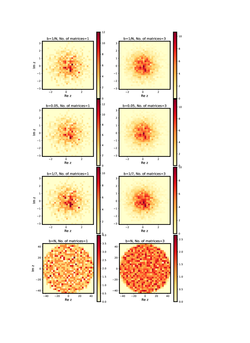
To achieve the objectives mentioned above, here we numerically analyze three ensembles of non-hermitian random matrices with independent, Gaussian distributed matrix elements with zero mean but different functional dependence of their variances. The ensemble density in each case is given by eq.(1), with for all and indices but varying among elements. The details of the latter for the three ensembles are as follows:
(i) Ensembles with same off-diagonal to diagonal variance for all matrix elements, referred here as Brownian ensemble (BE): . From eq.(9), this corresponds to (for a large ),
| (82) |
with as a constant. Choosing initial BE with then gives .
We recall that our theoretical formulation of the spectral density in section IV is based on standard assumption of (as mentioned below eq.(22). For comparison with our numerical analysis, it is therefore appropriate to ensure with increasing . For this reason, eq.(82) is obtained by choosing negative sign in eq.(9). The same reasoning will also be used for eq.(83) and eq.(84) given below.
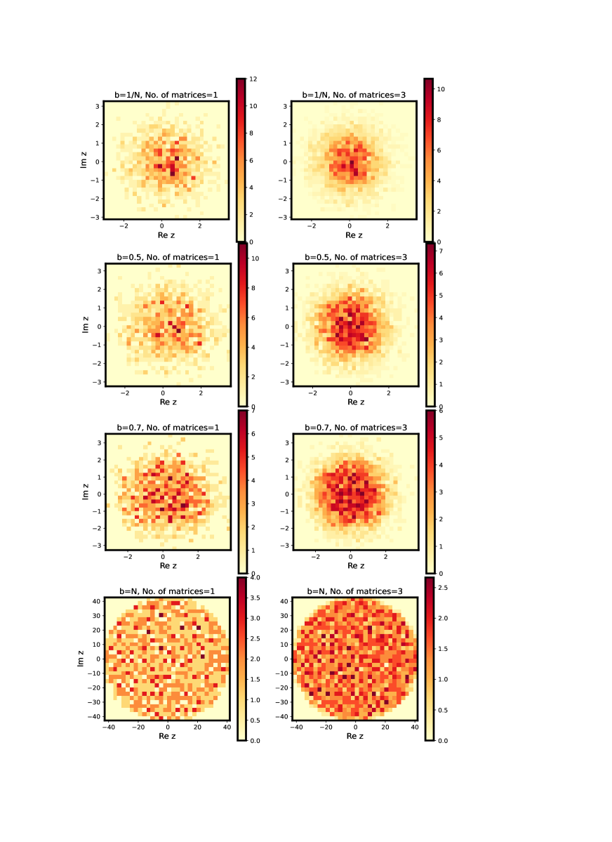
(ii) Ensembles with off-diagonal to diagonal variance decaying as a power law, referred here as just power law ensemble (PE) for brevity: . Eq.(9) now gives
| (83) |
with . Taking initial PE with then gives .
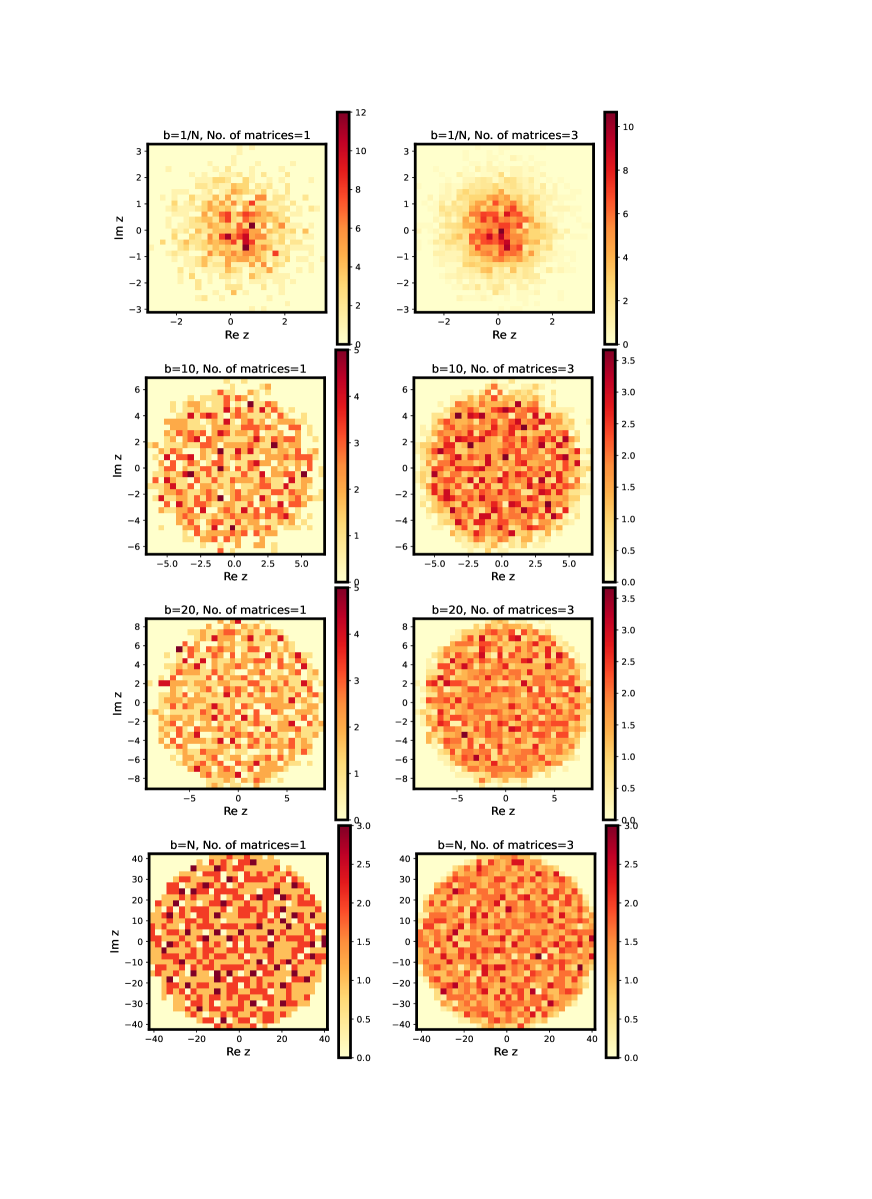
(iii) Ensembles with off-diagonal to diagonal variance decaying as an exponential, referred here as exponential ensemble EE: . Eq.(9) now gives
| (84) |
with same as in eq.(83). Taking initial EE with then gives .
As indicated above, while each ensemble depends on at least two system parameters, namely, and system size , the nature of that dependence varies significantly, from constant behavior to power law decay to exponential decay of the off-diagonals. More clearly the off-diagonals in the PE and EE case are also functions of the distance between basis-states, and thereby dependent on basis parameters. To understand the system dependence of the spectral density, we exactly diagonalize each ensemble for many values and for matrix size . The ensemble size i.e the number of matrices in each ensemble is chosen so as to give a smooth behavior and therefore depends on the specific measure. While the limit in each case corresponds to the Ginibre ensemble limit, the limit the Poisson statistics; a variation of therefore leads to a Poisson Ginibre crossover for each ensemble. Based on our theoretical prediction, the Ginibre limit is reached when almost all off-diagonals of a typical matrix in the ensemble become of the same order as the diagonals. As this occurs at different rates for BE, PE and EE, their -values for the Ginibre limit are different; (this is indeed due to role of hidden system parameters manifesting through different variance structure for each ensemble). With increasing , for each of the three cases mentioned above approach almost same value, with matrix elements distribution becoming identical. The eigenvalues are then expected to increasingly repel each other with increasing , thereby causing them to distribute uniformly on the complex plane. and approach the Ginibre limit. This is indeed confirmed by the figures 1-3, illustrating the variation of spectral density on the -plane as varies for BE, PE and EE respectively; here left panel depicts the behavior for a single matrix and right for . The rate of change with however is different for each case e.g. the approach to Ginibre limit is most rapid for EE case.
We recall that the Ginibre limit corresponds to the ergodic limit. It is therefore natural to seek whether the spectral density for each ensemble is indeed non-ergodic for smaller -values? To illustrate the latter, figures 1-3 display a comparison of the spectral and ensemble averaging for the spectral density in each ensemble for four -values. The spectral averaging here is obtained by considering the density of the eigenvalues of a single matrix on the -plane and the ensemble averaging by averaging over the spectral density of the eigenvalues for three matrices. As the illustrations in figures 1-3 indicate, even for a single matrix for large values (), appears almost same as as well as for all point on the complex plane reconfirming its ergodicity. As decreases, a deviation between the two cases is noticeable even visually; this indicates a non ergodic nature of the spectrum for small values in each case. However the approach of the spectral density to ergodic limit as increases is different for each ensemble.
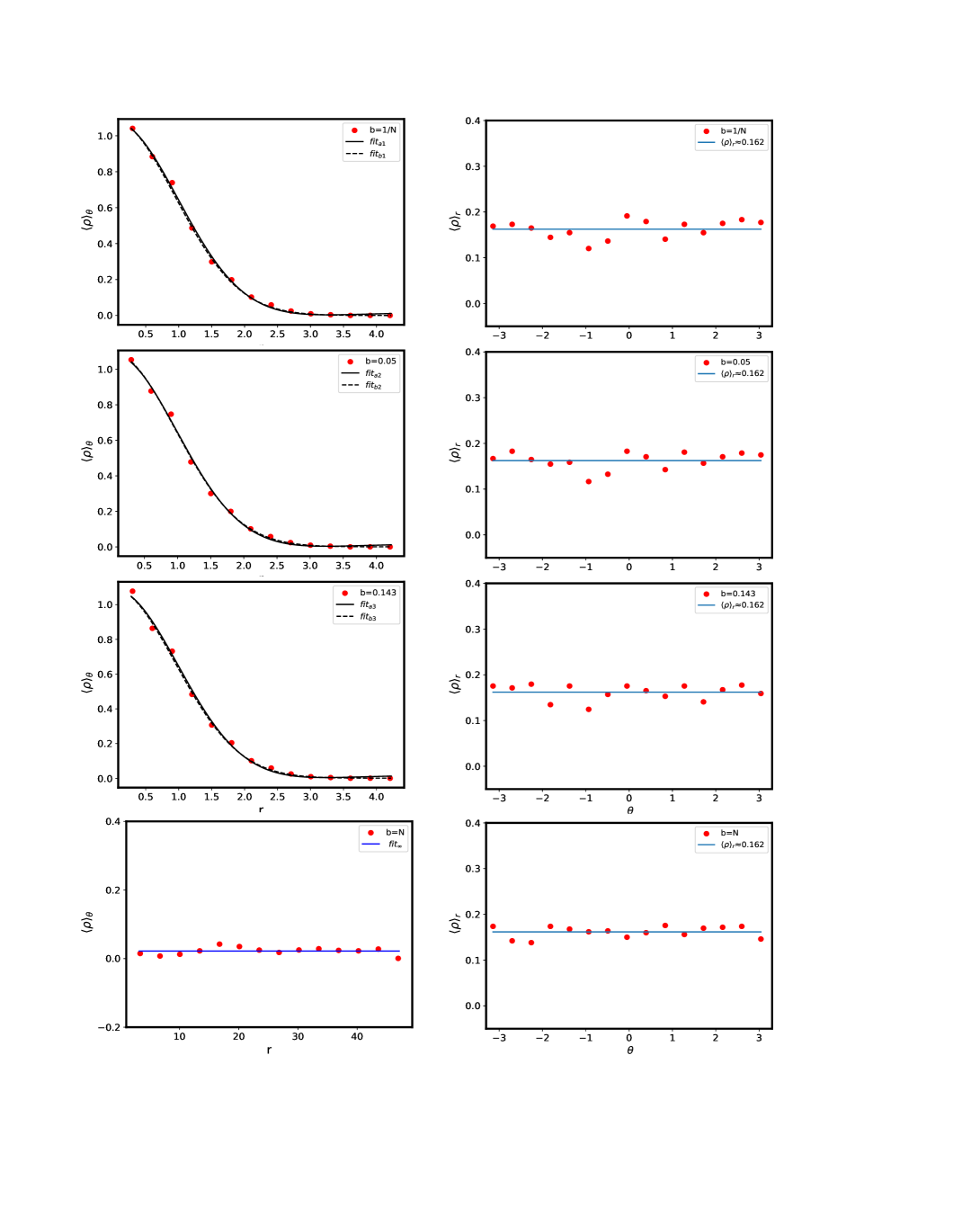
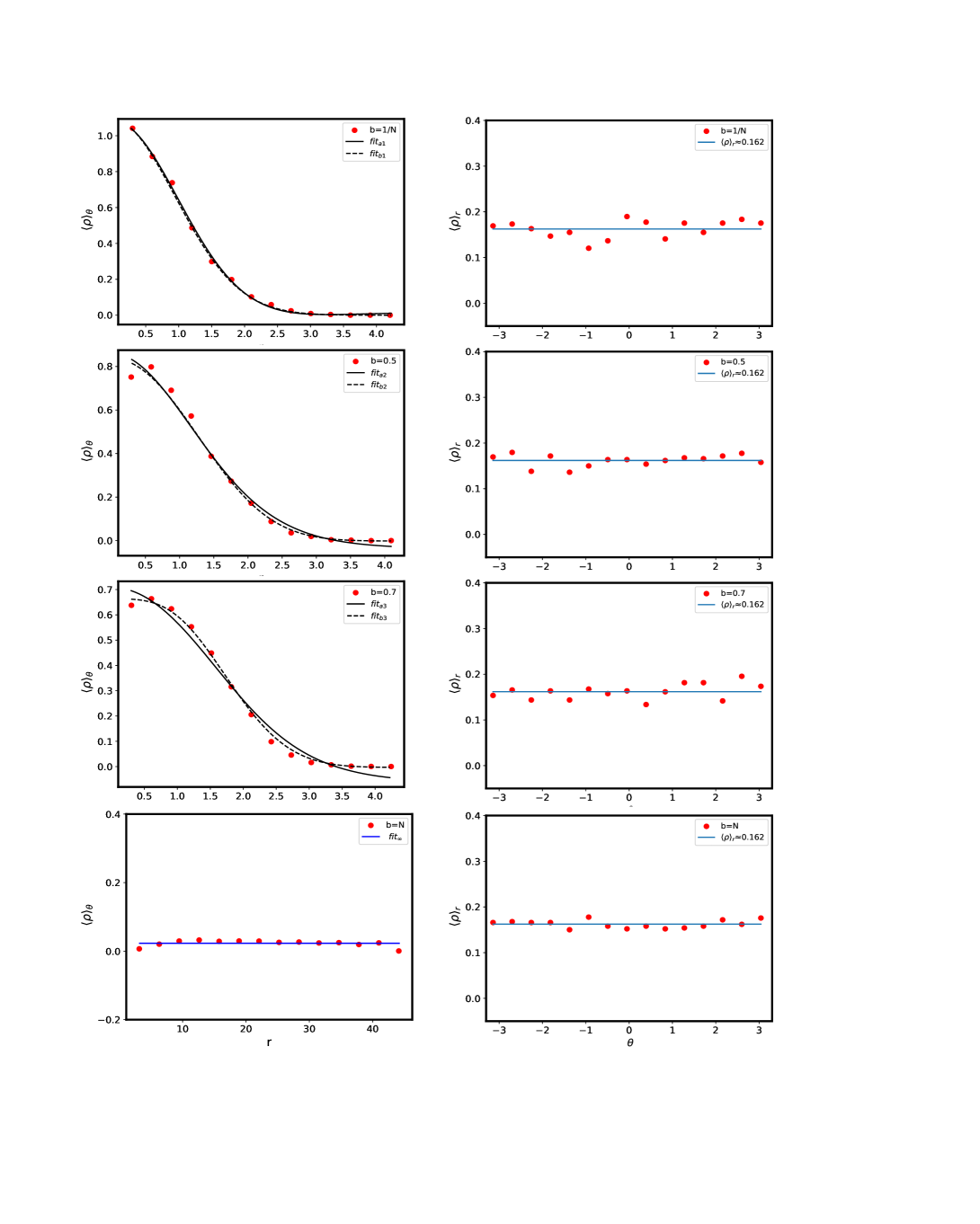
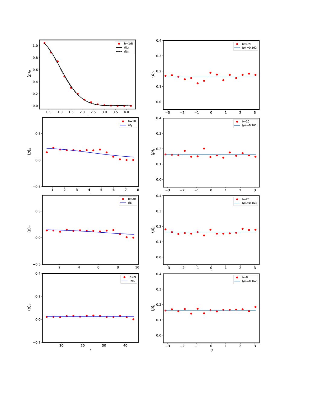
While the illustrations in figures 1-3 provide a qualitative insight about the behavior of spectral density on the complex plane., it is desirable to display the density in a way that could give better quantitative insights e.g. by analyzing its radial/ angular dependence separately. We also recall that the results obtained by our theoretical analysis are based on a separation of variables approach i.e by assuming along with as a particular solution of the evolution equation for . This in turn implies that and therefore a numerical averaging of over is expected to agree with our theoretical result for if the separability assumption is valid. Similarly and a numerical average of over is also expected to agree with our theoretical result for . As discussed in section IV. A, B, C as well as in appendix F, is almost constant in but varies with both and .
As mentioned above, the Poisson Ginibre crossover occurs at different rates for BE, PE and EE; it is therefore natural to seek the detailed role of in the crossover. For numerical analysis, we choose the initial condition for each ensemble mentioned above.; the choice is theoretically predicted to correspond to Poisson spectral statistics. (We note that the choice is arbitrary and one could equally well choose too). With Poisson ensemble as an initial condition, the approximation (used in section IV.C) is indeed valid for and also for small , thereby justifying use of eq.(60). The numerics for gives the initial density as
| (85) |
with as constants (the values for each ensemble given in table I). Using the above initial condition then suggest that (eq.(60)) decays exponentially or faster with . Thus using eq.(134) along with given by eq.(65) and , we have
| (87) | |||||
with . Here, to keep finite at , we need ; (this follows from the relation . valid for small ). As clear from the above, for small remains almost of the same form as the initial density except for a change of coefficients.
Further for large , the density is expected to reach uniformity on the complex plane within a circle of radius ; the appropriate in this case is therefore given by eq.(63). Using the latter in eq.(132), we have (now )
| (88) |
with .
Figures 4-6 display the -dependence of behavior for the three ensembles, each consisting of ten complex matrices of size and considered for four -values; (we note that the size of the ensemble is sufficient for the analysis of ). We numerically determine by counting the number of eigenvalues in an annular disk at a distance , of width and centred at and then rescaling the number by the area . The corresponding values in terms of for each case are obtained from eqs.(82, 83, 84) using , giving for BE, for PE, and, for EE. The specific values considered for each case and corresponding along with the fitted functions are given in table I. (Consistent with our theory, here we have for each case, increasing from as varies from ). We note, for the reference below, that for EE case becomes very large for all -values above , thereby implying a rapid transition from the initial state to Ginibre limit.
Figures 4-6 also display a comparison with eq.(87), eq.(87) for small -values and eq.(88) for . Although the includes infinite number of terms, we consider only first few terms (with ). Further, although the constants of can in principle be determined from the initial condition, the technical issues mentioned in appendix F leave us with no viable option but to determine them by numerical fitting; the values for the fitting parameters in each case are given in table I. As figure 4 for BE and figure 5 for PE indicate, varies slowly from its initial state and can be well fitted by eq.(87) for as well as for two intermediate values of with ; (as mentioned near eq.(65), theoretically can be arbitrarily small). The details of the parameters for fitted functions for each case are given in table 1 (labelled as ).
The figures 4 and 5 also indicate a good agreement with eq.(87) for intermediate -values (again keeping only first few terms of referred by ); this is expected due to slow change in for the chosen -values for BE and PE. Here required for comparison is obtained by fitting the case . We note however that a good agreement with eq.(87) for PE case, occurs for a different value than the one used for fitting with eq.(87); a possible explanation of this deviation could be attributed to numerical stability. (We also note that, for the initial choice as , it is not appropriate to use a theoretical prediction i.e a Poisson limit or the density of independent distributed eigenvalues on a complex plane for , and it should be determined numerically. This is because BE, PE and EE, defined above eqs.(82, 83, 84) respectively, are expected to approach exact Poisson statistics only in limit). As expected on theoretical grounds, the behavior for the remaining case i.e for BE and PE is almost constant and is fitted by eq.(88).
Contrary to BE and PE, the variation of with for EE case, displayed in figure 6, is quite rapid. Indeed it is well-fitted by eq.(88) for all three cases except for the case . This is expected because the dependence of for this case is almost negligible and becomes very large for all three values . This in turn also confirms the sensitivity of the spectral density to instead of .
Proceeding similarly, is numerically obtained, for a fixed , by counting the eigenvalues lying between sector and on the complex plane and then rescaling the number by the area of the sector. As predicted on theoretical grounds (discussed in section IV), is almost a constant for all considered values for each of the ensemble. We emphasize that an agreement of our theoretical predictions with fitted functional form for both and also lends credence to the separability ansatz made in section IV.
An important prediction of our analysis, mentioned in previous section and worth reemphasizing, is as follows: based on the complexity parameter formulation, can be described by the same mathematical form for a wide range of Gaussian ensembles e.g. with varying degree of the sparsity if they share the same -value and belong to same global constraints class although their local constraints may differ, resulting in different ensemble parameter values. The analogy however is not limited to a single static point on the evolutionary path; if a random perturbation subjects the ensemble to evolve, it continues lying along the same evolutionary path in the ensemble space (constrained by fixed values of based on global constraints). As each case displayed in figures 4-6 is well-described by either eqs.(87, 88) obtained from complexity parameter formulation of the spectral density, the above prediction is indeed well supported by our numerical results.
VI Conclusion
In the end, we summarize our main ideas and results discussed above along with some open questions.
Based on the representation by a multiparametric Gaussian ensemble of complex matrices, we find that the ensemble averaged spectral density of a non-Hermitian complex system is sensitive to system-specific details only through the complexity parameter, a single functional of the system conditions. A variation of system conditions may subject the spectral density to evolve in spectral as well as ensemble space, with global constraints e.g. conservation laws and symmetries act as the constants of dynamics. Our search for a path in the ensemble space, the evolution along which mimics that on the spectral plane, leads to a single parametric ”universal” path fixed by a set of global constraints. The relevance of such a path can be explained as follows: when system parameters vary, the ensembles, representing different systems subjected to same set of fixed global constraints, are confined to evolve along this path. This also describes a universal dynamics, in terms of the complexity parameter , for the eigenvalues of complex matrices (with Gaussian randomness) in an arbitrary initial state and subjected to mutiparametric perturbations equilibrium; the dynamics approaches the steady state of Ginibre ensemble for large -limits. More explicitly, as different complex matrix ensembles occurring at same point of this path (i.e those with same value of and similar initial statistics) have same statistical spectral properties, this indicates the hidden universality even in non-equilibrium regime i.e beyond Ginibre ensemble.
An important result of our analysis is the solution of the evolution equation for the average spectral density for arbitrary values of the complexity parameter. Although technical complexity of the differential equation made it necessary to assume the weak second order spectral correlations on the complex plane, the conjecture is based on the very definition of the local spectral correlations, expected to be weaker beyond a single local mean level spacing and is therefore valid for calculation of the average spectral density. Further, due to arbitrary choice of the ensemble parameters in our analysis, the solution is applicable to a wide range of ensembles e.g. various type of sparse matrix structures that describes the statistical behavior of non-Hermitian operators of complex systems e.g. many body or disordered systems. The above claim is indeed confirmed by the numerical analysis of three ensembles with different degree of the sparsity of the off-diagonals; we find that their numerically obtained average spectral densities agree well with our theoretical formulation in terms of the complexity parameter and based on separability conjecture.
We note that our present numerical analysis is based on the choice of initial condition corresponding to Poisson spectral statistics on a complex plane and is chosen due to intense current interest in the Poisson to Ginibre transition in spectral statistics, with intermediate state described by various sparse random matrix ensembles representing many real non-Hermitian systems. But as our evolution equations for the jpdf of eigenvalues, and thereby spectral density, are valid for any arbitrary initial condition, it is desirable to pursue a numerical verification for other initial conditions too. For example, the choice of an Ginibre ensemble of real asymmetric matrices as an initial condition would lead to a crossover/ transition between two different universality classes of Ginibre ensembles on complex spectral plane. Similarly the choice of any other universality classes mentioned in hkku as an initial condition would give rise to a different transition from the chosen initial statistics to that of Ginibre ensemble of complex matrices. Such studies are indeed expected to give new insights in the ergodic/ non-ergodic aspects of the spectral statistics.
Our study also gives rise to many other queries e.g. can the complexity parameter formulation and the universality in non-equilibrium regime be extended to non-Gaussian ensembles as well as to structured ensembles with correlated matrix elements? The information is relevant in order to model more generalized class of non-Hermitian systems where existence of additional matrix constraints can lead to many types of matrix elements correlations. Another very important question for application to many body non-Hermitian systems is how the behavior of correlations in the edge differ from the bulk? The information is needed to understand e.g. the non-Hermitian skin effect and the absence of conventional bulk-boundary correspondence in topological and localization transitions in non-Hermitian systems am and also for applications to biological neural networks. Another natural future extension of our analysis is to seek the explicit solution for the complexity parameter based evolution equation for the higher order spectral correlations on the complex plane. A similar formulation for the eigenvector correlations if possible is also desirable. We intend to answer some of the above queries in near future.
Acknowledgements.
One of the authors (P.S.) is grateful to SERB, DST, India for the financial support provided for the research under Matrics grant scheme.References
- (1) M. V. Berry, Czechoslovak J.Phys. 54, 1039, (2004).
- (2) D. S. Borgnia, A. J. Kruchkov, and R.-J. Slager, , Phys. Rev.Lett.124, 056802 (2020).
- (3) N. Okuma, K. Kawabata, K. Shiozaki, and M. Sato, Phys.Rev. Lett.124, 086801 (2020).
- (4) S. Yao and Z. Wang, Phys. Rev. Lett.121,086803 (2018).
- (5) M. S. Rudner and L. S. Levitov, Phys. Rev. Lett.102,065703 (2009).
- (6) Y. C. Hu and T. L. Hughes, Phys. Rev. B84, 153101 (2011).
- (7) K. Esaki, M. Sato, K. Hasebe, and M. Kohmoto, Phys. Rev. B84, 205128 (2011).
- (8) Z. Gong, Y. Ashida, K. Kawabata, K. Takasan, S. Hi-gashikawa, and M. Ueda, Phys. Rev. X8, 031079 (2018).
- (9) H. Schomerus, Opt. Lett.38, 1912 (2013).
- (10) Y. Ashida, Z. Gong, and M. Ueda, Advances in Physics 69, 249 (2020).
- (11) N.Moiseyev, Non-Hermitian Quantum Mechanics (Cambridge University Press, 2011).
- (12) B. Skinner, J. Ruhman, and A. Nahum, Phys. Rev. X9, 031009 (2019).
- (13) A. Zabalo, M. J. Gullans, J. H. Wilson, R. Vasseur,A. W. W. Ludwig, S. Gopalakrishnan, D. A. Huse, and J. H. Pixley, Phys. Rev.Lett. 128, 050602 (2022).
- (14) A. C. Potter and R. Vasseur, arXiv e-prints, arXiv:2111.08018 (2021), arXiv:2111.08018
- (15) J. Feinberg and A. Zee, Phys. Rev. E59, 6433 (1999).
- (16) L. G. Molinari, Journal of Physics A: Mathematical and Theoretical 42, 265204 (2009).
- (17) Y. Huang and B. I. Shklovskii, Phys. Rev. B 101, 014204 (2020).
- (18) K. Kawabata and S. Ryu, Phys. Rev. Lett.126, 166801(2021).
- (19) G. L. Celardo, M. Angeli, and R. Kaiser, arXiv preprint arXiv:1702.04506 (2017).
- (20) F. Cottier, A. Cipris, R. Bachelard, and R. Kaiser, Phys. Rev. Lett.123, 083401 (2019).
- (21) C. E. Maximo, N. A. Moreira, R. Kaiser, and R. Bachelard, Phys. Rev. A100, 063845 (2019).
- (22) A. Guo, G. J. Salamo, D. Duchesne, R. Morandotti, M. Volatier-Ravat, V. Aimez, G. A. Siviloglou, and D. N.Christodoulides, Phys. Rev. Lett.103,093902 (2009).
- (23) H.J.Sommers, A. Crisanti, H. Sompolinsky and Y. Stein, Phys. Rev. Lett., 60, 1895 (1988).
- (24) D.R.Nelson and N.M.Shnerb, 58, 1383, (1998).
- (25) K. Ranjan and L. F. Abbott, Phys. Rev. Lett., 97, 188104, (2006).
- (26) A. Amir, N. Hatano and D. R. Nelson, Phys. Rev. E 93, 042310, (2016).
- (27) Y. Ahmadian, F. Mumarola and K. D. Miller, Phys. Rev. E 91, 012820, (2015).
- (28) N. Hatano and D.R.Nelson, Phys. Rev. Lett. 77, 570 (1996); K.B. Efetov, Phys Rev. B 56 9630 (1997); I.Y. Glodsheild and B.A. Khoruzhenko, Phys. Rev. Lett., 80, 2897 (1998); C.Mudry, B.D.Simons and A.Altland, Phys. Rev. Lett., 80, 4257 (1998).
- (29) J.T.Chalker and Z.J.Wang, Phys. Rev. Lett. 79, 1797, (1997).
- (30) J.T.Chalker and B.Mehlig, Phys. Rev. Lett. 81, 3367, (1998).
- (31) P. Shukla, Phys. Rev. Lett. 87, 19, 194102, (2001).
- (32) C.M. Bender, N. Hassanpour, D.W.Hook, S.P.Klevansky, C. Sunderhauf and Z. Wen, Phys. Rev. A 95, (2017).
- (33) C.M. Bender and S. Boettcher, Phys. Rev. Lett. 80, 5243, (1998).
- (34) C.M. Bender, D.C. Brody and H.F.Jones, Phys. Rev. Lett. 89, (2002).
- (35) A. Mostafazadeh, J. Math. Phys. 43, 205, (2002); 43, 2814, (2002); 43, 3944, (2002).
- (36) Y.N.Joglekar and W.A. karr, Phys. Rev. E, 83, (2011)
- (37) E-M Graefe, S. Mudute-Ndumbe and M. Taylor, J. Phys. A: Math. Theo. 48, 38FT02, (2015).
- (38) I. Rotter, J. Phys. A: Math. Theo., 42, 153001, (2009).
- (39) I. Rotter, arXiv:1011.0645, (2010).
- (40) J. Ginibre, J. Math. Phys. 6 440, (1965).
- (41) F.Haake et al., Z.Phys. B, 88, 359, (1992).
- (42) Nils Lehmann and H-j Sommers, Phys. Rev. Lett. 67, 941, (1991).
- (43) Y.V.Fyodorov and H.-J. Sommers, J. Math. Physics (N.Y.), 38, 1918, (1997).
- (44) Y.V.Fyodorov, B.A.Khoruzhenko and H.-J. Sommers, Phys. Rev. Lett., 79, 557, (1997).
- (45) Y.V.Fyodorov and B.A.Khoruzhenko, Ann. Inst. Henri Poincare (Physique Theorique), 68, 449, (1998).
- (46) J. Feinberg and A.Zee, Phys. Rev. E 59, 6433, (1999)
- (47) L. Sa, P. Ribciro and T. Prosen, Phys. Rev. X, 10, 021019, (2020).
- (48) R. Hamazaki, K. Kawabata, N. Kura and M. Ueda, Phys. Rev. Res., 2, 023286, (2020).
- (49) G.De Tomasi and I. Khaymovich, Phys. Rev. B, 106, 094204 (2022)
- (50) O. Bohigas and M. P. Pato, J. Phys. A: Math. Theor. 46, 115001, (2013).
- (51) A. M. Garcia-Garicia, S. M. Nishigaki and J.J.M. Verbaarschot, Phys. Rev. E 66, 016132, (2002).
- (52) K. Suthar, Y-C Wang, Y-P Huang, H.H.Jens and J-H You, Phys. Rev. B 106, 064208 (2022).
- (53) A. M. Mambuca, C. Cammarota and I. Neri, Phys. Rev. E 105, 014305 (2022).
- (54) I. Neri and F. Lucas Metz, Phys. Rev. Research, 2, 033313 (2020).
- (55) F. Haake, Quantum Signatures of Chaos (Springer-Verlag, Berlin, 1991).
- (56) M. L. Mehta, Random Matrices (Academic, New York, 1991).
- (57) J.B. French, V.K.B. Kota, A. Pandey and S. Tomsovic, Annals of Physics, 181, 198 (1988).
- (58) T. Guhr, G A Muller-Groeling and H A Weidenmuller 1998 Phys. Rep. V 299 189
- (59) P. Shukla, Int. Jou. of Mod.Phys B (WSPC), 26, 12300008, (2012).
- (60) A. Pandey, Chaos, Soliton and Fractals, 5, 1275, (1995).
- (61) A. Pandey, Phase Transitions (Taylor and Francis), 77, 835 (2004).
- (62) T A Brody, J Flores, J B French, P A Mello, A Pandey and S S M Wong, Rev. Mod. Phys. 53 385 (1981).
- (63) P.Shukla, Phys. Rev. E 71, 026266 (2005).
- (64) P.Shukla, Phys. Rev. E 62, 2098, (2000);
- (65) P. Shukla, J. Phys.: Condens. Matter 17, 1653 (2005); J. Phys. A 41, 304023 (2008); Phys. Rev. E 75, 051113, (2007); J. Phys. A: Math. Theor 50, 435003 (2017).
- (66) R. Dutta and P. Shukla, Phys. Rev. E, 76, 051124 (2007); 78, 031115 (2008); M. V. Berry and P.Shukla, J. Phys. A 42, 485102 (2009). S. Sadhukhan and P. Shukla, Phys. Rev. E 96, 012109 (2017); P. Shukla, New J. Phys. 18, 021004 (2016). .
- (67) T. Mondal and P.Shukla, Phys Rev. E 102, 032131 (2020)
- (68) P.Shukla, J. Phys. A 41, 304023 (2008).
- (69) P. Shukla, Phys. Rev. B, 98, 054206 (2018).
- (70) F.L.Metz, I. Neri and T. Rogers, J. Phys. A: Math. Theor. 52, 434003, (2019).
- (71) I. I. Arkhipov and F. Minganti, Phys. Rev. A, 107, 012202 (2023)
- (72) M. G. Ansari and P. Shukla, arXiv:2312.08203 [cond-mat.dis-nn].
- (73) A.Pandey and P.Shukla, J. Phys. A, (1991).
- (74) N.M. Temme and E.J.M. Veling, Indagationes Mathematicae (Elsevier) 33, 1221, (2022).
- (75) Although at present we are not aware of any real physical non-Hermitian operator with phase singularity at on spectral plane , but such a situation can be envisaged to arise, for example, for a system with vanishing spectral density at .
Appendix A Complexity parameter formulation of
As discussed in section II. A, we seek a transformation from the set of parameters (with ) to another set , such that multiparametric evolution governed by the operator , defined in eq.(2), can be reduced to a single parameter evolution, say while rest of them i.e remain constant.
We redefine, for technical ease, the ensemble density as , with as the normalization constant of (such that ). Here is an unknown function of the parameters and such that satisfies the condition
| (89) |
The above in turn gives the condition to determine :
| (90) |
To fulfill the second part of the condition in eq.(89) i.e , must satisfy following condition
| (91) |
and
| (92) |
with defined in eq.(3).
The above set of equations can be solved by standard method of characteristics; the latter leads to a set of relations
| (93) |
and
| (94) |
Substitution of and from eq.(3) and rearranging eq.(93), we have, with ,
| (95) |
where . Solving the above set of equality relations in eq.(95), we have
| (96) | |||||
| (97) |
Substitution of in eq.(93), we now have
| (98) |
with where . The above on solving now gives
| (99) |
where with and given by the initial conditions. Under condition that all ensemble parameters are undergoing variation during evolution,one can set all equal e.g or thereby giving .
Appendix B Derivation of eq.(10)
Let be the probability of finding eigenvalues of between and for given sets and ,
| (101) |
with and or equivalently .. with .
For technical ease, we define . Using , this leads to
| (102) |
Differentiating eq.(102) both sides with respect to leads to
| (103) |
A substitution of eq.(5) in the above integral now gives
| (104) |
where
| (105) | |||||
| (106) |
Using repeated partial integration and the boundary condition that vanishes as and can be rewritten as
| (107) |
and
To proceed further, we need the information about the response of the eigenvalues as well as the eigenvectors to a small change in the matrix element . Using the eigenvalue equation with and as unitary matrices, the required relations can be given as follows
| (109) |
Appendix C Derivation of eq.(16)
An integration of eq.(10) over the variables (as well as their conjugates), multiplying both sides by and subsequently using eq.(15) leads to
| (110) | |||||
where
| (111) | |||||
| (112) |
with . The second relation in the above equation follows by noting that, for , can be taken out of the integral; subsequent use of eq.(15) then gives eq.(111). For , the repeated partial integration over along with the boundary condition that as gives eq.(112).
Appendix D Derivation of eq.(17)
Using standard transformation rules from cartesian to polar coordinates i.e , , we have , , we then have
| (120) | |||||
| (121) |
where and . Writing in term of and using and in eqs.(118, 119), and can now be rewritten as given in eq.(20) and eq.(21). Substitution of eq.(120) and eq.(121) in eq.(115) then gives eq.(17).
Appendix E Determination of from a given initial spectral density
As our solution of the dynamical equation for discussed in section IV is -range specific and therefore gives different conditions to determine unknown coefficients for small, large and finite regimes but with decaying angular correlations. As discussed below, here we consider two cases of initial conditions as examples.
(i) Gaussian decay of initial density with circular symmetry:
As an example, we consider the initial ensemble with
| (122) |
Small : Substitution of the above in eq.(35) and using leads to the condition, valid only for ,
| (123) |
Using the definition for , satisfies the relation and can now be obtained by an inverse Mellin transform.
Large : To determine unknown coefficients in our large -solution given by eq.(51), we now have the condition
| (124) |
with given by eq.(47) with and defined in eq.(49). Clearly the condition can be fulfilled only if and therefore we must have for . This in turn reduces the above as
| (125) | |||||
A comparison of the two sides of the above equation now gives and for and .
Finite : Using eq.(66) for along with eq.(127) ), eq.(66) gives for case C.(i),
| (126) |
with given by eq.(63), eq.(64) and eq.(65) based on . With its right side -dependent and the left side independent, the condition eq.(126) can be fulfilled only for . The latter leads to the condition .
The standard route to determine constants from equations such as above is based on using orthogonality of functions appearing in the series. However as the same are not known in case of confluent Hypergeometric functions, one option left to us is to expand both sides in power series and compare the terms on both sides.
(ii) Case for initial density used in numerical analysis:
The initial condition used for our numerical analysis correponds to for each of the three ensembles. As displayed in figures 4-6 for cases for BE, PE and EE, the spectral density in this case is as follows:
| (127) |
As in the previous case, here again we consider three different regimes to determine the coefficients.
Small : Using eq.(35), for along with eq.(127) (with ), we have,
| (128) |
Solving the above now gives .
Large : Using eq.(51), for along with eq.(127) (with ), we have for large ,
| (129) |
with given by eq.(47). As the left side of eq.(129) does not depend on , this implies for . The condition in eq.(129) now reduces as
| (130) |
Finite : Using eq.(66) for along with eq.(127) and ), eq.(66) now gives for case C.(i),
| (131) |
with given by eq.(63), eq.(64) and eq.(65) based on . Here again -independence the left side of eq.(131) requires for . The condition in eq.(131) now reduces to . The constants in can again be determined, in principle, by inverting the condition with help of orthogonality relations of the mathematical functions appearing in or by expanding both sides as a power series and comparing the terms with same powers.
Appendix F Calculation of and
Using the functions and , the radial and angular dependence of can separately be analyzed.
Radial Dependence: Using the definition eq.(66) we have
| (132) |
with for the case and and for the case decaying exponentially or faster.
For small , we can approxmate . This implies, for small ,
| (133) | |||||
| (134) |
where .
For , the terms with increasingly lower values of begin to dominate the above sum, with only term contributing in . For large , the above series can then be approximated by retaining only some lower values of i.e
| (135) |
Determination of coefficients: Eq.(132) gives ; the unknown constants and of can then be determined from the initial condition. For example, for initial density given by eq.(127), we have (using eq.(65))
| (136) |
Using and expanding both sides in a power series near and comparing various powers of , we have and
| (137) |
where . Here is a Pochhammer symbol i.e .
Eq.(137) can further be written in form of a matrix equation with and as the column vectors, , (both ) and as an infinite dimensional matrix with entries . Inverting the above gives and thereby for each . In practice however inversion is not easy due to infinite dimansionality of the matrices involved, leaving the determination of the constants only by numerical fitting.
Angular Dependence: From eq.(66), we also have
| (138) |
where is independent of : with and dependent on (eq.(60)). As clear from the above, the dominant contribution to eq.(138) comes from term, thereby suggesting ; this is consistent with our numerical results, displayed in figures 4-6, indicating almost constant in .
.
, for ,
, for ,
, for
| b | Fits for BE case (figure 4) | |
| 1/N | 0.00 | |
| 1/20 | 7.88 | |
| 1/7 | 9.98 | |
| N | 26.34 | |
| b | Fits for PE case (figure 5) | |
| 1/N | 0.00 | |
| 0.5 | 12.46 | |
| 0.7 | 13.12 | |
| N | 24.46 | |
| b | Fits for EE case (figure 6) | |
| 1/N | 0.00 | |
| 10 | 9.16E10 | |
| 20 | 9.16E10 | |
| N | 9.16E10 |