Automatic Tree Ring Detection using Jacobi Sets

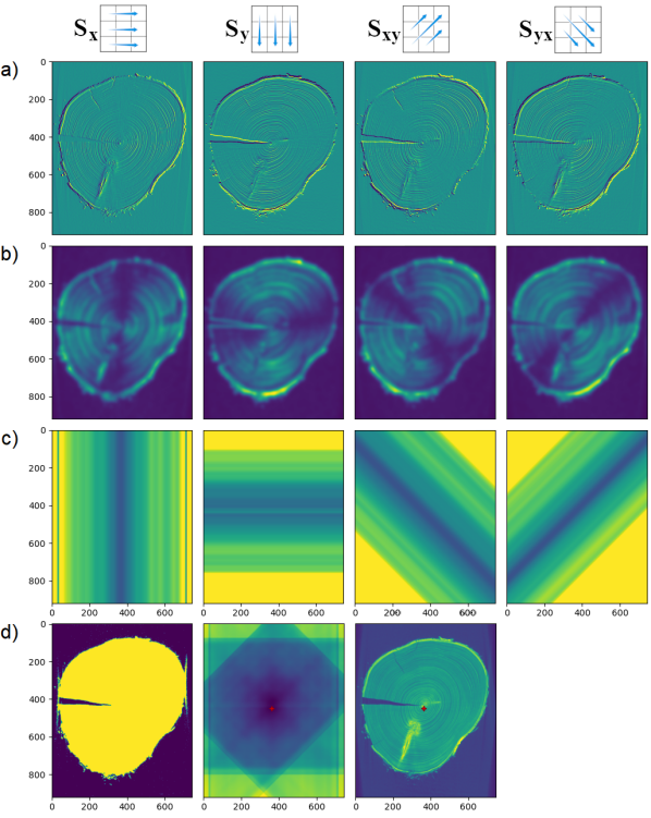
The first task is to find the center, or pith, of the given tree disk; an example of this procedure is shown in Fig. 2. Our proposed method of center location relies on Sobel filters, which is a derivative mask commonly used for feature detection in computer vision [9]. The goal of the Sobel filter is to approximate gradients in an image, so pixels with the highest magnitude of gradient can be designated as belonging to edges. The Sobel operator is defined in the horizontal and vertical direction, as well as the two diagonal directions by $3\times 3$ convolution kernels $S_{x}$, $S_{y}$, $S_{xy}$, and $S_{yx}$:

For a single two-dimensional slice, consider the Sobel filter based on $S_{x}$, shown in the top left of Fig. 2. This filter assigns higher absolute values to vertical edges. In the context of tree rings, we expect very few vertical edges at the $x$-coordinate of the center (since tree rings cross that $x$-coordinate in a perpendicular fashion), and more or longer vertical edges at $x$-coordinates further away from the tree center. In particular, we expect the Sobel filter in a given direction to produce, on average, higher absolute values at coordinates (in that direction) away from the center; see row (b) of Fig. 2. In order to ignore edges that occur in the background of the image, we identify the pixels that are part of the tree disk using a mask. Such a mask can viably be obtained using a threshold intensity when using X-ray CT scans, as well as when working with pictures taken against a contrasting background. The used mask is shown in the left column of row (d) of Fig. 2.

After blurring the absolute values resulting from the Sobel filter, we take, at a given $x$-coordinate, the average over all pixels that lie on the tree disk, see row (c) of Fig. 2. If for a given $x$-coordinate, fewer than a threshold number of pixels (100 in our case) lie on the tree disk, we default to the maximum value over the image, rather than the average at that $x$-coordinate. This results in a function that assigns to any $x$-coordinate, a quantity representing how vertically oriented the rings at that $x$-coordinate are. We similarly compute a function that represents how horizontally oriented the rings are at a given $y$-coordinate, and similar functions for the two diagonal directions; shown in rows (a-c) of columns 2-4.

Intuitively, two such functions can be combined to locate the center of the disk: look for the $(x,y)$-coordinate with a minimum number of rings oriented vertically at the $x$-coordinate, and a minimum number of rings oriented horizontally at the $y$-coordinate. However, considering only the $x$- and $y$- directions is not very robust, as radial cracks may form in disks cut from felled trees, as can be seen in the Red Cedar disk, Fig. 1. This creates an edge that is oriented in the direction perpendicular to that of the rings at a given $x$- or $y$-coordinate, and may give the function an undesirably high value at the center of the disk. To remedy this, we also use the diagonal directions, as it is unlikely for a disk to have cracks in multiple directions. In our final step (see Fig. 2, row (d), columns 2 and 3), we sum for each pixel, the four directional functions at the corresponding coordinate, and identify the location of the pixel with minimum value as the center of the disk.

In the case of a 3D image, we can repeat this process for every 2D slice, and take a line of best fit to ensure that the centers move continuously between adjacent slices. Given the center of a particular 2D slice, we transform the slice into polar coordinates, so that $y$-coordinates correspond to angles, and $x$-coordinates correspond to distance from the center. To avoid loss of information around the edges of the images, we pad the top of the image with rows from the bottom of the image. These padded polar images represent the end of the preprocessing stage and are shown in Figure 3.

The next step in the tree ring analysis is to detect the ring boundaries, which is a problem of edge detection in image processing.

For our tree disk scans, we consider two functions associated with the polar image.

1. 1.

   The intensity value $f(x,y)$ of a 2D grayscale image can be interpreted as a continuous function (by interpolating between adjacent pixels) from a 2D domain.

2. 2.

   The $y$-coordinate $g(x,y):=y$ of pixels of a 2D image can similarly be interpreted as a continuous function with the same domain.

To detect ring boundaries, we use a method based on Jacobi sets [5]. The Jacobi set of two real-valued functions with the same domain (such as the ones defined above) is defined as the set of critical points of one function restricted to the level sets of the other. For our functions $f$ and $g$, the Jacobi set corresponds to (a) the local minima and maxima of intensity value at any fixed $y$-coordinate, as well as (b) the critical values of $g$ on components of a fixed intensity. For two sufficiently well-behaved functions (i.e. Morse functions), the Jacobi set forms a collection of paths [5], which we can think of as ridges and valleys of type (a), pairs of which end at points of type (b). These ridges and valleys are shown for Red cedar in Fig. 4. In most conifer trees, the ridges correspond to ring boundaries. However, in some species, such as the Spartan sample, the valleys indicate rings boundaries.

Area-based persistence [13] is applied to the Jacobi results as follows in order to clean up noise and assign high values to ridges based on their persistence. Area-based persistence works by assigning a persistence value to each pixel. For a particular pixel $p$, this assignment is based on the intensities of pixels in its row (i.e. the restriction of $f$ to the $y$-coordinate of that pixel). If the intensity of $p$ is not a local minimum (in its row), the persistence value of $p$ is zero. On the other hand, if $p=(x_{p},y_{p})$ is a local minimum, we locate the closest pixels $\ell=(x_{l},y_{p})$ and $r=(x_{r},y_{p})$ to its left and right that have less intensity (so that $f(x,y_{p})\geq f(x_{p},y_{p})$ for $x$ between $\ell$ and $r$), and compute the areas

under the intensity function above the intensity of $p$, see Fig. 5. The persistence value of pixel $p$ will be the area of the smaller side: $\min\{A_{\text{left}}(p),A_{\text{right}}(p)\}$. Intuitively, more significant local minima (valleys) will lie between mountains that are high (in terms of area), so significant minima will be assigned a high persistence value. A symmetric method can be used to find persistent ridges (maxima). The persistence value of a minimum (or maximum, depending on the type of tree) corresponds to the certainty with which we call it a tree ring boundary. As such, we mark all minima or maxima that have at least some threshold persistence value as ring boundaries.

In the next section, we explore different threshold values, and validate our method against manually called ring boundaries, as well as state-of-the-art software. Results of persistence with different choices of thresholds and blur parameters are shown in Fig. 6 for the red cedar disk, and in Fig. 7 for the Spartan disk.

We use a traditional form of the edit distance [17] to compare sequences of tree ring widths. For each run of the scoring code, two text lists of x-values are compared using matching and costs based on distance. Once pairs are matched, the algorithm places a cost on each of three operations: 200 to add a point (resolve false negative), 200 to remove a point (resolve false positive), and the distance in pixels between two points to move a point (resolve minor errors in placement). The choice of 200 is high enough to make missing or false rings the dominant factor in the cost, and low enough to still be affected by placement errors. Note that the positions of the rings in the ground truth data set are marked by the researcher and thus are also subject to human error.

We examine edit distance costs for various combinations of the three aforementioned parameters: pre-threshold, blur, and post-threshold. Both thresholds range from $0$ to $0.2\cdot n$ where $n$ is the maximum intensity value in the image. The blur value is the value of $\sigma$ in a Gaussian blur filter, which indicates the standard deviation for the Gaussian kernel. Exploring these options between species allows us to consider which parameters can be fixed and which will need to be input or determined by the image. Costs for various parameter combinations with fixed blur value are shown in Figure 8. A higher blur value for the Spartan sample performs better, likely due to the increased space between rings as compared to the Red Cedar sample. The results with the minimum cost for Red Cedar are shown in Figure 6, and for Spartan in Figure 7. The matching for these results is shown in Figure 9.

MtreeRing is a newer open-source program in R for tree ring analysis which compares favorably with prominent software such as WinDENDRO™ [15]. We compare our results with MtreeRing using the edit distance cost we have developed.

For the same row on the same slice of each tree sample, we compute the tree ring boundaries using both our method and MtreeRing. For the Red Cedar sample, the output of our program has a cost of 964 whereas the MtreeRing LinearDetect output costs 2841. For the Spartan sample, our cost is 2213 and MtreeRing has cost 2661.

References

- [1] Salvador Arenas-Castro, Juan Fernández-Haeger and Diego Jordano-Barbudo “A Method For Tree-Ring Analysis UsingDiva-GisFreeware On Scanned Core Images” In Tree-Ring Research 71.2 Tree-Ring Society, 2015, pp. 118–129 DOI: 10.3959/1536-1098-71.2.118
- [2] Franco Biondi “From Dendrochronology to Allometry” In Forests 11.2 MDPI AG, 2020, pp. 146 DOI: 10.3390/f11020146
- [3] Andrew Bunn “A dendrochronology program library in R (dplR)” In Dendrochronologia, 2008
- [4] Herbert Edelsbrunner and John Harer “Jacobi Sets of Multiple Morse Functions” In Foundations of Computational Mathematics, 2002
- [5] Herbert Edelsbrunner and John Harer “Jacobi sets of multiple Morse functions” In Foundations of Computational Mathematics, 2004, pp. 35–57
- [6] Anna Fabijańska and Małgorzata Danek “DeepDendro - A tree rings detector based on a deep convolutional neural network” In Computers and Electronics in Agriculture 150C, 2018 DOI: 10.1016/j.compag.2018.05.005
- [7] C. Ferguson “Concepts and Techniques of Dendrochronology”, 1970
- [8] Ernst-Detlef Schulze Fritz H. “Atlas of Woody Plant Stems” Springer-Verlag Berlin Heidelberg, 2008
- [9] N. Kanopoulos, N. Vasanthavada and R.. Baker “Design of an image edge detection filter using the Sobel operator” In IEEE Journal of Solid-State Circuits 23.2, 1988, pp. 358–367
- [10] W. Lara and Felipe Bravo “measuRing: An R package to measure tree-ring widths from scanned images” In Dendrochronologia, 2015
- [11] “Lignovision™” RINNTECH® RINNTECH®
- [12] Elizabeth Munch “A User’s Guide to Topological Data Analysis” In Journal of Learning Analytics 4.2, 2017 DOI: 10.18608/jla.2017.42.6
- [13] Tim Ophelders, Willem Sonke, Bettina Speckmann and Kevin Verbeek “Kinetic volume-based persistence for 1D terrains” In 35th European Workshop on Computational Geometry (EuroCG), 2019, pp. 38:1–38:7
- [14] C.. Rueden, J. Schindelin and M.C. al. “ImageJ2: ImageJ for the next generation of scientific image data” In BMC Bioinformatics 18.529, 2017 DOI: 10.1186/s12859-017-1934-z
- [15] Jingning Shi, Wei Xiang, Qijing Liu and Sher Shah “MtreeRing: An R package with graphical user interface for automatic measurement of tree ring widths using image processing techniques” In Dendrochronologia, 2019
- [16] James H. Speer “Fundamentals of Tree-ring Research” University of Arizona Press, 2010
- [17] Carola Wenk “Applying an edit distance to the matching of tree ring sequences in dendrochronology” In Annual Symposium on Combinatorial Pattern Matching, 1999 DOI: 10.1007/3-540-48452-3˙17
- [18] “WinDENDRO™2019a” Regent Instruments Inc. Regent Instruments Inc.