Automatic Construction of Lane-level HD Maps for Urban Scenes

Yiyang Zhou^∗¹ and Yuichi Takeda^∗² and Masayoshi Tomizuka¹ and Wei Zhan¹ ^∗Both authors contributed equally to this work.¹Mechanical Systems Control Lab, University of California, Berkeley, CA, USA, 94705²Nissan Motor Co. Ltd., 1-1 Morinosatoaoyama, Atsugi, Kanagawa, 243-0123, JapanCorrespondence: [email protected]

Abstract

High definition (HD) maps have demonstrated their essential roles in enabling full autonomy, especially in complex urban scenarios. As a crucial layer of HD maps, lane-level information is especially useful to facilitate perception, localization, prediction and planning. However, the large scale deployment of HD maps is restricted by tedious human labelling and high maintenance costs, especially for urban scenarios with complicated road structures and incomplete lane markings. This paper proposes an approach based on semantic-particle filter to tackle the automatic lane-level mapping problem in urban scenarios. The method performs semantic segmentation on 2D front-view images and explores the lane semantics on a birds-eye-view image with true topographical projection. Exploiting OpenStreetMap, we further infer lane topology and reference trajectory at intersections with our mapping output. The proposed algorithm has been tested in densely urbanized areas, and the results demonstrate accurate and robust reconstruction of lane-level HD maps.

I INTRODUCTION

High definition (HD) maps have become a crucial component for full autonomy in a variety of complex scenarios. Encoded with accurate and comprehensive information of the static environment, HD maps can significantly facilitate perception, localization, prediction and planing [SEIF2016159]. HD maps contain multiple layers of information abstractions, and the lane-level information is of significant importance for many applications. Embedded with lane geometries, road semantics, and connection topology, the lane layer can be utilized for defining potential region of interest (ROI) for object detection [ZieglerJulius2014MBDA, Yang2018HDNETEH], regulating the lateral location of the ego vehicle [ubermaploco, HDlocoParticle, takedaloco], and predicting behavior of other vehicles [gao2020vectornet].

With numerous alluring applications, these lane-level HD maps, however, do not scale easily. Many of these HD maps are restricted to small scale environments due to the high costs in manual labelling and maintenance [paz2020probabilistic]. Recently, a few commercial products have been launched to automatically map highways [nvidiaDriveMap], where the lanes are structured and the markings are clear. In urban scenes, however, the road may have complicated forking, potholes, broken markings or even no markings at all. Also, the topological relationship of urban lanes are much more intricate. Figure 1 shows several urban lane markings exemplar in California. As a result, the automatic lane-level mapping problem in urban areas remains as an open and challenging problem.

In this paper, we propose a method based on semantic-particle filter to automatically generate an urban lane-level HD map with camera and LIDAR (optional). The proposed method contains three major components: a semantic segmentation network for scene understanding, a bird’s-eye-view (BEV) re-projection and sequential Monte Carlo lane tracing module, and a intersection lane inference module with OpenStreetMap (OSM) [OSM]. The whole pipeline employs public datasets to enable semantic understanding, and it only requires one single execution per road direction for a complete reconstruction of the lane-level details including the lane boundaries, reference trajectories, lane splitting information, and road topology. Lastly, we represent our generated lane map in a differentiable format for downstream modules. Exemplar mapping results can be seen in Figure 1. We test the proposed method in densely urbanized areas such as San Francisco and Downtown Berkeley, and the results demonstrate an accurate and robust construction of the lane-level HD maps.

Refer to caption — Figure 1: Urban roads are complicated: lane splitting (A), broken or no markings (B and C), and complicated intersections (D). Urban intersections are even worse: shown in C is a 6-way intersection in San Francisco. The proposed algorithm can explore the lane structure and intersection topology in such complex environments.

The major contributions of this paper are:

•

Proposed to combine semantic scene understanding with Monte-Carlo sequential exploration for accurate and robust map construction for urban roads.
•

Exploited OSM as a coarse prior map, from which we constructed refined intersection topology and geometry.
•

Tested the proposed algorithm in densely urbanized area and validated the robustness and accuracy.

II RELATED WORKS

With the HD Map-related research advancing in the past few years, there are a number of attempts for automatic lane mapping in different scenarios. Here we list related works for different modules of the mapping problem.

II-A Lane detection: markings

Since the lanes are defined by the lane markings painted on the road surface, a natural way for lane-level map construction initiated from the lane marking detection perspective. Nieto et al. used a step-row filter [steprow] for lane marking detection and applies Rao-Blackwellized Particle Filter for lane tracing [NietoReal-timeFilter]. In [Li2017DeepScene], Li et al. used Convolutional Neural Network and Recurrent Neural Network for lane marking detection on highways. More recently, Garnett et al. [Garnett20193D-LaneNet:Detection] and Guo et al. [GuoGen-LaneNet:Detection] further used the 3D-LaneNet framework not only to classify the lane in an image, but also predict its location in 3D.

These approaches achieve high quality marking detection in highway or suburban roads where the shape of the roads are simple and can be approximated by a polynomial-like functions. However, it is hard to implement the aforementioned methods to urban scenarios with complicated road structures, broken/missing lane markings, and frequent road splits. Furthermore, the method mentioned in [Garnett20193D-LaneNet:Detection] and [GuoGen-LaneNet:Detection] only works for scenarios with mild changes in 3D slope, disregarding the abrupt changes in road topography.

II-B Lane detection: drivable areas

Some other methods focus the drivable areas for lane detection. Meyer et al. designed a specific neural network for ego and neighboring lane detection [Meyer2018DeepDriving]. Kunze et al. created a scene graph from the the semantic segmentation result of the front camera to generate a detailed scene representation of the drivable areas and all road signage [Kunze2018ReadingScenes]. On the other hand, Roddick et al. used a pyramid projection network to extract the drivable area as well as other vehicles [RoddickPredictSemanticMap]. Neither of these methods were extended to the HD mapping domain, allowing a third vehicle to make full use of the detection results.

II-C Intersection lane inference

Understanding the intersection structure is an indispensable technique for autonomous driving and HD Map generation. Thus a number of studies have been conducted to extract invisible lanes and connecting topology at intersections.

Trajectories of other vehicles have been commonly used for intersection exploration. For example, in [Geiger20143DPlatforms] [Joshi2014JointStructure], the authors used vehicle trajectory acquired from on-board sensor such as LiDAR or stereo camera. Later, Meyer et al. reduced the dependency on accurate trajectory of other traffic participants and used a Markov chain Monte Carlo sampling to reconstruct the lane topology and geometry in an intersection [Meyer2019AnytimeParticipants]. In [Roeth2016RoadMeasurements, Chen2010ProbabilisticTraces], the authors used collected GPS data loaded on fleet vehicles. These methods have the potential to estimate lane-level structure of intersection, but they are data-hungry, and the performance relies heavily on the quality of the GPS data.

II-D HD map generation

Large-scale map generation has been long considered as a Simultaneous Localization and Mapping (SLAM) problem [Yang2018AMapping]. However, instead of semantics, common SLAM algorithms focus more on the odometry. Recently, in [paz2020probabilistic] and [elhousni2020automatic], the authors used semantics in the image domain and fuse semantic results with LIDARs to generate an semantic representation of the scene, not exactly an HD map. In terms of lane level map generation, a common approach is to accumulate extracted road environments along localization results [Guo2016ASensors, Joshi2015GenerationLaneLevelMaps]. Both aforementioned approaches used LiDAR to extract road environments, and used OSM as a map prior. In [Joshi2015GenerationLaneLevelMaps], fork and merge of the lanes were able to be recognized by particle filter based lane marking tracking. Homayoundar et al. on the other hand, used a directed acyclic graph (DAG) and treated each detected lane marking as a node to decide future actions for connection, initiation, or termination [Homayounfar2019DAGMapper]. However, these methods focused on road segments ignoring intersections, and they do not define the start and end point of the lanes. Thus, connections between lanes are not studied in these works. With the help of aerial images, authors of [Mattyus_2016_CVPR] studied both road sections and intersections. However, the method is limited by the availability and resolution of aerial images.

While the aforementioned efforts in lane detection and map generation has significant contributions to the community, they are limited to either simple road structures or single road segments. Our work targets specifically at the complicated urban driving scenes and considers both lane segments and intersection inference. Furthermore, we consider the topographical deformation of the road surface for more robust and accurate lane detection.

III PRIMITIVE: MAP HIERARCHY

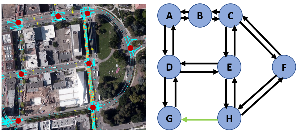
We depart from a topological point of view for this cartography task. A city road network is consisted of individual road segments and connecting intersections. As shown in Figure 2, this network could be further abstracted into a directional cyclic graph representation with each edge representing a directional road and each node representing a connecting intersection. We deliberately choose to have an edge for each direction because of the ubiquity of one-way roads and physically separated two-way roads in urban scenes. Previous works focused on either the edge or the node for geometrical information extraction, but we studied both parts geometrically and connect them in a graph network.

In the proposed method, we extract a coarse road-level topological information from OSM [OSM]. Disregarding the direction of travel for most roads, the OSM defines a road as a series of nodes connected together under a road instance. For special two-way roads with solid barrier as the median, OSM would have one road instance for each direction. Furthermore, the OSM defines an intersection as the connection node of two or more road instances. Although represented by a single node, the actual intersection is a geometrical region where multiple roads/lanes intersect. Utilizing such definition, we predict the intersection area with a polygon formed by the closest road node to the intersection node, leaving the rest of the road nodes as part of the atomic road. Figure 3 a-b demonstrate the separation of atomic roads and intersections.

With the atomic road and intersection patch defined as the skeleton of our map, we are able to match the moving data collection vehicle to an atomic road or an intersection in the road network. Now we proceed to the proposed methodology for automatic map generation.

IV METHOD

To automatically generate the lane-level map in densely urbanized areas, our proposed approach takes in signals from the on-board camera and LIDAR (optional) and utilizes OSM as the skeleton for our road network. As shown in Figure 4, the proposed method consists of three major components: semantic segmentation of the camera image, BEV accumulation and particle filter lane exploration, and intersection lane inference. In corresponding maps, we started with a coarse OSM map skeleton, went through the road semantic and reference trajectory generation, and ended with a lane-level HD map.

IV-A Semantic understanding of the scene

Drivable areas and lanes are defined by the road markings painted on the road surface. Although there are many previous works for detecting lane markings from cameras or LiDAR, they are mostly focusing on straight road such as highway, where the shape of lane markings are able to approximate by simple polynomial-like functions. However, lane markings in the urban area are more complicated: as shown in Figure 1, there are numerous lane splitting (A), and frequent stop lines (D). More importantly, a lot of roads in urban environment have broken or no road markings at all (B and C).

Therefore, instead of only extracting lane markings from camera images, we consider this problem as a semantic segmentation problem and infer both drivable area and lane markings from camera images. We are particularly interested in ego lanes, 2 neighboring lanes on each side of the ego lane, dashed lanes, solid lanes, stop lines, and cross-walks. These semantic instances forms the foundation to our understanding of the current drivable area. Considering both lanes and lane markings is especially efficient for urban scenes as the lane markings might be missing, and some drivable areas may be confused with parking zones. Outputs of this network are lane markings, and these drivable areas are shown in the semantic understanding module of Figure 4.

IV-B BEV accumulation and atomic road structure estimation

After the road semantics are extracted from camera images, these semantics are projected to the ground plane of map coordinates. These projected BEV views are then accumulated together for each semantic segments mentioned in Section IV-A to form a base for geometrical representation of the atomic road. For the scope of the semantic mapping problem, we assume that the pose of the ego vehicle is given from auxiliary sensors or algorithms.

For the BEV projection, most previous works assume a flat ground as the general road model. Thus, given the intrinsic and the estimated camera height, one could easily project the image onto the ground as shown in 5-b. However, such estimation is over-simplified in the city scenes as the road is not always flat. For urban areas, undulating road surfaces, either purposefully designed for draining purposes or accidentally caused by lack of maintenance, are common. Some poorly maintained roads even has potholes. 5-b shows that by simply assuming a flat surface of the road, the BEV projection could be largely distorted.

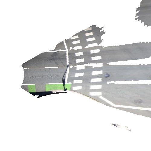
We propose to optionally use a corresponding LIDAR scan for ground topography estimation, and then project the image on to such topography mesh for better results. To generate the ground mesh from sparse point clouds, we process the synchronized LIDAR point cloud through a Delaunay Triangulation supported by [opencv_library]. The generated triangular mesh for the scene could be seen in 5-a. After topography correction, the BEV projection could be seen in Figure 5-c, where the distorted cross-walk markings are rectified. Qualitatively, the LIDAR-corrected semantic maps are more towards a realistic representation of the scene as shown in 6. Without the LIDAR topography correction, the road surface is distorted, making it challenging for following-up modules to develop reference trajectory. To further demonstrate the improvement of using the true ground topography, we include an ablation study of the map quality with/without the LIDAR correction in Section V-B.

With a geometrical atomic lane map shown in 6, we now study the possible vehicle trajectory in such scenarios. To tackle the complicated lane splitting and no marking scenes, we propose to use a model free nonlinear exploration strategy, the particle filter. Each particle represents a moving vehicle of an average sedan size with two state parameters: its location and yaw angle. The details of this exploration strategy is shown in Algorithm 1. With the vehicle starting at one end of the atomic road, we generate a strip of particles perpendicular to the driving direction. These particles then proceeds along the driving direction in the atomic lane map shown in Figure 6-b. For each particle, we are simulating the actual driving of the car with noisy linear and angular velocity $V_{m}$ , $\Psi_{m}$ , and the particle will be terminated if it hits the stop line. Through the sequential Monte Carlo process, we could simulate vehicle behaviors at lane splitting scenes. For unstructured roads too narrow to fit two lanes, particle filter also demonstrated a preferred driving trajectory of the vehicle.

For particles travelled to the end of the atomic road, we first clustered these particles with DBSCAN [DBSCAN] to determine the resulting number of lanes. Then we performed numerical regression to find the best representation of these lanes. After experimenting different regression models, we concluded that the best fit would be a optimized piece-wise linear regression smoothed with natural spline. By minimizing the sum-of-squared regression loss shown in Equation 1, we first determined the optimal break points ( $b_{i}$ ) for the piece-wise regression, and then used the natural spline to smooth the connection for a differentiable curve representation. Such differentiable form of reference trajectory is particularly valuable for further path-planning and prediction tasks [gao2020vectornet].

\underset{b_{i}}{\min}(\sum_{n=1}^{p}(y_{p}-f(x_{p},{b_{n}}))^{2})

(1)

Sampling way points for each regressed lanes, we estimate the lane width by probing to the latitudinal direction of the lane. As a result, we would get accurate lane width at each specific sampled location. Together we form the atomic road map with reference trajectories their lane boundaries. It is worth to notice that such representation could be easily transferred to a LaneLet2 [lanelet2] format for further tasks.

Result: Returns the regressed lane on atomic roads

initialize

M

particles

\chi_{t=0}

with pose and size; while $\chi_{t}$ not at next intersection do

\overline{\chi_{t+1}}

\emptyset

;

for $m$ in 1 to $M$ do

sample

\overline{x_{m,t+1}}

with noisy

V_{m}

and

\Psi_{m}

;

w_{m,t+1}

= evaluate

x_{m_{t}+1}

;

\overline{\chi_{t+1}}

\leftarrow

\overline{x_{m,t+1}}

;

end for

for $m$ in 1 to $M$ do

draw i from

w_{m,t+1}

;

\chi_{t+1}

\leftarrow

x_{i,t+1}

;

save particle history;

end for

end while

cluster

\chi_{t+1}

C

with DBSCAN;

for $c$ in $C$ do

regress particle history with Equation 1 and smooth

end for

Algorithm 1 Lane Exploration Particle Filter

IV-C Intersection lane tracing

The road connection topology and reference trajectories inferences inside an intersection come from the OSM skeleton and the lanes generated on atomic roads neighboring an intersection. Since the OSM defines the road connecting topology, we transfer this relationship to the lane level with general traffic rules. Without explicit supervision, the topological inference would reach over 90% precision in urban areas. Based on the topology, reference trajectories are then regressed with an optimized second-order Bezier curve shown in Equation 2. The Bezier curve’s head and tail ( $\mathbf{P}_{0},\mathbf{P}_{2}$ ) correspond to the lane’s location as shown in Figure 3-c, and we used intersecting point of lines extending along the direction from the head and tail nodes as control point $\mathbf{P}_{1}$ for the curve. To quantitatively evaluate our tracing result at the intersection, we compared our predicted trajectory with true vehicle trajectories at these intersections.

\mathbf{B}(t)=(1-t)^{2}\mathbf{P}_{0}+2t(1-t)\mathbf{P}_{1}+t^{2}\mathbf{P}_{2}\mbox{ , }\\ t\in[0,1]

(2)

V EXPERIMENTS

V-A Lane-level map in Berkeley and San Francisco

To validate the proposed method, we have created the lane-level map with our data collection vehicle for 3.5 KM routes in 47 blocks of the San Francisco Bay Area [wen2020urbanloco]. For the semantic understanding module, We adopted DeepLab-v3+[Chen2018Encoder-decoderSegmentation]. We pre-trained the module with the Cityscapes dataset [cordts2016cityscapes] and fine-tuned with the BDD100K dataset [yu2020bdd100k]. Since BDD100K dataset only defines ego-lane and alter lanes for drivable areas, we extended this label to ego-lane, left lane, two left lane, right lane, and two right lanes. For BEV accumulation, we used a Novatel SPAN-CPT for pose estimation.

A qualitative atomic road mapping result is shown in Figure 1: the proposed method could successfully map lane-splitting (A), un-structured roads (B), broken marking roads (C), and complicated intersections (D).

TABLE I: Atomic Road Mapping Evaluation

Approaches	Location	Urbanization	Sensor	Reported Results
	Name	Rate	Input	RMS Error (m)	mIOU	Precision	Recall
	Downtown	Dense	LIDAR+Cam	$0.24$	$0.79$	$0.84$	$0.73$
Ours	Berkeley		Cam	$0.25$	$0.73$	$0.64$	$0.56$
	San Francisco	Dense	LIDAR+Cam	$0.33$	$0.76$	$0.63$	$0.63$
Mattyus et al. [Mattyus_2016_CVPR]	Karlsruhe	Low	Aerial+Cam	$0.57$	$0.55$	$0.86$	$0.60$
Paz et al. [paz2020probabilistic]	San Diego, CA	Medium	LIDAR+Cam	$--$	$0.71$	$0.78$	$--$
Joshi et al. [Joshi2015GenerationLaneLevelMaps]	King, MI	Low	LIDAR	$0.06$	$--$	$--$	$--$
Elhousni et al. [elhousni2020automatic]	Not Known	Medium	LIDAR+Cam	$0.30$	$--$	$--$	$--$

TABLE II: Intersection Inference Evaluation

Approaches	Location	Urbanization	Sensor	Evaluation Metrics
	Name	Rate	Input	Precision	Recall	RMS Error (m)
	Downtown	Dense	LIDAR+Cam	$0.91$	$0.80$	$0.24$
Ours	Berkeley	Dense	Cam	$0.90$	$0.81$	$0.30$
	San Francisco	Dense	LIDAR+Cam	$0.93$	$0.90$	$0.46$
Geiger et al [Geiger20143DPlatforms]	Karlsruhe	Medium	Stereo	$--$	$0.92$	$3.00$
Joshi et al [Joshi2014JointStructure]	King, MI	Low	LIDAR	$--$	$0.96$	$0.5$
Meyer et al [Meyer2019AnytimeParticipants]	Karlsruhe	Low	LIDAR+Cam+Radar	$--$	$0.85$	$0.27$
Roeth et al [Roeth2016RoadMeasurements]	Not Known	Mdeium	Fleet DGPS	$--$	$--$	$5.2$

For quantitative studies on lane-level HD maps, we did not find a consensus in academia for map quality evaluation. However, we used some of the most popular metrics in previous works to demonstrate the effectiveness of our algorithm: the root-mean-square (RMS) error between the reference trajectory and ground truth, the mean intersection of union (mIOU) index of the proposed lane boundary, and the precision-recall values. The ground truth data were manually labelled for these areas on Bing [bingmap], and we performed a global rectification [TUM_ATE] for alignment as the maps and the ground truth were generated in different coordinate systems. All the evaluations were performed on per-lane basis. To study the detection rate of the proposed approach, we defined a successful detection as one having over 0.7 mean IOU or less than 0.2m of RMS. A quantitative study of the proposed methods could be seen in Table 1.

Gauged at 0.7 mIOU or 0.2m RMS, our proposed methods has a mean RMS of 24cm for lane center trajectory estimation, and an average IOU of 0.79 for lane boundary estimation in Downtown Berkeley. With the same threshold, we are able to achieve 0.84 in precision and 0.73 in recall. In North Beach, San Francisco, our approach has a RMS of 0.33m and mIOU of 0.76 when gauged at 0.7 IOU with 0.63 precision and 0.63 recall.

To the best of our knowledge, most previous endeavors in the similar filed use private data for evaluation, and we could not test our proposed approach on their dataset. More critically, most mapping-related algorithms and parameters are close-sourced, making it impossible to re-evaluate on our dataset. Thus, Table 1 listed the performance of other proposed methods [Joshi2015GenerationLaneLevelMaps, elhousni2020automatic, paz2020probabilistic, Mattyus_2016_CVPR] in similar matrices. We also listed the urbanization rate at each location for a qualitative review of the difficulties for mapping at these areas. For the invisible topology and trajectory inference in intersections, we evaluated by the topological relationship precision-recall index as well as the inference trajectory RMS error. The true topological relationship are manually labelled, and the ground truth trajectories are acquired from actual vehicle trajectories. We intentionally have two different drivers for map generation and trajectory acquisition. A quantitative results for the intersection could be seen in Table 2. Compared with a series of other methods in less urbanized areas, our algorithm is still able to discover the potential topological relationship at intersections with a lower RMS error.

V-B Ablation study: true road topography

To study the effect of the road topography on our mapping system, we compared the map generated with true road topography and the map generated with a plane assumption of the ground. A qualitative results have been shown in Figure 6, and a quantitative comparison is shown in Table 1 and 2. It was clear that with the LIDAR corrected topography, we had a significant improvement in atomic road detection precision and recall score. Also the estimated drivable area closer to our labelled ground truth.

VI CONCLUSION

We proposed an automatic lane-level HD map construction approach for urban scenes. With semantic understanding of the road and the sequential Monte Carlo lane exploration, we were able to discover the atomic road structures. Furthermore, by exploiting OSM, we inferred both topological and geometrical lane connection at intersections. Tested in densely urbanized areas, our proposed approach enables large-scale HD map constructions in complicated scenarios, further facilitating downstream modules for full autonomy.