Automated characterization of spatial and dynamical heterogeneity in supercooled liquids via implementation of Machine Learning

In this work, simulations are done with $NPT$ ensemble (where $N$ is the number of particles, $P$ is pressure and $T$ is temperature) using the molecular dynamics (MD) simulation package, LAMMPS  Thompson et al. (2022). Noose-Hoover thermostats are employed to control both external pressure (pressure is set to 0) and temperature. The atomic interaction potential used in our work is the well-known Kob-Andersen binary Lennard-Jones (LJ) model  Kob and Andersen (1995, 1994); Middleton and Wales (2001). The standard form of the LJ potential can be expressed as :

where the parameter $\epsilon$ is the potential well depth, $\sigma$ is the characteristic atomic diameter and the cutting distance $r_{c}$ is set to $2.5\sigma_{A,B}$. The parameters for solid Ar are adopted Montero de Hijes et al. (2020); Bai and Li (2006) : $\sigma=0.3405{\text{\AA}}$ and $\frac{\epsilon}{k_{B}}=119.8K$ where $k_{B}$ is the Boltzmann constant and particle mass m = 6.69 x $10^{-26}$kg. The conventional reduced unit for LJ system is used: the mass unit is set to the weight of one Ar atom while the length unit in $\sigma$, energy unit in $\epsilon$ , the time unit in term of $\tau=t\sqrt{m\sigma^{2}\over\epsilon}$ and reduced temperature is defined by $T^{*}=T(\frac{\epsilon}{k_{B}})$. The system consists of 80$\%$ of A and 20$\%$ of B particles with $\epsilon_{AA}=1$, $\sigma_{AA}=1$, $\epsilon_{AB}=1$ , $\sigma_{AB}=0.8$, $\epsilon_{BB}=0.5$ and $\sigma_{BB}=0.88$ while $m_{A}=m_{B}=1$. Periodic boundary conditions are applied to all directions. The time step is set to $0.005\tau$ which is about 10 femtoseconds. Number of particles of the systems studied are 5000, 16000 and 50000. To prepare the liquid at supercooled conditions, we first heated up the system to a high temperature to obtain a liquid state. After a short period of equilibration and relaxation, the system is quenched to three different target temperatures $T^{*}$ = $\{0.37,0.3,0.2\}$. The cooling process has been done by linearly decreasing temperature via re-scaling atomic velocity: $T=T_{0}-\gamma n$, where $\gamma$ is the cooling rate (3.3 x $10^{10}$ K/s if taking Ar parameters) and $n$ is the number of MD steps. These temperatures are reasonably selected because: $T^{*}$ = $\{0.37,0.3\}$ are below the mode-coupling temperature $T^{*}_{c}\approx 0.435$ predicted by mode-coupling theory Kob et al. (1997); Janssen (2018) but above glass transition temperature ($T^{*}_{g}=0.25$) Andersen (2005) to observe any change of dynamics Schrøder and Dyre (2020) while $T^{*}$ = 0.2 is below the $T^{*}_{g}$ to study the trend of structural heterogeneity for temperature dependence. After two million time steps equilibration, the system is run for another 3 million time steps, saving configurations every 100 steps or $0.05\tau$. The average number density $\rho^{*}$ = $\{1.14,1.17,1.19\}$.

To investigate structural heterogeneities of a disordered system, radial distribution function g(r) is commonly employed to describe spatial local environments by means of collecting averaged coordination numbers (CNs) which describe the relative number of neighboring particles in a particular surrounding spherical shell of a particle, which is the same for all particles. However, this highly averaged CNs representation of the system lacks the details to provide realistic features of the spatial heterogeneity of a supercooled liquid. Meanwhile, for a particular configuration of the system either by a snapshot from a molecular simulation or an experimental image of supercooled colloidal system from confocal microscopy, local structures for each of an M particles system can be characterized with its local coordination shell structure. Naturally, a middle ground is an order parameter that can classify these local structures of the system into a few meso-states which is useful to describe the heterogenous structure of the system. In addition, aggregated clusters or domains, whose particles from the same meso-states should be formed in the configurational space, together tile up the whole system to make classification scheme work both structurally and configurationally. Furthermore, meso-states in the structural space and domains in the configurational space should live long enough to afford further analysis. For example these meso-states and domains can directly relate to the onset of caging effect which is attributed to plateau region of mean-square displacement trajectories in 1(b)). In this study, the timescale for this analysis is from 5x$10^{1}$ to 2x$10^{4}$ MD units or converted to 0.1 to 40ns which associates with the plateau region at different temperatures.

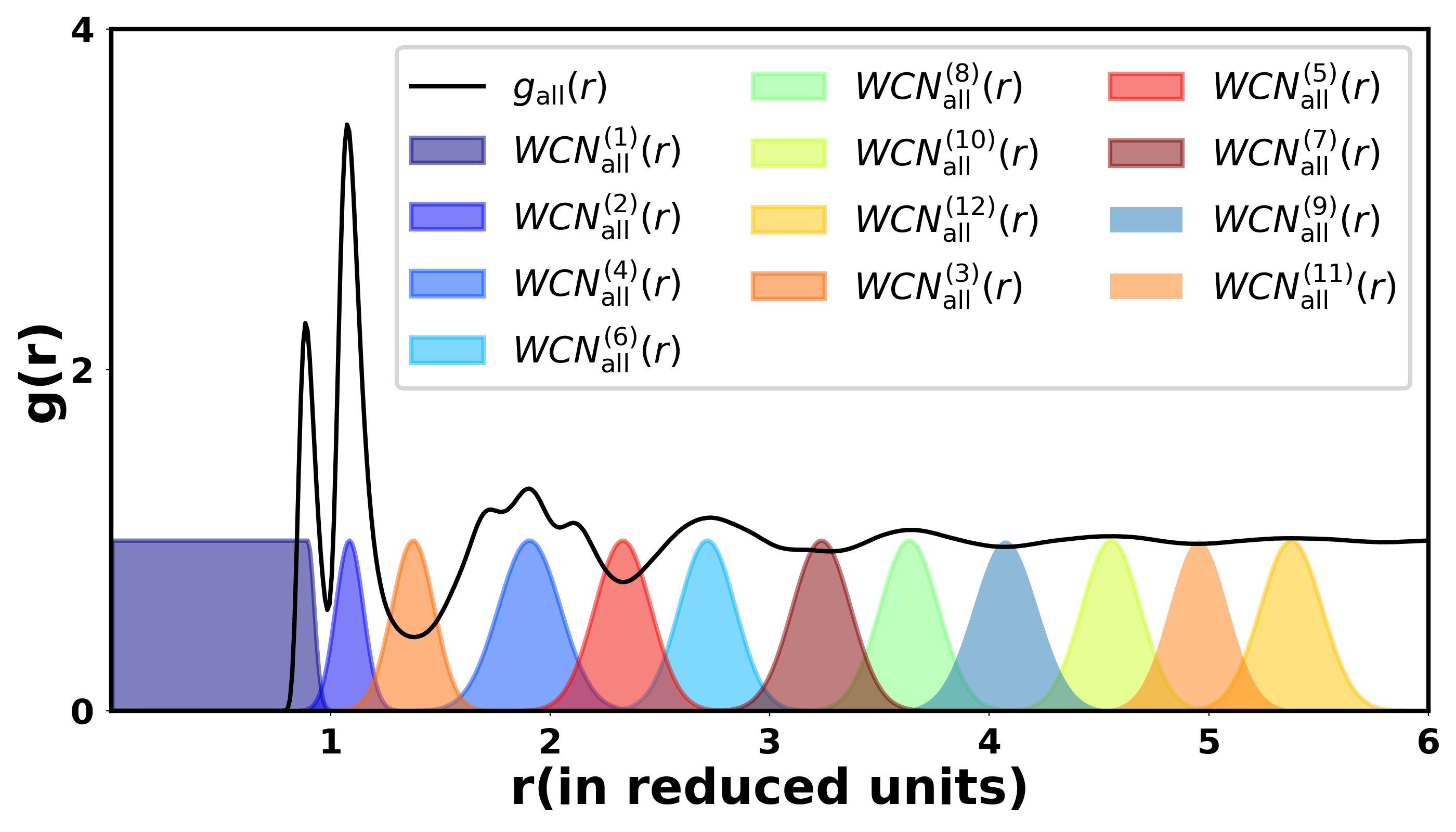
Using molecular dynamics simulations of this model system, the CN of a particle can be calculated. In this study, the A/B identity of the particles is ignored, which can be thought as the supercooled liquid state being generated from an effective one-component system. However, CN-based features suffer a strict cut-off value to determine whether a neighbor particle is counted as in or out of the shell. To avoid this hard assignment, weighted coordination numbers (WCNs) Rudzinski et al. (2019), which utilize the normalized Gaussian distribution based on the shell structure of the system g(r)(1(a)) to weight the contribution of each neighboring particle based on the particle’s distance to the center one. Using the relevant solvation shell features as identified maxima and minima along the radial distribution function, the normalized Gaussian distribution functions are placed at the center of these shell features as shown in 1(a). The width of the Gaussian functions depends on the area that the solvation feature covers and neighboring Gaussians such that the value of the intersection is assigned to 0 or roughly 0.25 depending on whether or not the two shells are largely overlapping. However, width and the size of the overlapping areas of the Gaussians do not change the consistency of the final results. The WCNs smooth out transitions between solvation shells by counting the particles sitting at the center of the features as one while the one further away from the center feature is counted as a fraction based on the Gaussian distribution function. For each configuration, employing this WCN implementation, each component of a particle’s WCNs vector is determined by summing the weight from all surrounding particles within that shell and the dimension of the WCN vector is determined by the number of shells reasonably covering the main features of the g(r), $N=12$ in 1(a); other numbers of shells tested yield consistent results.

For a single configuration of the simulation, WCNs of all particles are collected from the particles’ coordination numbers smoothed using the g(r), hence the features data for the entire system is represented by a matrix ${\widetilde{\bf X}}$ of MxN which is obtained from N WCNs for each of M particles system. WCNs are noisy and complicated in a disordered system, hence require a further step to remove some of these noises. Instead of WCNs, averaged WCNs is used which has a form: $\overline{WCN}_{i}=\frac{1}{N_{b}}{\sum_{j}^{N_{b}}WCN_{j}}$, where $N_{b}$ is the number of neighboring particles in each shell plus the particle $i$ itself.

For each particle, each of $N$ features in the $\overline{WCNs}$ matrix is constructed separately to describe its own local solvation shell environment with respect to its surrounding particles, it is disconnected from each other to form a proper feature space. To resolve this issue, Principal Component Analysis (PCA)  Shlens (2014) is used for dimension reduction, namely to linearly transform original $\overline{WCNs}$ matrix into a new feature space that reduce $N$ particles’ features to a few correlated ones. Mathematically, PCA can be done through the following three steps:

• •

  Obtaining the mean-free data $\mathbb{X=\widetilde{X}-\langle\widetilde{X}\rangle}$ where the average is over ${M}$ particles for each component of WCNs.

• •

  Forming the correlation matrix $\mathbb{C=X^{\intercal}X}$, which is $N\times N$.

• •

  The principle components $\mathbb{u_{i}}$ are obtained after solving the eigenvalue problem: $\mathbb{Cu_{i}={\bm{\sigma_{i}}}^{2}u_{i}}$. The eigenvalue $\mathbb{\bm{\sigma_{i}^{2}}}$ measures the variance of the data along each principle component(PC) $i$. PCA is optimal in term of seeking small numbers of PCs but maximizing cumulative proportion of variance explained (PVE) $\mathbb{\bm{\sigma_{i}^{2}}}$ by each principle component. In other words, the numbers of retained PCs depend on their total PVE such that the total PVE is $\geq$ 95$\%$ of total variances presented in ${\widetilde{\bf X}}$.

The new complete basis composes of all PCs: $\mathbb{U=[u_{1},u_{2},..u_{N}]}$ where each $\mathbb{u_{i}}$ is a collective coordinate with $N$ components corresponding to the number of features in the data input. In our study, the first three PCs retains about 85-90%, so 6-7 PCs are sufficient enough to form PC’s basis whose PVE could be $\geq$ 95$\%$ of total variances presented in ${\widetilde{\bf X}}$. The new coordinates (PC representation) are generated from an inner product of original $\overline{WCNs}$ matrix with the PC’s basis (PC-space), mathematically, $\mathbb{Y=U^{\intercal}\widetilde{\bf X}}$. We then use K-means clustering method to decipher hidden structures of the PC representation by classifying particles into distinct clusters called meso-states. K-means clustering is chosen because it is an unsupervised standard technique that geometrically separate particles into clusters that aggregated together because of certain similarities.

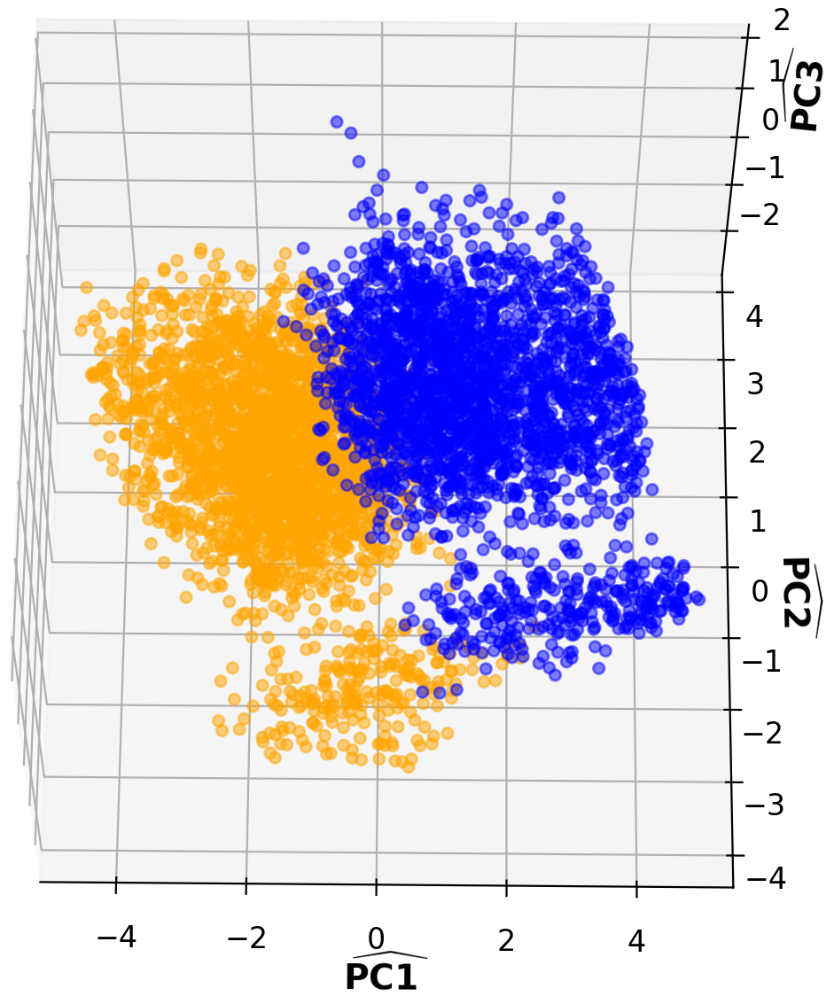
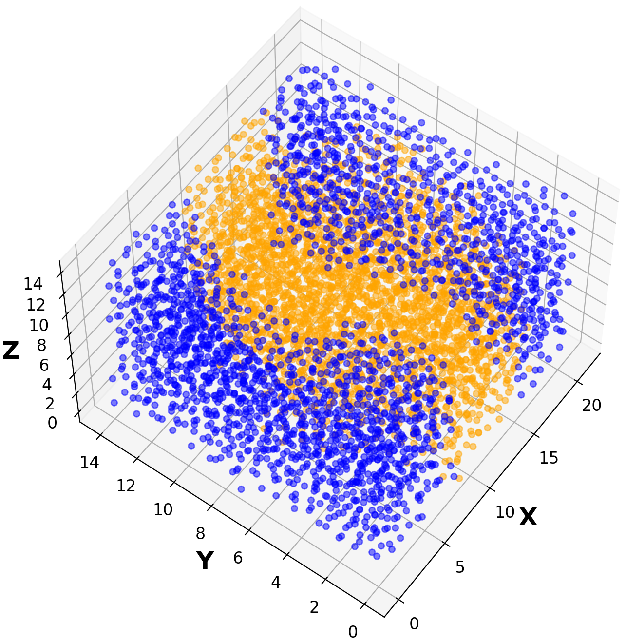
However, the K-means requires prior knowledge of the number of existing clusters K in the data structure to work effectively, which is generally unknown in most cases. An implementation of the Elbow convergent test could provides a reasonable prediction of the K values. The Elbow test permits the number of clusters K being varied freely and computes the Within-Cluster Sum of Square Distance (Wss) which is the sum of square distances between each data point and the centroid within a cluster. As the number of clusters K increase, the Wss will start to decrease and eventually become roughly constant regardless of further increasing K. The Elbow plot of the Wss against K looks like an Elbow shape where the Elbow point normally corresponds to an initial guess of K used in K-means clustering. In many cases, the Elbow plot has a clear Elbow point which indicates a good guess for K-means. In our case, initial K remains uncertain because the Elbow shape is poor to single out an Elbow point, thus we can only narrow down a possible range of K values (K = 2 to 5) (2(c)). After a careful trial-and-error process with help of the co-learning strategy, K = 2 is selected; details of the process is discussed in the Appendix A. Given K = 2, particles in the PC-space are classified into 2 distinct meso-states (2(a)), then a direct mapping using the identities of particles in each meso-state in the PC-space also forms aggregated clusters in the configurational space as shown in 2(b); different projected angles of 2(a) and 2(b) to confirm the clustering structures both in PC and real space are in Appendix B. Naturally, each meso-state have mixing A and B particles. On the other hand, each type of (A or B) particles itself appears as two distinct aggregated domains in the configurational space. This is clearly demonstrated in the Appendix C.

Although domains are generated in the real space by a simple mapping of particles’ identities in the PC-space after K-means clustering, there are two issues needed to be addressed. Firstly, the principle of K-means clustering relies on assigning a particle to a cluster where its Euclidean distance (E-dist) to the centroid of that cluster is the closest among others. In other words, assignment of a particle depends on the E-dist measure sensitively which becomes robust for core particles of each meso-state because the difference of their distances from one state to another is well-defined. However, the E-dist criterion becomes an issue to assign interfacial particles due to the small differences in their distances to either states, so it could lead to misclassification. Secondly, even though identities of clusters are preserved from the PC-space to the configurational space the inverse transfer of the knowledge is not clear, but physically the transfer of knowledge should be bi-directional. Thus, a co-learning strategy is developed as the following:

1. 1.

   Perform K-means clustering in the PC-space.

2. 2.

   Use the initial knowledge of the clustering from the PC-space to perform a Gaussian Mixture (GM) classification in the configurational space to soften the hard assignment from the K-means:

   1. (a)

      do a direct mapping of particles identities in the PC space to identify distinct nano-domains in the real space.

   2. (b)

      build a mixture model of multivariate Gaussian distributions of domains, then assignment of a particle belonging to a domain is determined by maximizing Gaussian probability among different domains.

3. 3.

   Similar to step 2, perform GM in the PC-space from the clustering knowledge in the configurational space.

4. 4.

   Iteratively perform GM classification in both spaces until convergence.

Classification of interfacial particles by the co-learning strategy converges quickly in both PC-space(3(a),3(c)) and configurational space (3(b),3(d)) after few iterations (3-5 runs on average) as shown in the Fig. 3. The co-learning strategy shows improvement over K-means as it generalizes and fills the missing information from a direct information transfer from the PC-space to the configurational space. In other words, it allows a bi-directional information transfer. Firstly, correct classification of interfacial particles comes from using probabilistic clustering like GM to avoid sensitivities of E-dist criterion of the K-means. This GM clustering allows assignment of interfacial particles to two states and the decision is made by the maximum-likelihood of the Gaussian probability, which creates a boundary region of meso-states in the PC-space as shown in 3(c). In the configurational space, we also find that the core particles in both domains are still the same, only interfacial particles are properly re-assigned to make the final results consistent with the direct mapping (2(b)) and co-learning strategy (3(d)). Secondly, the classification scheme utilizes the information from both spaces in a self-consistent manner.

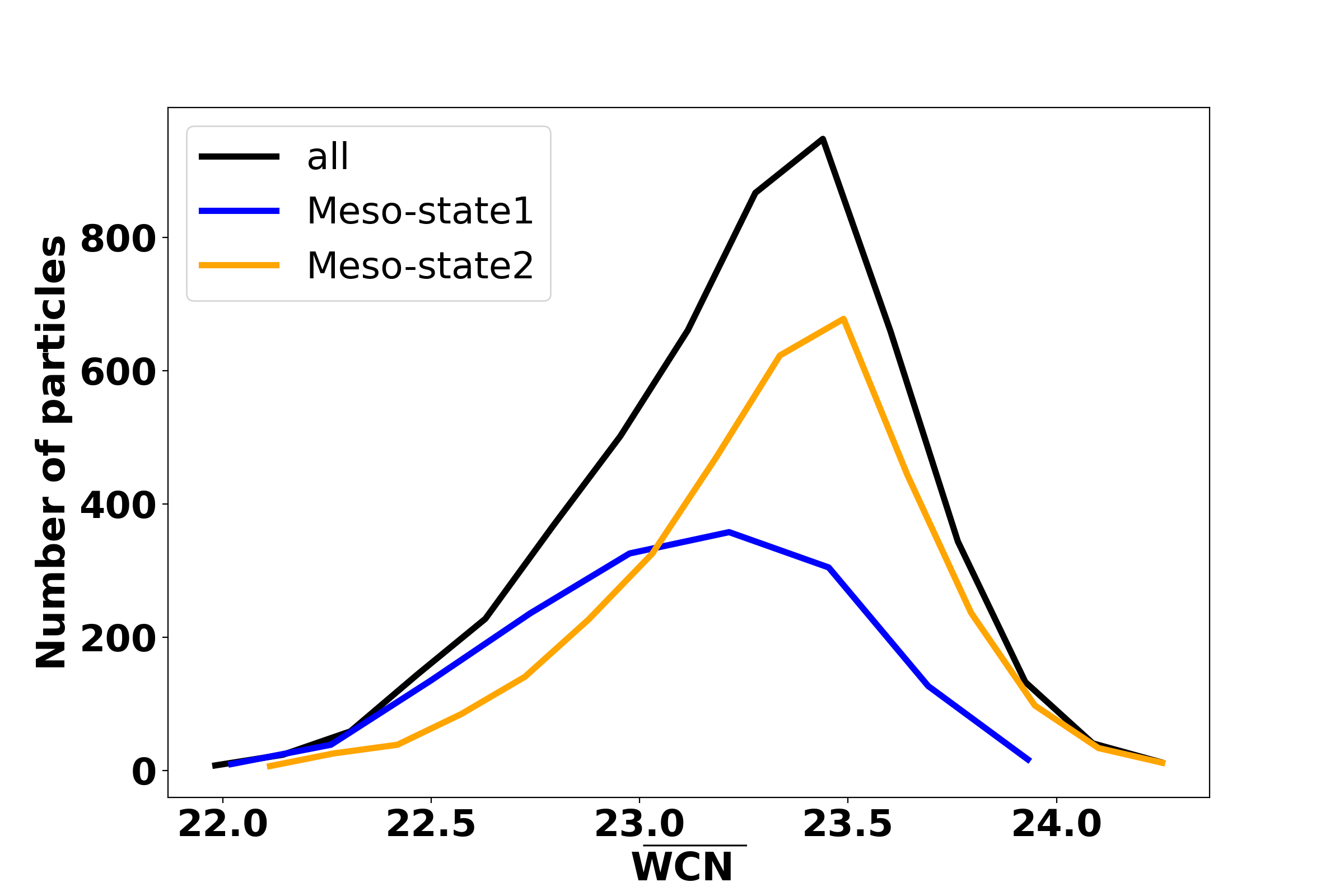
In the previous section, a picture of structural and configurational heterogeneity is revealed by the classification of the system into meso-states (in PC-space) or nano-domains (in real space). In order to clarify the physical interpretation of these nano-domains, it is observed that in the PC-space bimodality of $\overline{WCNs}$ distribution along each solvation shell. Fig. 4b-f provide clear evidence of two meso-states in the PC space, for example the total $\overline{WCNs}$ distributions along first five solvation shells of the system are decomposed into distributions of each individual meso-state as there is a co-existence of two meso-states with different unique local structures. Furthermore, the bimodal distributions of the $\overline{WCNs}$ along all shells in the PC-space can be transformed into a construction of partial g(r)s in the configurational space as shown in 4(a). The total $\it g(r)$ of the whole system is the summation of the weighted partial $\it g(r)$s (blue and orange curves) representing two meso-states. In other words, the classification scheme provides a method to decompose the total $\it g(r)$ of the system into two partial $\it g(r)$s, which represent two different meso-structures whose particles form various domains that tile up the whole configurational space.

Another quantitative measure of these distinct meso-states is to compute density and pressure profiles of the domains. Because the shapes of the domains are irregular, the thermodynamic properties of the two meso-states were calculated using a spherical region inside a domain of meso-state 1 and a thin shell in the outermost meso-state 2 region. 5(a) shows the radial distribution of the atomic number density from the center of meso-state 1. Meanwhile, the six components of the pressure tensor ($\it p_{xx}$, $\it p_{yy}$, $\it p_{zz}$, $\it p_{xy}$,$\it p_{yx}$,$\it p_{xz}$ and $\it p_{zx}$) for each atom are computed in the Cartesian coordinate. The pressure tensor is then transformed into polar coordinate representation whose corresponding components will be ($\it p_{rr}$, $\it p_{\theta\theta}$, $\it p_{\phi\phi}$, $\it p_{r\theta}$, $\it p_{\theta\phi}$ and $\it p_{\phi r}$). It is noted that the magnitude of the off-diagonal terms is negligible compared to diagonal terms, thus the pressure tensor can be expressed as  Gunawardana and Song (2018); Rowlinson and Widom (2013):

where $\textbf{e}_{r}$, $\textbf{e}_{\theta}$ and $\textbf{e}_{\phi}$ are unit vectors, $\it P_{N}$ and $\it P_{T}$ are the radial or normal and transverse components of the pressure tensor, respectively. The radial profiles of the components $\it P_{N}(r)$ and $\it P_{T}(r)$ are obtained by integrating out the angular degrees of freedom over thin spherical shells extending outwards from the origin. 5(b) shows the normal ($\it P_{N}$) and tangential ($\it P_{T}$) pressure profiles approximated as a spherical interface within the solid angle of the calculation. It is verified that the normal and tangential profiles statisfy the mechanical equilibrium,$\bm{\nabla}\cdot\bm{P}=0$, which in spherical coordinates is given by Ballal et al. (2019); Rowlinson and Widom (2013):

where the second term is the derivative of the normal pressure with respect to distance from the center of meso-state 1.

The formation of local spherical interfaces from density and pressure profiles in Fig. 5 signifies a strong indication for the co-existence of two local distinct meso-states in supercooled states.

With our classification scheme, the bimodal decomposition of the g(r), the density and pressure profiles seem to indicate an coexistence of two phases with domain structures after quenching, where similar liquid-liquid phase separation is also observed in a model 2D system with such classification scheme Nguyen and Song (2023). To further check the validity of such a picture, some dynamical signatures of a liquid-liquid phase separation are evaluated.

First of all, there will be two well separated relaxation time scales in such a scenario. The particles within the domains that belong to the same meso-states should have the same diffusion behavior as they are in the same thermodynamic state. After finding the nano-domains in the configurational space, core particles, the particles stay in that domain during the whole simulation time, in each domain are sorted. Core particles are colored as red and grey for meso-state 1 (blue) and black and green for meso-state 2 (orange) as shown in Fig. 6a,b. 2D cross section of core particles is taken for the purpose of visualization. Collected core particles from each domain are then used to compute mean-square displacements to get diffusion constant by Einstein relation. Fig. 6c,d show different diffusion constant distribution of different domains at different temperatures, hence supports the picture that the domains that belong to the same meso-state have the same diffusion behavior.

In the Section II.2, the stability of nano-domains is associated with the onset of cage-breaking processes which is reflected as a plateau in the self intermediate coherent function $F(k,t)$ or in diffusion dynamics via MSD(1(b)). The timescale of the cage processes depends on temperature, a quantitative study will interesting, but some qualitative observations can still be made. Given the glass transition temperature being $T_{g}^{*}$ = 0.25 for this system, different configurational snapshots can be used to qualitatively examine timescale of nano-domains. Fig. 7 shows three different 10ns lag time snapshots which are taken at three different temperatures. At $T^{*}$ = 0.2 which is below $T_{g}^{*}$, almost all of particles are immobile and freeze at their local domains, so lifetime of nano-domains are indefinitely long. Meanwhile, as temperature goes up, more particles are able to escape out the cage as illustrated from $T^{*}$ = 0.3 to $T^{*}$ = 0.37 in Fig. 7, hence nano-domain shapes are changing relatively quickly and become less static. These phenomena are confirmed by quantitatively evaluating particles fluctuation of the domains as shown in Fig. 8a-c. The magnitude of particles fluctuations increases as the temperature increases because of higher number of mobile particles.

Another signature of the liquid-liquid phase separation that follows the quenching from a high temperature equilibrium (normal liquid) state to a super-cooled state is the scaling law of the domain size growth Aranson (2011); Binder (1975); Humayun and Bray (1991). In this case, the two meso-states are the equilibrium thermodynamic states with domains formed either via spinodal decomposition or nucleation such as shown in 3(d) Nguyen and Song (2023); Brickley et al. (2023). It is well-established that the growth of characteristic domain size follows an algebraic growth law in time  Aranson (2011); Binder (1975); Humayun and Bray (1991) $L(t)\sim t^{1/3}$ for conserved scalar order parameters (even though the A/B particles are treated as the same in our classficaiton, but the growth dynamics still follows the conserved order parameter scaling law as the real dynamics is still constrained by the swapping of A/B identity)  Bray et al. (1991); Mazenko (1990); Mazenko et al. (1988); Liu and Mazenko (1991); Bray (1990) which can be tested by the calculation of equal-time correlation function $C(r,t)$ from our classification. Considering a scalar order parameter $\psi$, the equal-time correlation is: $C(r,t)=N^{-1}\sum_{i}\psi_{i}(t)\psi_{i+r}(t)$ where N is the number of particles, $i+r$ indicates a neighboring particle displaced by a distance $r$ relative to the reference particle $i$ with $\psi_{i}$ = +1 for particles identities of state 1 and $\psi_{i}$ = -1 for particles identities of state 2, hence the product of $\psi_{i}(t)\psi_{i+r}(t)$ will be +1 between pair of particles from the same state and will be -1 otherwise. Since the domain identities for each particle are known from the classification scheme, the result of $C(r,t)$ indeed confirms the scaling law of domains growth $L(t)\sim t^{1/3}$ as shown in 8(d).

Finally, similar to the 2D case Nguyen and Song (2023), the number of domains belonging to the same meso-state will increase to tile up the whole system as the system size increases. However, 3D domains are hard to visualize, so their spatial structures are illustrated by taking different 2D cross sections at different configurations. 9(a) and 9(c) shows two different cross sections of two domains that belong to the same meso-state1. These two domains are also shown by taking a second snapshot at 2ns later in 9(b) and 9(c). As the system size continues to increase, the meso-state1 will split into more domains as shown in Fig. 10 for 50000 particles system. It should be emphasized that the structure of a domain might disappear in some regions of the space along different cross sections as happened to the bifurcated domain 2,3,4 to illustrate the finiteness of each domain in 3D configurational space.

References

- Crowe et al. (1998) J. H. Crowe, J. F. Carpenter, and L. M. Crowe, Annual Review of Physiology 60, 73 (1998), pMID: 9558455, https://doi.org/10.1146/annurev.physiol.60.1.73 .
- Debenedetti et al. (2001) P. G. Debenedetti, T. M. Truskett, C. P. Lewis, and F. H. Stillinger (Academic Press, 2001) pp. 21–79.
- Sastry et al. (1998) S. Sastry, P. G. Debenedetti, and F. H. Stillinger, Nature 393, 554 (1998).
- Andersen (2005) H. C. Andersen, Proceedings of the National Academy of Sciences 102, 6686 (2005), https://www.pnas.org/doi/pdf/10.1073/pnas.0500946102 .
- Kob et al. (1997) W. Kob, C. Donati, S. J. Plimpton, P. H. Poole, and S. C. Glotzer, Physical Review Letters 79, 2827 (1997).
- Gotze and Sjogren (1992) W. Gotze and L. Sjogren, Reports on Progress in Physics 55, 241 (1992).
- Cubuk et al. (2015) E. D. Cubuk, S. S. Schoenholz, J. M. Rieser, B. D. Malone, J. Rottler, D. J. Durian, E. Kaxiras, and A. J. Liu, Physical Review Letters 114, 108001 (2015).
- Stillinger (1995) F. H. Stillinger, SCIENCE 267, 1935 (1995).
- Smessaert and Rottler (2013) A. Smessaert and J. Rottler, Physical Review E 88, 022314 (2013).
- Candelier et al. (2010) R. Candelier, A. Widmer-Cooper, J. K. Kummerfeld, O. Dauchot, G. Biroli, P. Harrowell, and D. R. Reichman, Physical Review Letters 105, 135702 (2010).
- Kawasaki and Tanaka (2014) T. Kawasaki and H. Tanaka, Physical Review E 89, 062315 (2014).
- Yang et al. (2016) X. Yang, R. Liu, M. Yang, and K. Chen, Physical Review Letters 116 (2016), 10.1103/PhysRevLett.116.238003.
- Doliwa and Heuer (1998) B. Doliwa and A. Heuer, Physical Review Letters 80, 4915 (1998).
- Glotzer (2000) S. C. Glotzer, Journal of Non-Crystalline Solids 274, 342 (2000), physics of Non-Crystalline Solids 9.
- Sillescu (1999) H. Sillescu, Journal of Non-Crystalline Solids 243, 81 (1999).
- Ediger (2000) M. D. Ediger, Annual Review of Physical Chemistry 51, 99 (2000), pMID: 11031277, https://doi.org/10.1146/annurev.physchem.51.1.99 .
- Royall and Williams (2015) C. P. Royall and S. R. Williams, Physics Reports 560, 1 (2015), the role of local structure in dynamical arrest.
- Cavagna (2009) A. Cavagna, Physics Reports 476, 51 (2009).
- Donati et al. (1998) C. Donati, J. F. Douglas, W. Kob, S. J. Plimpton, P. H. Poole, and S. C. Glotzer, Physical Review Letters 80, 2338 (1998).
- Adam and Gibbs (1965) G. Adam and J. H. Gibbs, The Journal of Chemical Physics 43, 139 (1965), https://doi.org/10.1063/1.1696442 .
- Vidal Russell and Israeloff (2000) E. Vidal Russell and N. E. Israeloff, Nature 408, 695 (2000).
- Ludovic et al. (2006) B. Ludovic, B. Giulio, B. Jean-Philippe, C. Luca, M. Djamel, L. Denis, L. F., and P. Matteo, Science (New York, N.Y.) 310, 1797 (2006).
- Kirkpatrick et al. (1989) T. R. Kirkpatrick, D. Thirumalai, and P. G. Wolynes, Physical Review A 40, 1045 (1989).
- Viot et al. (2000) P. Viot, G. Tarjus, and D. Kivelson, The Journal of Chemical Physics 112, 10368 (2000), https://doi.org/10.1063/1.481674 .
- Garrahan and Chandler (2002) J. P. Garrahan and D. Chandler, Physical Review Letters 89, 035704 (2002).
- Hurley and Harrowell (1995) M. M. Hurley and P. Harrowell, Physical Review E 52, 1694 (1995).
- Bennemann et al. (1999) C. Bennemann, C. Donati, J. Baschnagel, and S. C. Glotzer, Nature 399, 246 (1999).
- Donati et al. (2002) C. Donati, S. Franz, S. C. Glotzer, and G. Parisi, Journal of Non-Crystalline Solids 307-310, 215 (2002).
- Whitelam et al. (2004) S. Whitelam, L. Berthier, and J. P. Garrahan, Physical Review Letters 92, 185705 (2004).
- Berthier (2004) L. Berthier, Physical Review E 69, 020201 (2004).
- Goldstein (1969) M. Goldstein, The Journal of Chemical Physics 51, 3728 (1969), https://doi.org/10.1063/1.1672587 .
- Berthier and Biroli (2011) L. Berthier and G. Biroli, Reviews of Modern Physics 83, 587 (2011).
- Gibbs and DiMarzio (1958) J. H. Gibbs and E. A. DiMarzio, The Journal of Chemical Physics 28, 373 (1958), https://doi.org/10.1063/1.1744141 .
- Bouchaud and Biroli (2004) J.-P. Bouchaud and G. Biroli, Journal of Chemical Physics 121, 7347 (2004), cited by: 333; All Open Access, Green Open Access.
- BERNAL (1959) J. D. BERNAL, Nature 183, 141 (1959).
- BERNAL (1960) J. D. BERNAL, Nature 185, 68 (1960).
- Finney (1970) J. Finney, Proceedings of the Royal Society A: Mathematical, Physical and Engineering Sciences 319 (1970), cited by: 299.
- Anikeenko and Medvedev (2007) A. V. Anikeenko and N. N. Medvedev, Physical Review Letters 98, 235504 (2007).
- Anikeenko et al. (2008) A. V. Anikeenko, N. N. Medvedev, and T. Aste, Physical Review E 77, 031101 (2008).
- Steinhardt et al. (1983) P. J. Steinhardt, D. R. Nelson, and M. Ronchetti, Physical Review B 28, 784 (1983).
- Lechner and Dellago (2008) W. Lechner and C. Dellago, The Journal of Chemical Physics 129, 114707 (2008), https://doi.org/10.1063/1.2977970 .
- Tsuzuki et al. (2007) H. Tsuzuki, P. S. Branicio, and J. P. Rino, Computer Physics Communications 177, 518 (2007).
- Faken and Jónsson (1994) D. Faken and H. Jónsson, Computational Materials Science 2, 279 (1994).
- Honeycutt and Andersen (1987) J. D. Honeycutt and H. C. Andersen, The Journal of Physical Chemistry 91, 4950 (1987), https://doi.org/10.1021/j100303a014 .
- Williams (2007) S. R. Williams, arXiv: Soft Condensed Matter (2007).
- Malins et al. (2013) A. Malins, S. R. Williams, J. Eggers, and C. P. Royall, The Journal of Chemical Physics 139, 234506 (2013), https://doi.org/10.1063/1.4832897 .
- Dunleavy et al. (2015) A. J. Dunleavy, K. Wiesner, R. Yamamoto, and C. P. Royall, Nature Communications 6, 6089 (2015).
- Shannon (1948) C. E. Shannon, The Bell System Technical Journal 27, 379 (1948).
- Dunleavy et al. (2012) A. J. Dunleavy, K. Wiesner, and C. P. Royall, Physical Review E 86, 041505 (2012).
- Ronhovde et al. (2012) P. Ronhovde, S. Chakrabarty, D. Hu, M. Sahu, K. K. Sahu, K. F. Kelton, N. A. Mauro, and Z. Nussinov, Scientific Reports 2, 329 (2012).
- James et al. (2014) G. James, D. Witten, T. Hastie, and R. Tibshirani, An introduction to Statistical Learning with Application in R, Springer Texts in Statistics (Springer, 2014).
- Scherer et al. (2015) M. K. Scherer, B. Trendelkamp-Schroer, F. Paul, G. Pérez-Hernández, M. Hoffmann, N. Plattner, C. Wehmeyer, J.-H. Prinz, and F. Noé, Journal of Chemical Theory and Computation, Journal of Chemical Theory and Computation 11, 5525 (2015).
- M. (2006) B. C. M., Pattern recognition and machine learning (Springer, 2006).
- Murphy (2012) K. P. Murphy, Machine Learning: A Probabilistic Perspective (The MIT Press, 2012).
- Kob and Andersen (1995) W. Kob and H. C. Andersen, Physical Review E 51, 4626 (1995).
- Kob and Andersen (1994) W. Kob and H. C. Andersen, Physical Review Letters 73, 1376 (1994).
- Middleton and Wales (2001) T. F. Middleton and D. J. Wales, Physical Review B 64, 024205 (2001).
- Thompson et al. (2022) A. P. Thompson, H. M. Aktulga, R. Berger, D. S. Bolintineanu, W. M. Brown, P. S. Crozier, P. J. in ’t Veld, A. Kohlmeyer, S. G. Moore, T. D. Nguyen, R. Shan, M. J. Stevens, J. Tranchida, C. Trott, and S. J. Plimpton, Computer Physics Communications 271, 108171 (2022).
- Montero de Hijes et al. (2020) P. Montero de Hijes, J. R. Espinosa, V. Bianco, E. Sanz, and C. Vega, The Journal of Physical Chemistry C, The Journal of Physical Chemistry C 124, 8795 (2020).
- Bai and Li (2006) X.-M. Bai and M. Li, The Journal of Chemical Physics 124, 124707 (2006), https://doi.org/10.1063/1.2184315 .
- Janssen (2018) L. M. C. Janssen, Frontiers in Physics 6 (2018), 10.3389/fphy.2018.00097.
- Schrøder and Dyre (2020) T. B. Schrøder and J. C. Dyre, The Journal of Chemical Physics 152, 141101 (2020), https://doi.org/10.1063/5.0004093 .
- Rudzinski et al. (2019) J. F. Rudzinski, M. Radu, and T. Bereau, The Journal of Chemical Physics 150, 024102 (2019), https://doi.org/10.1063/1.5064808 .
- Shlens (2014) J. Shlens, Educational 51 (2014).
- Gunawardana and Song (2018) K. G. S. H. Gunawardana and X. Song, The Journal of Chemical Physics 148, 204506 (2018), https://doi.org/10.1063/1.5021944 .
- Rowlinson and Widom (2013) J. S. Rowlinson and B. Widom, Molecular theory of capillarity (Courier Corporation, 2013).
- Ballal et al. (2019) D. Ballal, Q. Lu, M. Raju, and X. Song, The Journal of Chemical Physics 151, 134108 (2019), https://doi.org/10.1063/1.5116252 .
- Nguyen and Song (2023) V. Nguyen and X. Song, Journal of Physics: Condensed Matter (submitted, 2023), 10.48550/arXiv.2301.05990.
- Aranson (2011) I. Aranson, Journal of Statistical Physics 142, 220 (2011).
- Binder (1975) K. Binder, “Dynamics of first order phase transitions,” in Fluctuations, Instabilities, and Phase Transitions, edited by T. Riste (Springer US, Boston, MA, 1975) pp. 53–86.
- Humayun and Bray (1991) K. Humayun and A. J. Bray, J. Phys. A: Math. Gen. 24 (1991), 10.1088/0305-4470/24/8/030.
- Brickley et al. (2023) J. Brickley, V. Nguyen, and X. Song, “unpublished results,” (2023).
- Bray et al. (1991) A. J. Bray, K. Humayun, , and T. J. Newman, Phys. Rev. B 43, 3699 (1991).
- Mazenko (1990) G. F. Mazenko, Physical Review B 42, 4487 (1990).
- Mazenko et al. (1988) G. F. Mazenko, O. T. Valls, and M. Zannetti, Physical Review B 38, 520 (1988).
- Liu and Mazenko (1991) F. Liu and G. F. Mazenko, Phys. Rev. B 44, 9185 (1991).
- Bray (1990) A. J. Bray, Phys. Rev. B 41, 6724 (1990).