AutoDRIVE: A Comprehensive, Flexible and Integrated Digital Twin Ecosystem for Enhancing Autonomous Driving Research and Education
Abstract
Prototyping and validating hardware-software components, sub-systems and systems within the intelligent transportation system-of-systems framework requires a modular yet flexible and open-access ecosystem. This work presents our attempt towards developing such a comprehensive research and education ecosystem, called AutoDRIVE, for synergistically prototyping, simulating and deploying cyber-physical solutions pertaining to autonomous driving as well as smart city management. AutoDRIVE features both software as well as hardware-in-the-loop testing interfaces with openly accessible scaled vehicle and infrastructure components. The ecosystem is compatible with a variety of development frameworks, and supports both single and multi-agent paradigms through local as well as distributed computing. Most critically, AutoDRIVE is intended to be modularly expandable to explore emergent technologies, and this work highlights various complementary features and capabilities of the proposed ecosystem by demonstrating four such deployment use-cases: (i) autonomous parking using probabilistic robotics approach for mapping, localization, path planning and control; (ii) behavioral cloning using computer vision and deep imitation learning; (iii) intersection traversal using vehicle-to-vehicle communication and deep reinforcement learning; and (iv) smart city management using vehicle-to-infrastructure communication and internet-of-things.
Index Terms:
Education Robotics; Hardware-Software Integration in Robotics; Intelligent Transportation Systems; Product Design, Development and PrototypingI Introduction
Advancing the field of connected autonomous vehicles (CAVs) [1] requires scientific and technological research in conjunction with comprehensive education of methods and tools to overcome existing challenges and prepare the next generation of practitioners.
Inasmuch as meaningful verification and validation (V&V) efforts demand end-to-end stress testing across scales at component/sub-system/system levels, there is a great incentive for exploring the creation and exploitation of varying grades of virtual (simulation-based) and physical (hardware-in-the-loop) testing platforms to alleviate the monetary, spatial, temporal and safety constraints associated with rapid-prototyping of CAV solutions. In a research setting, such platforms can accelerate the process of designing experiments, recording datasets as well as re-iteratively prototyping and validating autonomy solutions. In an educational setting, such platforms can aid in designing interactive demonstrations, hands-on assignments, projects, and competitions.
However, existing platforms for this purpose are observed to limit the throughput of developing and validating connected autonomy solutions. Firstly, most of these platforms lack the integrity required to promote hardware-software co-development; some only offer software simulation tools (e.g., [2, 3, 4]), while others only provide scaled physical vehicles (e.g., [5, 6, 7, 8]) to test autonomy algorithms. Such isolated platforms not only decelerate the prototyping phase due to compatibility issues, but also adversely affect the validation phase involving simulation to real-world (sim2real) deployments. Secondly, most of these platforms focus specifically on vehicles rather than a holistic intelligent transportation ecosystem involving infrastructure, traffic elements and peer agents, which limits their applications. Thirdly, some of these platforms (e.g., [9, 10]) are domain specific with limited sensing modalities, stringent design requirements and/or fixed development frameworks; some (e.g. [11]) even lack a high-level computation unit and are merely teleoperated from a remote server to execute the intended mission.
| Platform/Ecosystem |
|
|
|
Cost∗ | Sensing Modalities | Computational Resources |
|
Dedicated Simulator | V2X Support | API Support | ||||||||||||||||||
|
Scale |
Open Hardware |
Open Software |
Throttle |
Steering |
Wheel Encoders |
GPS/IPS |
IMU |
LIDAR |
Camera |
High-Level | Low-Level |
|
|
Multi-Agent Support |
V2V | V2I |
C++ |
Python |
ROS |
MATLAB/Simulink |
Webapp |
|||||||
| AutoDRIVE | 1:14 | ✓ | ✓ | $450 | ✓ | ✓ | ✓ | ✓ | ✓ | ✓ | ✓ | Jetson Nano | Arduino Nano | ✓ | ★ | ✓ | ✓ | ✓ | ✓ | ✓ | ✓ | ✓ | ★ | ✓ | ||||
| MIT Racecar | 1:10 | ★ | ✓ | $2,600 | ✗ | ✗ | ✗ | ✗ | ✓ | ✓ | ✓ | Jetson TX2 | VESC | ✓ | ✗ | Gazebo | ★ | ★ | ✗ | ✗ | ✗ | ✓ | ✗ | ✗ | ||||
| AutoRally | 1:5 | ★ | ✓ | $23,300 | ✗ | ✗ | ✓ | ✓ | ✓ | ✓ | ✓ | Custom | Teensy LC/Arduino Micro | ✓ | ✗ | Gazebo | ★ | ★ | ✗ | ✗ | ✗ | ✓ | ✗ | ✗ | ||||
| F1TENTH | 1:10 | ★ | ✓ | $3,260 | ✗ | ✗ | ✗ | ✗ | ✗ | ✓ | ✗ | Jetson TX2 | VESC 6MkV | ✓ | ✗ | RViz/Gazebo | ✓ | ✓ | ✗ | ✗ | ✗ | ✓ | ✗ | ✗ | ||||
| DSV | 1:10 | ★ | ✓ | $1,000 | ✗ | ✗ | ✓ | ✗ | ✓ | ✓ | ✓ | ODROID-XU4 | Arduino (Mega + Uno) | ✓ | ✗ | ✗ | ✗ | ✗ | ✗ | ✗ | ✗ | ✓ | ✗ | ✗ | ||||
| MuSHR | 1:10 | ★ | ✓ | $930 | ✗ | ✗ | ✗ | ✗ | ✗ | ✗ | ✓ | Jetson Nano | Turnigy SK8-ESC | ✓ | ✗ | RViz | ✓ | ✓ | ✗ | ✗ | ✗ | ✓ | ✗ | ✗ | ||||
| HyphaROS RaceCar | 1:10 | ★ | ✓ | $600 | ✗ | ✗ | ✗ | ✗ | ✓ | ✓ | ✗ | ODROID-XU4 | RC ESC TBLE-02S | ✓ | ✗ | ✗ | ✗ | ✗ | ✗ | ✗ | ✗ | ✓ | ✗ | ✗ | ||||
| Donkey Car | 1:16 | ★ | ✓ | $370 | ✗ | ✗ | ✗ | ✗ | ✗ | ✗ | ✓ | Raspberry Pi | ESC | ✓ | ✗ | Gym | ✗ | ✗ | ✗ | ✗ | ✓ | ✗ | ✗ | ✗ | ||||
| BARC | 1:10 | ★ | ✓ | $1,030 | ✗ | ✗ | ✓ | ✗ | ✓ | ✗ | ✓ | ODROID-XU4 | Arduino Nano | ✓ | ✗ | ✗ | ✗ | ✗ | ✗ | ✗ | ✗ | ✓ | ✗ | ✗ | ||||
| OCRA | 1:43 | ★ | ✓ | $960 | ✗ | ✗ | ✗ | ✗ | ✓ | ✗ | ✗ | None | ARM Cortex M4 C | ✓ | ✗ | ✗ | ✓ | ✗ | ✗ | ✓ | ✗ | ✗ | ✓ | ✗ | ||||
| QCar | 1:10 | ✗ | ✗ | $20,000 | ✗ | ✗ | ✓ | ✗ | ✓ | ✓ | ✓ | Jetson TX2 | Proprietary | ✓ | ✗ | Simulink | ✓ | ✓ | ✗ | ★ | ★ | ★ | ✓ | ✗ | ||||
| AWS DeepRacer | 1:18 | ✗ | ✗ | $400 | ✗ | ✗ | ✗ | ✗ | ✓ | ★ | ✓ | Proprietary | Proprietary | ✓ | ✗ | Gym | ✗ | ✗ | ✗ | ✗ | ✗ | ✗ | ✗ | ✓ | ||||
| Duckietown | N/A | ✓ | ✓ | $450 | ✗ | ✗ | ★ | ✗ | ★ | ✗ | ✓ | Raspberry Pi/Jetson Nano | None | ✗ | ✓ | Gym | ✓ | ✗ | ★ | ✗ | ✗ | ✓ | ✗ | ✗ | ||||
| TurtleBot3 | N/A | ✓ | ✓ | $590 | ✗ | ✗ | ✓ | ✗ | ✓ | ✓ | ★ | Raspberry Pi | OpenCR | ✗ | ✓ | Gazebo | ★ | ★ | ✗ | ✗ | ✗ | ✓ | ✗ | ✗ | ||||
| Pheeno | N/A | ✓ | ✓ | $350 | ✗ | ✗ | ✓ | ✗ | ✓ | ✗ | ✓ | Raspberry Pi | Arduino Pro Mini | ✗ | ✓ | ✗ | ✓ | ✓ | ✗ | ✗ | ✓ | ★ | ✗ | ✗ | ||||
| ✓ indicates complete fulfillment; ★ indicates conditional, unsupported or partial fulfillment; and ✗ indicates non-fulfillment. ∗All cost values are ceiled to the nearest $10. | ||||||||||||||||||||||||||||
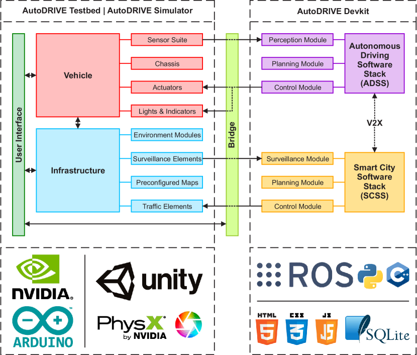
This work does not propose “yet another” research and education platform targeting selective aspects of autonomous driving technology. AutoDRIVE111https://autodrive-ecosystem.github.io (refer Fig. 1) aims to provide a cyber-physical ecosystem that is:
-
•
Comprehensive: The ecosystem offers a scaled car-like vehicle with abundant sensors, which supports single as well as multi-agent algorithms with or without vehicle-to-vehicle (V2V) communication. It also provides a modular infrastructure development kit comprising various environment modules, traffic elements and surveillance elements, which supports internet-of-things (IoT) and vehicle-to-infrastructure (V2I) communication. On the software front, the ecosystem hosts a high-fidelity simulator and supports development of autonomous driving as well as smart city solutions.
-
•
Flexible: The ecosystem offers modular hardware components, a convenient high-fidelity simulator, and an extensive software development support, which enables the end-users to flexibly prototype and validate their autonomy solutions right out-of-the-box. Additionally, the completely open-hardware, open-software architecture of the ecosystem allows users to adapt any of the existing hardware (including design of the vehicle as well as the infrastructure modules) and/or software (including codebase of the development framework as well as the simulator) to better fit their use-cases.
-
•
Integrated: The ecosystem hosts a tightly-coupled trio, comprising AutoDRIVE Devkit (to flexibly develop connected autonomy solutions), AutoDRIVE Simulator (to virtually prototype and test them under a variety of conditions and edge-cases), and AutoDRIVE Testbed (to deploy and validate them in controlled real-world settings). The harmony among these three platforms not only enhances the hardware-software co-development of autonomy solutions, but also helps seamlessly bridge the gap between software simulation and hardware deployment for verification and validation of these safety-critical systems.
This work also describes sample use-cases of four emergent applications in the field of CAVs, with each exploiting, and thus exhibiting, distinct features and capabilities of the AutoDRIVE Ecosystem. These include state-of-the-art (SOTA) implementations such as autonomous parking, behavioral cloning and intersection traversal along with a novel implementation of smart city management.
II State of the Art

Deployment of full-scale CAV solutions generally requires extensive verification and validation, which poses several challenges, especially in university settings. The time, expense, resources and knowledge of full-scale testing interplay with infrastructural requirements as well as safety of personnel and property involved, often hindering research and education progress. Consequently, the past decade has witnessed many university-based deployments exploring development of scaled autonomous vehicles. As described in Table I, such vehicles include the MIT Racecar [5], AutoRally [6], F1TENTH [7], Multi-agent System for non-Holonomic Racing (MuSHR) [8], Optimal RC Racing (ORCA) Project [11], Delft Scaled Vehicle (DSV) [12], and Berkeley Autonomous Race Car (BARC) [13], to name a few. Some of the other community-driven platforms for autonomous driving include HyphaROS RaceCar [9] and Donkey Car [10], both of which are application specific - the former for map-based navigation, and the later for vision-aided imitation learning. Apart from these, commercial products such as QCar [14] by Quanser and DeepRacer [15] by Amazon Web Services (AWS) are now surfacing the market. However, the fact that most of these products are expensive and employ some form of proprietary hardware and/or software components restricts their openness and flexibility to the community; not to mention potential issues like warranty-voids and vendor lock-ins. Some of the other scaled platforms for autonomy research and education include Duckietown [16], TurtleBot3 [17] and Pheeno [18]. However, the differentially-driven robots proposed by these platforms/ecosystems fail to fully satisfy the community requirements for a kinodynamically constrained car-like vehicle.
In terms of comprehensiveness, some of these platforms lack diverse sensing modalities, some lack adequate computational power, some lack Ackermann steering mechanism, and most lack active or passive infrastructural elements. Only a few satisfy the prominent community requirements, but can prove to be prohibitively expensive for university programs.
In terms of flexibility, most of these platforms, if not all, use commercial-off-the-shelf (COTS) radio-controlled (RC) cars as their base-chassis, which: (a) are quite expensive; (b) may not be available all around the world; (c) limit research on the “mechatronics engineering” front, which is equally important for cyber-physical systems such as CAVs. Additionally, most of these platforms only support a specific software framework such as Robot Operating System (ROS) [19], which inherently creates a skillset-dependency for the end-users. Furthermore, providing assets and plugins for pre-packaged simulators like Gazebo [20] or OpenAI Gym [21] environments offers only so much flexibility to the users in terms of designing and running the simulated scenarios.
In terms of integrity, some of these platforms do not support simulation in any form, some ROS-based ones support kinematic/dynamic simulation using RViz [22] and/or Gazebo, while others offer task-specific Gym environments for imitation/reinforcement learning; none of which is ideal.
III AutoDRIVE Testbed

AutoDRIVE Testbed is a hardware platform featuring a native scaled vehicle along with a modular and reconfigurable infrastructure development kit for deploying and validating autonomy algorithms in controlled real-world settings. It adopts a completely open-hardware and open-software architecture so as to push the “systems engineering and integration” front with regard to CAVs.
III-A Vehicle
AutoDRIVE’s native vehicle, named Nigel (refer Fig. 2-A and Fig. 2-B) offers realistic driving and steering actuation, comprehensive sensor suite, high-performance computational resources, and a standard vehicular lighting system.
III-A1 Chassis
Nigel is a 1:14 scale model vehicle comprising four modular platforms, each housing distinct components of the vehicle. It adopts rear wheel drive, Ackermann steered mechanism (refer Fig. 2-C), thereby resembling an actual car in terms of kinodynamic constraints.
III-A2 Power Electronics
Nigel is powered using an 11.1V 5200mAh lithium-polymer (LiPo) battery, whose health is monitored by a voltage checker. A 10A rated buck converter steps down the voltage to 5V, which is then routed, via a 3A rated master switch, to all the electrical sub-systems including a 20A rated motor driver module.
III-A3 Sensor Suite
Nigel hosts a comprehensive sensor suite comprising throttle and steering sensors (actuator feedbacks), 1920 CPR incremental encoders (wheel rotation/velocity), a 3-axis indoor-positioning system (IPS) using fiducial markers (mm/cm-level accurate small-scale positioning analogous to m-level accurate full-scale GNSS), 9-axis IMU (raw inertial data and calibrated AHRS data using Madgwick/Mahony filter), two 62.2∘ FOV cameras with 3.04 mm focal length (front and/or rear RGB frames) and a 7-10 Hz, 360∘ FOV LIDAR with 12 m range and 1∘ resolution (2D laser scan).
III-A4 Computation, Communication and Software
Nigel adopts Jetson Nano Developer Kit - B01 for most of its high-level computation (autonomy algorithms), communication (V2V and V2I) and software installation (JetPack SDK, ROS Melodic and AutoDRIVE Devkit). Additionally, it also hosts Arduino Nano (running the vehicle firmware) for acquiring and filtering raw sensor data and controlling actuators/lights.
III-A5 Actuators
Nigel is provided with two 6V 160 RPM rated 120:1 DC geared motors to drive its rear wheels, and a 9.4 kgf.cm servo motor to steer its front wheels; the steering actuator is saturated at 30∘ w.r.t. zero-steer value. All the actuators are operated at 5V, which translates to a maximum speed of 130 RPM for driving (0.267 m/s @ vehicle) and 0.19 s/60∘ for steering (0.805 rad/s @ vehicle).
III-A6 Lights and Indicators
Nigel’s lighting system comprises of dual-mode headlights, automated taillights, triple-mode turning indicators and automated reverse indicators.
III-B Infrastructure

AutoDRIVE offers a modular and reconfigurable infrastructure development kit (refer Fig. 3) for rapidly designing and prototyping custom driving scenarios. This kit includes a range of environment modules, traffic elements and surveillance elements, along with several preconfigured maps.
III-B1 Environment Modules
Environment modules include static layouts and objects meant for rapidly designing custom scenarios. Apart from these, experts may also choose to design scaled real-world or imaginary scenarios using third-party tools, and import them into AutoDRIVE Ecosystem.
-
•
Terrain Modules: These define off-road segments of the environment. AutoDRIVE currently supports 5 terrains with tunable physical properties (refer Fig. 3-A).
-
•
Road Kits: These enable reconfigurable construction of drivable segments of the environment. AutoDRIVE currently supports 1, 2, 4 and 6 lane road kits, each having 8 different modules (refer Fig. 3-B).
-
•
Obstruction Modules: These 3D objects define static obstacles within the scene. AutoDRIVE currently supports two such modules (refer Fig. 3-C).
III-B2 Traffic Elements
Traffic elements (refer Fig. 3-D) define traffic laws within a particular driving scenario, thereby governing the traffic flow. AutoDRIVE currently supports modular traffic signs and lights. These modules support IoT and V2I communication technologies, and can be therefore integrated with AutoDRIVE Smart City Manager (SCM).
III-B3 Surveillance Elements
AutoDRIVE features a surveillance element called AutoDRIVE Eye to view the entire scene from a bird’s eye view. The said element is also integrated with AutoDRIVE SCM, and, upon calibration of its intrinsic parameters, is capable of estimating vehicle’s 2D pose within the map by detecting and tracking the AprilTag markers attached to each of them; this functionality is illustrated in Fig. 3-E (notice the roof-mounted camera).
III-B4 Preconfigured Maps
AutoDRIVE currently offers 4 preconfigured maps (refer Fig. 3-F). Parking School is designed specifically for autonomous parking applications, wherein construction boxes define static obstacles and all the available free-space is drivable. Driving School covers driving over straight roads, curved roads and crossing an intersection. Intersection School is designed specifically for intersection traversal applications, wherein lane bounds play an important role. Finally, Tiny Town is meant to be a comprehensive driving scenario, which covers each and every infrastructure element currently available in AutoDRIVE.
IV AutoDRIVE Simulator
AutoDRIVE Simulator [23, 24] acts as the digital twin of AutoDRIVE Testbed. It is primarily targeted towards virtual prototyping of autonomy solutions, either for variability testing, or as a part of recursive simulation-deployment workflow, but can also be used for synthetic data generation.
IV-A Vehicle Dynamics Simulation
The vehicle is jointly modelled (refer Fig. 4-A) as a rigid-body and a collection of sprung masses , such that the total mass of the rigid-body is . The rigid-body center of mass is what links the said representations; where are the sprung mass coordinates.
The suspension force acting on each of the sprung masses is ; where, and are the displacements of sprung and unsprung masses, and and are the damping and spring coefficients of -th suspension, respectively.
The wheels of the vehicle are also modelled as rigid-bodies of mass , acted upon by gravitational and suspension forces: .
The tire forces are computed based on the friction curve for each tire: ; where, and are the longitudinal and lateral slips of -th tire, respectively. Here, the friction curve is approximated by a two-piece cubic spline ; where, is a cubic polynomial function. The first segment of the said spline starts at zero and reaches the extremum point , while the other segment starts at the extremum point and saturates at the asymptote point , as shown in the inset of Fig. 4-A.
Now, the tire slip is itself affected by various factors including tire stiffness , steering angle , wheel speeds , suspension forces , and rigid-body momentum , all of which affect the longitudinal/lateral/both components of the linear velocity of the vehicle. Longitudinal slip of -th tire is computed by comparing the longitudinal components of surface velocity of -th wheel (i.e., longitudinal linear velocity of vehicle) with the angular velocity of -th wheel: . Lateral slip of -th tire is dependent on the direction the tire is pointing in and the direction it is moving in, commonly called the slip angle . It is computed by comparing the longitudinal (a.k.a. forward velocity) and lateral (a.k.a. side-slip velocity) components of vehicle’s linear velocity: .
IV-B Sensor Simulation
The simulated vehicle is provided with the same sensing modalities as its real-world counterpart. Particularly, the throttle () and steering () sensors are simulated through a simple feedback loop.
The incremental encoders are simulated by measuring the rotation of rear wheels (i.e., output shaft of driving actuators): ; where, represents ticks measured by -th encoder, is the base resolution (pulses per revolution) of -th encoder, is the gear-ratio of -th motor, and represents the number of revolutions of output shaft of -th motor.
The IPS and IMU are simulated based on temporally-coherent rigid-body transform updates of the vehicle w.r.t. the world : . The IPS provides 3-DOF positional coordinates of the vehicle, whereas the IMU provides linear accelerations , angular velocities and 3-DOF orientation of the vehicle as Euler angles or quaternion .
The LIDAR is simulated using iterative ray-casting raycast{, , } at 7 Hz update rate; where, is the relative transform of LIDAR {} w.r.t. vehicle {} w.r.t. world {}, is the direction vector of each ray-cast , 0.15 m and 12 m are respectively the minimum and maximum linear ranges of LIDAR, and are respectively the minimum and maximum angular ranges of LIDAR, and is the angular resolution of LIDAR. The laser scan ranges are recorded by checking the ray-cast hits and thresholding the minimum linear range of LIDAR: ranges[i]; where, ray.hit is a Boolean flag that checks if a ray-cast hits any colliders in the scene and hit.dist is the Euclidean distance from source of the ray-cast to the hit-point .
The simulated physical cameras are parameterized by their focal length ( 3.04 mm), sensor size ( {3.68, 2.76} mm), target resolution (default = 720p) as well as distance to near and far clipping planes ( 0.01 m and 1000 m). The viewport rendering pipeline for simulated cameras works in 3 stages. First, the camera view matrix is computed by taking the relative homogeneous transform of the camera w.r.t. the world : ; where, and denote rotational and translational components, respectively. Next, the camera projection matrix is computed by projecting the world coordinates to image space coordinates: ; where, and respectively denote distances to near and far clipping planes of the camera, and , , and respectively denote the left, right, top and bottom offsets of the sensor. The camera parameters are related to the projection matrix terms through the following relations: , , . The perspective projection from the simulated camera’s viewport is given by ; where, represents the image space coordinates and represents the world coordinates. Finally, this camera projection is converted into normalized device coordinates (NDC) by performing perspective divide (i.e., dividing throughout by ), obtaining a viewport projection by scaling and shifting the result and then using the rasterization process of the graphics API (e.g., DirectX for Windows, Metal for macOS and Vulkan for Linux). Additionally, a post-processing step simulates lens and film effects of the camera such as lens distortion, depth of field, exposure, ambient occlusion, contact shadows, bloom, motion blur, film grain, chromatic aberration, etc.
IV-C Actuator Simulation
The vehicle is actuated using two driving actuators and a steering actuator, the response delays and saturation limits of which are matched with their real-world counterparts by tuning their torque profiles and actuation limits, respectively.
The driving actuators drive the rear wheels by applying a torque: ; where, is the moment of inertia, is the angular acceleration, is the mass and is the radius of -th wheel. Additionally, the holding torque of the driving actuators is simulated by applying an idle motor torque equivalent to the braking torque: .
The front wheels are steered using a steering actuator, which produces a torque proportional to the required angular acceleration: . The individual turning angles, and , for left and right wheels, respectively, are calculated based on the commanded steering angle , using the Ackermann steering geometry defined by wheelbase and track width , as follows:
IV-D Infrastructure Simulation
Simulated environments can be set-up in one of the following ways:
-
•
AutoDRIVE IDK: The modular and reconfigurable infrastructure development kit (IDK) can be used to create custom scenarios and maps by setting up the terrain modules, road networks, obstruction modules and traffic elements. These assets are present within the simulator source files. Particularly, preconfigured maps depicted in Fig. 3-F-(i), Fig. 3-F-(iii) and Fig. 3-F-(iv) have been constructed using the AutoDRIVE IDK.
-
•
Plug-In Scenarios: AutoDRIVE Simulator supports third-party tools (e.g., RoadRunner [25]) and modular open-source architecture (MOSA) standards (e.g., OpenSCENARIO [26], OpenDRIVE [27], etc.) that enable extensibility. Additionally, users can import a wide array of plugins, packages and assets in a variety of industry-standard formats (e.g., FBX, OBJ, SKP, 3DS, USD, etc.) for developing or customizing driving scenarios. Furthermore, graphics textures designed for AutoDRIVE Testbed can be first imported into the simulator before large-scale printing and setup in real-world. Particularly, preconfigured map depicted in Fig. 3-F-(ii) has been designed using a third-party graphics editing software, imported in AutoDRIVE Simulator and finally printed and setup using AutoDRIVE Testbed.
-
•
Unity Terrain: Being built atop the Unity game engine, AutoDRIVE Simulator natively supports scenario design and development using Unity Terrain [28]. Users can define the terrain mesh, texture, heightmap, vegetation, skybox, wind, etc. to design on-road/off-road scenarios and perform variability testing.
At every time step, the simulator performs mesh-mesh interference detection and computes the contact forces, frictional forces and momentum transfer, along with linear and angular drag acting on the rigid-bodies (refer Fig. 4-B).
IV-E Simulator Features
| Autonomy Algorithm | Platform Exploited | Development Framework | Autonomy Stack | Science and Technology Demonstrated | Agents Involved | Sensors Employed | Actuators Controlled | ||||||||||
|---|---|---|---|---|---|---|---|---|---|---|---|---|---|---|---|---|---|
| Autonomous Parking | AutoDRIVE Testbed |
|
|
|
Single-Agent System | LIDAR |
|
||||||||||
| Behavioral Cloning |
|
|
|
|
Single-Agent System | Front Camera |
|
||||||||||
| Intersection Traversal | AutoDRIVE Simulator | ML-Agents Toolkit (C#) |
|
|
Multi-Agent System |
|
|
||||||||||
| Smart City Management | AutoDRIVE Simulator |
|
|
|
Single-Agent System | None |
|
AutoDRIVE Simulator is developed atop Unity [29] game engine, which employs PhysX [30] for simulating multi-threaded framerate-independent kinematics and dynamics of all the physical entities, and exploits High Definition Render Pipeline (HDRP) [31] along with Post-Processing Stack [32] for rendering photorealistic graphics.
The simulator features an interactive graphical user interface (GUI) consisting of Menu Panel on left-hand side and Heads-Up Display (HUD) on right-hand side. Fig. 4-C depicts the simulator’s GUI with both the panels enabled. The Menu Panel hosts input fields and buttons to configure and control various features of the simulator (refer Fig. 4-D). This includes controls for the communication bridge, along with a series of buttons for (a) toggling between manual and autonomous driving modes for the ego vehicle; (b) switching between the available scene cameras, each providing a distinct view; (c) altering the graphics quality to match the quality-performance trade-off; (d) toggling the scene light to simulate day and night driving conditions; (e) resetting the scene to initial conditions; and (f) quitting the simulator application. The HUD Panel, on the other hand, displays prominent simulation parameters along with vehicle status and sensory data in real-time. It also hosts a time-synchronized data recording functionality, which can be used to export vehicle as well as infrastructure data for a specific run, thereby fostering data-driven approaches aimed at autonomous driving and smart city management.
The simulator natively supports C# scripting, which can be leveraged to customize existing and/or introduce new features, functionalities, modules, behaviors, physics, graphics, communication bridges, APIs and even setup co-simulation frameworks with other simulation tools.
Finally, it is worth mentioning that the simulator, in its source form, has been integrated with various plugins and packages such as the Unity ML Agents Toolkit [33], a machine learning framework for developing and deploying deep imitation/reinforcement learning-based applications directly from within the simulator.
V AutoDRIVE Devkit
AutoDRIVE Devkit is a collection of software packages, application programming interfaces (APIs) and tools, which enables flexible development of autonomous driving as well as smart city management algorithms targeted towards the testbed and/or simulator. It supports both local as well as distributed computing, thereby allowing development of both centralized and decentralized autonomy algorithms.
V-A Autonomous Driving Software Stack
The autonomous driving software stack (ADSS) aids in development of autonomy algorithms specifically targeting the vehicle. It can be used to develop single as well as multi-agent autonomous driving algorithms.
V-A1 ROS Package
AutoDRIVE ROS package supports flexible development of modular autonomy algorithms. It can be installed on a ROS-compatible workstation for interfacing with the simulator (locally/remotely), or directly on Nigel’s on-board computer for hardware deployment.
V-A2 Scripting APIs
AutoDRIVE Devkit currently offers scripting APIs for Python and C++, which can be exploited to develop high-performance autonomy algorithms, without ROS as an intermediary. Such source codes can be interfaced with the simulator (locally/remotely), or directly deployed on Nigel’s on-board computer for hardware validation.
V-B Smart City Software Stack
The smart city software stack (SCSS) aids in development of autonomy algorithms specifically targeting the infrastructure. It can work in tandem with ADSS to develop smart city applications pertaining to traffic management.
V-B1 SCM Server
AutoDRIVE Devkit offers a centralized Smart City Manager (SCM) server to monitor and control various “smart” elements. The server hosts a database to keep track of all the vehicles along with active and passive traffic elements within a particular scene.
V-B2 SCM Webapp
AutoDRIVE SCM hosts an interactive webapp, which allows the users to connect with the database for monitoring and controlling the traffic flow in real-time.
VI Demonstration Case-Studies


This work showcases key features and capabilities of the AutoDRIVE Ecosystem through 4 carefully shortlisted case-studies (refer Table II). Although this paper cannot furnish exhaustive details pertaining to any particular demonstration, we recommend interested readers to peruse this technical report [34].
It is to be noted that the presented demonstrations are by no means exhaustive and that AutoDRIVE Ecosystem can be employed to develop, simulate and deploy a much wider array of applications including (but not limited to) synthetic/real/hybrid data collection and labeling; traditional (e.g., deterministic/probabilistic, classical/optimal, etc.) as well as modern (e.g., deep imitation/reinforcement/hybrid learning, etc.) algorithms for perception, state estimation, path/motion planning and motion control; modular as well as end-to-end autonomy stacks; benchmarking existing solutions (education) or innovating novel scientific and technological approaches for autonomy (research), etc.
VI-A Autonomous Parking
This demonstration leveraged AutoDRIVE’s ROS-enabled capabilities to demonstrate autonomous parking (refer Fig. 5-A). First, the vehicle mapped its surroundings using Hector SLAM algorithm [35] (refer Fig. 5-B). It could then localize itself against this known static map using range-flow-based odometry [36] (refer Fig. 5-C) and adaptive particle filter algorithm [37] (refer Fig. 5-D). For autonomous navigation, the vehicle planned a feasible global path from its current pose to parking pose using A* algorithm [38], while also re-planning its local trajectory for dynamic collision avoidance using timed-elastic-band approach [39]. A proportional controller generated driving (throttle/brake) and steering commands for the vehicle to track the local trajectory (refer Fig. 5-E). Future work in this direction can include benchmarking of various SOTA and/or novel algorithms for mapping, localization, path planning and motion control.


VI-B Behavioral Cloning
This demonstration was based on [40], wherein the objective was to employ a convolutional neural network (CNN) [41] for cloning the end-to-end driving behavior of a human. As such, AutoDRIVE Simulator was exploited to record 5-laps worth of temporally-coherent labeled manual driving data, which was balanced, augmented and pre-processed using standard computer vision techniques, to train a 6-layer deep CNN (refer Fig. 6-A). Post training for 4 epochs, with a learning rate of 1e-3 using the Adam optimizer [42], the training and validation losses converged stably without over/under-fitting. The trained model was then deployed back into the virtual world to validate its performance through activation and prediction analyses (refer Fig. 6-B). Further, the same model was transferred to AutoDRIVE Testbed for validating sim2real capability of the ecosystem through activation and prediction analyses (refer Fig. 6-C). In order to have a zero-shot sim2real transition: (i) the physical and visual aspects of virtual world were setup as close to the real world as possible, and (ii) the exhaustive data augmentation pipeline implicitly performed domain randomization. However, further investigation is required to comment on and improve the robustness of sim2real transfer considering sensor simulation, vehicle modeling and scenario representation. Finally, although this work adopted a coupled-control law for vehicle motion smoothing, a potential improvement could be to investigate independent actuation smoothing techniques like low-pass filters or proximal bounds.
VI-C Intersection Traversal
Inspired from [43], this work demonstrates single and multi-agent (refer Fig. 7-A) intersection traversal using deep reinforcement learning (refer Fig. 7-B). Each agent collected a vectorized observation , including its relative goal location , along with relative location , relative yaw and velocity of its peers obtained through V2V communication. The action space of each agent, , included discretized steering and constant throttle (). An extrinsic reward function kept agents in check while training a 3-layer fully-connected neural network based policy, , using PPO algorithm [44] (refer Fig. 7-C). This ultimately resulted in all agents being able to traverse the intersection safely (refer Fig. 7-D). Although we could not implement this application in real-world owing to monetary constraints, investigating the sim2real transition of this application would be a natural progression of this work. Additionally, application of actuation smoothing techniques could be a potential improvement.
VI-D Smart City Management
This novel use case of smart city traffic management was possible due to AutoDRIVE’s V2I and IoT capabilities. As depicted in Fig. 8-A), the SCM server hosted a database to keep track of all the traffic elements, and acted as a high-level behavior planner for the ego vehicle. It switched the vehicle behavior upon detecting respective traffic signs and lights by setting the appropriate throttle and steering trims, which were then passed on to proximally optimal predictive (POP) controller coupled with adaptive longitudinal controller (ALC) [45]. Finally, SCM server teleoperated the vehicle to achieve the mission objective (refer Fig. 8-B). A natural progression of this work would be to implement a multi-agent scenario, preferably within a mixed-reality digital-twin setting, to investigate different strategies for efficient smart city traffic management.
VII Summary
AutoDRIVE was developed with an aim of tightly integrating real and virtual worlds into a common toolchain, without compromising on the comprehensiveness, flexibility and accessibility required for prototyping and validating autonomy solutions. It has numerous applications, which are bound to increase as the ecosystem is upgraded. Potential improvements include supporting heterogeneous vehicles and robotic pedestrians, full-scale vehicles and environments, expanding API support and adding extended reality capabilities, to name a few. We hope that the community benefits from adopting this ecosystem, may it be for education, research or anything in between.
VIII Supplemental Material
AutoDRIVE Ecosystem is openly accessible.
-
•
AutoDRIVE Ecosystem Website:
https://AutoDRIVE-Ecosystem.github.io -
•
AutoDRIVE Ecosystem GitHub Organization:
https://github.com/AutoDRIVE-Ecosystem -
•
AutoDRIVE Ecosystem YouTube Channel:
https://www.youtube.com/@AutoDRIVE-Ecosystem
References
- [1] E. Yurtsever, J. Lambert, A. Carballo, and K. Takeda, “A Survey of Autonomous Driving: Common Practices and Emerging Technologies,” IEEE Access, vol. 8, pp. 58 443–58 469, 2020.
- [2] A. Dosovitskiy, G. Ros, F. Codevilla, A. Lopez, and V. Koltun, “CARLA: An Open Urban Driving Simulator,” in Proceedings of the 1st Annual Conference on Robot Learning, ser. Proceedings of Machine Learning Research, S. Levine, V. Vanhoucke, and K. Goldberg, Eds., vol. 78. PMLR, 13-15 Nov 2017, pp. 1–16. [Online]. Available: http://proceedings.mlr.press/v78/dosovitskiy17a.html
- [3] G. Rong, B. H. Shin, H. Tabatabaee, Q. Lu, S. Lemke, M. Možeiko, E. Boise, G. Uhm, M. Gerow, S. Mehta, E. Agafonov, T. H. Kim, E. Sterner, K. Ushiroda, M. Reyes, D. Zelenkovsky, and S. Kim, “LGSVL Simulator: A High Fidelity Simulator for Autonomous Driving,” in 2020 IEEE 23rd International Conference on Intelligent Transportation Systems (ITSC), 2020, pp. 1–6.
- [4] S. Shah, D. Dey, C. Lovett, and A. Kapoor, “AirSim: High-Fidelity Visual and Physical Simulation for Autonomous Vehicles,” in Field and Service Robotics, M. Hutter and R. Siegwart, Eds. Cham: Springer International Publishing, 2018, pp. 621–635.
- [5] S. Karaman, A. Anders, M. Boulet, J. Connor, K. Gregson, W. Guerra, O. Guldner, M. Mohamoud, B. Plancher, R. Shin, and J. Vivilecchia, “Project-based, collaborative, algorithmic robotics for high school students: Programming self-driving race cars at MIT,” in 2017 IEEE Integrated STEM Education Conference (ISEC), 2017, pp. 195–203. [Online]. Available: https://mit-racecar.github.io
- [6] B. Goldfain, P. Drews, C. You, M. Barulic, O. Velev, P. Tsiotras, and J. M. Rehg, “AutoRally: An Open Platform for Aggressive Autonomous Driving,” IEEE Control Systems Magazine, vol. 39, no. 1, pp. 26–55, 2019. [Online]. Available: https://arxiv.org/abs/1806.00678
- [7] M. O’Kelly, V. Sukhil, H. Abbas, J. Harkins, C. Kao, Y. V. Pant, R. Mangharam, D. Agarwal, M. Behl, P. Burgio, and M. Bertogna. (2019) F1/10: An Open-Source Autonomous Cyber-Physical Platform. [Online]. Available: https://arxiv.org/abs/1901.08567
- [8] S. S. Srinivasa, P. Lancaster, J. Michalove, M. Schmittle, C. Summers, M. Rockett, J. R. Smith, S. Choudhury, C. Mavrogiannis, and F. Sadeghi. (2019) MuSHR: A Low-Cost, Open-Source Robotic Racecar for Education and Research. [Online]. Available: https://arxiv.org/abs/1908.08031
- [9] HyphaROS Workshop, “HyphaROS Racecar,” 2021. [Online]. Available: https://github.com/Hypha-ROS/hypharos_racecar
- [10] Donkey Community, “An Open-Source DIY Self-Driving Platform for Small-Scale Cars,” 2021. [Online]. Available: https://www.donkeycar.com
- [11] Automatic Control Laboratory, ETH Zürich, “ORCA (Optimal RC Racing) Project,” 2021. [Online]. Available: https://control.ee.ethz.ch/research/team-projects/autonomous-rc-car-racing.html
- [12] T. Kalidien, P. van der Burg, A. Mulder, E. Rietveld, M. Vonk, H. Hellendoorn, and M. Alirezaei, “Design and Development of the Delft Scaled Vehicle: A Platform for Autonomous Driving Tests,” Delft Center for Systems & Control, Delft University of Technology, Delft, Netherlands, Bachelor’s Thesis, 2017. [Online]. Available: https://www.erwinrietveld.com/assets/docs/BEP11_DSCS_Paper_Final.pdf
- [13] J. Pappas, C. H. Yuan, C. S. Lu, N. Nassar, A. Miller, S. van Leeuwen, and F. Borrelli, “Berkeley Autonomous Race Car (BARC),” 2021. [Online]. Available: https://sites.google.com/site/berkeleybarcproject
- [14] Quanser Consulting Inc., “QCar - A Sensor-Rich Autonomous Vehicle,” 2021. [Online]. Available: https://www.quanser.com/products/qcar
- [15] Amazon Web Services, “AWS DeepRacer,” 2021. [Online]. Available: https://aws.amazon.com/deepracer
- [16] L. Paull, J. Tani, H. Ahn, J. Alonso-Mora, L. Carlone, M. Cap, Y. F. Chen, C. Choi, J. Dusek, Y. Fang, D. Hoehener, S.-Y. Liu, M. Novitzky, I. F. Okuyama, J. Pazis, G. Rosman, V. Varricchio, H.-C. Wang, D. Yershov, H. Zhao, M. Benjamin, C. Carr, M. Zuber, S. Karaman, E. Frazzoli, D. Del Vecchio, D. Rus, J. How, J. Leonard, and A. Censi, “Duckietown: An Open, Inexpensive and Flexible Platform for Autonomy Education and Research,” in 2017 IEEE International Conference on Robotics and Automation (ICRA), 2017, pp. 1497–1504. [Online]. Available: http://michalcap.net/wp-content/papercite-data/pdf/paull_2017.pdf
- [17] Robotis Inc., “TurtleBot3,” 2021. [Online]. Available: https://emanual.robotis.com/docs/en/platform/turtlebot3/overview/
- [18] S. Wilson, R. Gameros, M. Sheely, M. Lin, K. Dover, R. Gevorkyan, M. Haberland, A. Bertozzi, and S. Berman, “Pheeno, A Versatile Swarm Robotic Research and Education Platform,” IEEE Robotics and Automation Letters, vol. 1, no. 2, pp. 884–891, 2016.
- [19] M. Quigley, K. Conley, B. Gerkey, J. Faust, T. Foote, J. Leibs, R. Wheeler, and A. Ng, “ROS: an open-source Robot Operating System,” in ICRA 2009 Workshop on Open Source Software, vol. 3, Jan 2009. [Online]. Available: http://robotics.stanford.edu/~ang/papers/icraoss09-ROS.pdf
- [20] N. P. Koenig and A. Howard, “Design and use paradigms for Gazebo, an open-source multi-robot simulator,” in 2004 IEEE/RSJ International Conference on Intelligent Robots and Systems (IROS) (IEEE Cat. No.04CH37566), vol. 3, 2004, pp. 2149–2154.
- [21] G. Brockman, V. Cheung, L. Pettersson, J. Schneider, J. Schulman, J. Tang, and W. Zaremba. (2016) OpenAI Gym. [Online]. Available: https://arxiv.org/abs/1606.01540
- [22] D. Hershberger, D. Gossow, and J. Faust, “RViz: 3D Visualization Tool for ROS,” 2021. [Online]. Available: http://wiki.ros.org/rviz
- [23] T. V. Samak, C. V. Samak, and M. Xie, “AutoDRIVE Simulator: A Simulator for Scaled Autonomous Vehicle Research and Education,” in 2021 2nd International Conference on Control, Robotics and Intelligent System, ser. CCRIS’21. New York, NY, USA: Association for Computing Machinery, 2021, p. 1–5. [Online]. Available: https://doi.org/10.1145/3483845.3483846
- [24] T. V. Samak and C. V. Samak, “AutoDRIVE Simulator - Technical Report,” 2022. [Online]. Available: https://arxiv.org/abs/2211.07022
- [25] Mathworks Inc., “RoadRunner,” 2021. [Online]. Available: https://www.mathworks.com/products/roadrunner.html
- [26] Association for Standardization of Automation and Measuring Systems (ASAM), “OpenSCENARIO,” 2021. [Online]. Available: https://www.asam.net/standards/detail/openscenario
- [27] ——, “OpenDRIVE,” 2021. [Online]. Available: https://www.asam.net/standards/detail/opendrive
- [28] Unity Technologies, “Unity Terrain,” 2021. [Online]. Available: https://docs.unity3d.com/Manual/script-Terrain.html
- [29] ——, “Unity,” 2021. [Online]. Available: https://unity.com
- [30] NVIDIA GameWorks, “NVIDIA PhysX SDK 4.1,” 2021. [Online]. Available: https://github.com/NVIDIAGameWorks/PhysX-3.4
- [31] Unity Technologies Technical Marketing, “Unity Scriptable Render Pipeline,” 2021. [Online]. Available: https://github.com/UnityTechnologies/ScriptableRenderPipeline
- [32] Unity Technologies, “Post-Processing Stack v2,” 2021. [Online]. Available: https://github.com/Unity-Technologies/PostProcessing
- [33] A. Juliani, V.-P. Berges, E. Teng, A. Cohen, J. Harper, C. Elion, C. Goy, Y. Gao, H. Henry, M. Mattar, and D. Lange, “Unity: A General Platform for Intelligent Agents,” 2018. [Online]. Available: https://arxiv.org/abs/1809.02627
- [34] T. V. Samak and C. V. Samak, “AutoDRIVE - Technical Report,” 2022. [Online]. Available: https://arxiv.org/abs/2211.08475
- [35] S. Kohlbrecher, O. von Stryk, J. Meyer, and U. Klingauf, “A Flexible and Scalable SLAM System with Full 3D Motion Estimation,” in 2011 IEEE International Symposium on Safety, Security, and Rescue Robotics, 2011, pp. 155–160. [Online]. Available: http://doi.org/10.1109/SSRR.2011.6106777
- [36] M. Jaimez, J. G. Monroy, and J. Gonzalez-Jimenez, “Planar Odometry from a Radial Laser Scanner. A Range Flow-based Approach,” in 2016 IEEE International Conference on Robotics and Automation (ICRA), 2016, pp. 4479–4485. [Online]. Available: http://doi.org/10.1109/ICRA.2016.7487647
- [37] D. Fox, “KLD-Sampling: Adaptive Particle Filters,” in Advances in Neural Information Processing Systems, T. Dietterich, S. Becker, and Z. Ghahramani, Eds., vol. 14. MIT Press, 2001. [Online]. Available: https://proceedings.neurips.cc/paper/2001/file/c5b2cebf15b205503560c4e8e6d1ea78-Paper.pdf
- [38] P. E. Hart, N. J. Nilsson, and B. Raphael, “A Formal Basis for the Heuristic Determination of Minimum Cost Paths,” IEEE Transactions on Systems Science and Cybernetics, vol. 4, no. 2, pp. 100–107, 1968. [Online]. Available: http://doi.org/10.1109/TSSC.1968.300136
- [39] C. Rösmann, F. Hoffmann, and T. Bertram, “Kinodynamic Trajectory Optimization and Control for Car-Like Robots,” in 2017 IEEE/RSJ International Conference on Intelligent Robots and Systems (IROS), 2017, pp. 5681–5686. [Online]. Available: http://doi.org/10.1109/IROS.2017.8206458
- [40] T. V. Samak, C. V. Samak, and S. Kandhasamy, “Robust behavioral cloning for autonomous vehicles using end-to-end imitation learning,” SAE International Journal of Connected and Automated Vehicles, vol. 4, no. 3, pp. 279–295, aug 2021. [Online]. Available: https://doi.org/10.4271/12-04-03-0023
- [41] A. Krizhevsky, I. Sutskever, and G. E. Hinton, “ImageNet Classification with Deep Convolutional Neural Networks,” in Advances in Neural Information Processing Systems, F. Pereira, C. Burges, L. Bottou, and K. Weinberger, Eds., vol. 25. Curran Associates, Inc., 2012. [Online]. Available: https://proceedings.neurips.cc/paper/2012/file/c399862d3b9d6b76c8436e924a68c45b-Paper.pdf
- [42] D. P. Kingma and J. Ba, “Adam: A Method for Stochastic Optimization,” 2014. [Online]. Available: https://arxiv.org/abs/1412.6980
- [43] K. Sivanathan, B. K. Vinayagam, T. Samak, and C. Samak, “Decentralized motion planning for multi-robot navigation using deep reinforcement learning,” in 2020 3rd International Conference on Intelligent Sustainable Systems (ICISS), 2020, pp. 709–716.
- [44] J. Schulman, F. Wolski, P. Dhariwal, A. Radford, and O. Klimov, “Proximal policy optimization algorithms,” 2017. [Online]. Available: https://arxiv.org/abs/1707.06347
- [45] C. V. Samak, T. V. Samak, and S. Kandhasamy, “Proximally optimal predictive control algorithm for path tracking of self-driving cars,” in Advances in Robotics - 5th International Conference of The Robotics Society, ser. AIR2021. New York, NY, USA: Association for Computing Machinery, 2022. [Online]. Available: https://doi.org/10.1145/3478586.3478632