Augmented physics informed extreme learning machine to solve the biharmonic equations via Fourier expansions

This section provides a detailed introduction to the PIELM method for solving the biharmonic equation (1) with boundaries (2) or (3). To obtain an ideal solution to the biharmonic equation, one can seek the solution in trial function space spanned by the ELM model with a high-order smooth activation function. Then, an ansatz expressed by ELM is designed to approximate the solutions of (1), it is:

Substituting $u(\bm{x};\bm{W},\bm{b})$ into the equation of (1) for $u$, we can obtain the following equation

with $V_{i}(\bm{x})=\bm{x}^{T}\cdot\bm{W}^{[i]}+b_{i}$ being the linear output for $i_{th}$ hidden unit of ELM and $N$ is the number of hidden unit. Additionally, $u(\bm{x};\bm{W},\bm{b})$ still holds on the prescribed boundaries (2) or (3), we then have the following formulation

or

For solving the biharmonic equations by the aforementioned PIELM method, a collection of collocation points is sampled from both the interior and boundaries of the domain. At these collocation points, the governed function (5) and the (6) or (7) exhibit coerciveness. Let $Q$ denote the number of random collocation points in the interior of $\Omega$ and denote by $\mathcal{S}_{I}=\{\bm{x}_{I}^{q}\}_{q=1}^{Q}$, and $P$ denote the number of random collocation points on hyperface of $\partial\Omega$ and denote by $\mathcal{S}_{B}=\{\bm{x}_{B}^{p}\}_{p=1}^{P}$. Feeding the above collocation points into the pipeline of PIELM, we have the following residual terms for Dirichlet boundaries:

and the last term in (8) will be replaced by

for Navier boundaries.

To approximate the functions $u$ well, we need to adjust the output weights of the PIELM model to make each residual of (8) to near-zero or minimize the error of the following system of linear equations:

Here $\displaystyle\mathbf{H}_{f}=\mathbf{H}_{B}+\sum_{i=1}^{d}\sum_{j=1,j\neq i}^{d}\mathbf{H}_{ij}$ with

and

Additionally, the matrices $\mathbf{H}_{g}$, $\mathbf{H}_{h}$ and $\mathbf{H}_{k}$ are given by

$\displaystyle\mathbf{H}_{h}=\mathbf{H}_{1}\cdot n_{1}+\mathbf{H}_{2}\cdot n_{2}+\cdots+\mathbf{H}_{d}\cdot n_{d}$ with

and

In the above expressions, $\sigma^{\prime\prime}$ and $\sigma^{\prime\prime\prime\prime}$ are the second and fourth-order derivatives of activation function $\sigma$, respectively, and $\bigodot$ stands for the Hadamard product operator. In addition, $\mathbf{S}_{f}=\big{(}f(\bm{x}_{I}^{1}),f(\bm{x}_{I}^{2}),\cdots,f(\bm{x}_{I}^{Q})\big{)}^{T}$, $\mathbf{S}_{g}=\big{(}g(\bm{x}_{B}^{1}),g(\bm{x}_{B}^{2}),\cdots,g(\bm{x}_{B}^{P})\big{)}^{T}$, $\mathbf{S}_{h}=\big{(}h(\bm{x}_{B}^{1}),h(\bm{x}_{B}^{2}),\cdots,h(\bm{x}_{B}^{P})\big{)}^{T}$ and $\mathbf{S}_{k}=\big{(}k(\bm{x}_{B}^{1}),k(\bm{x}_{B}^{2}),\cdots,k(\bm{x}_{B}^{P})\big{)}^{T}$.

When the weights and biases of the hidden layer for the PIELM model are randomly initialized and fixed, the matrix $\mathbf{H}$ is determined for given input data, then the output weights $\bm{\beta}$ of PIELM model are obtained by solving the linear systems (10). The system equation $\mathbf{H}\bm{\beta}=\mathbf{S}$ is solvable and meets the following several cases:

• 1.

  If the coefficient matrix $\mathbf{H}$ is square and invertible, then

  $$\bm{\beta}=\mathbf{H}^{-1}\mathbf{S}.$$

  (11)

• 2.

  If the coefficient matrix $\mathbf{H}$ is rectangular and full rank, then

  $$\bm{\beta}=\mathbf{H}^{\dagger}\mathbf{S},$$

  (12)

  where $\mathbf{H}^{\dagger}$ is the pseudo inverse of $\mathbf{H}$ defned by $\mathbf{H}^{\dagger}=(\mathbf{H}^{T}\mathbf{H})^{-1}\mathbf{H}^{T}$.

• 3.

  If the coefficient matrix $\mathbf{H}$ is singular, then the Tikhonov regularization[51] can be utilized to to overcome the ill-posedness of (10), and the $\bm{\beta}$ is given by

  $$\bm{\beta}=(\mathbf{H}^{T}\mathbf{H}+\lambda\mathbf{I})^{-1}\mathbf{H}\mathbf{S},$$

  (13)

  where $\mathbf{I}$ is the identity matrix, and $\lambda>0$ is the ridge parameter.

According to the above discussions, the detailed procedures involved in the PIELM algorithm to address the biharmonic equation (1) within finite-dimensional spaces are described in the following.

In terms of function approximation, the hidden nodes governed by a given activation function in the ELM model can be considered a set of basis functions, and then the ELM model produces its output through a linear aggregation of these fundamental functions. Similar to other artificial neural network (ANN) architectures, the choice of activation function is critical for the ELM model’s performance. Since the biharmonic equations (1) studied here is a high-order PDE, activation functions with strong regularity are preferred. Previous studies, including Fabiani et al. [40], Calabrò et al. [41], and Ma et al. [52], have investigated the influence of sigmoidal functions and radial basis functions in the ELM model for solving both linear and nonlinear PDEs. These studies indicate that ELM models with sigmoid, Gaussian, and tangent activation functions achieve commendable numerical accuracy.

The sigmoid, gaussian, and tangent functions all fulfill the Lipschitz continuity and exhibit robust regularity, they ensure the boundedness of the output for hidden units in ELM. In terms of the high-order PDEs, the high-order derivate of activation is required. Then, the first, second, and fourth-order derivatives for the sigmoidal function $s(x)=1/(1+e^{-x})$, Gaussian function $\sigma(x)=e^{-x^{2}}$ and hyperbolic tangent function $tanh(x)=(e^{x}-e^{-x})/(e^{x}+e^{-x})$ are given by

and

respectively. Figs. 2 – 4 illustrate the curves of the sigmoid, Gaussian, and tangent functions and their corresponding first-order, second-order and fourth-order derivatives, respectively.

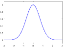
This visualization shows that the derivatives of the sigmoid, Gaussian, and tanh functions are bounded and tend to saturate for narrow-range inputs. However, their performance may degrade with large-range inputs. Inspired by the Fourier-based spectral method, a global basis function can generate responses, along with its derivatives, for both narrow- and large-range inputs. Furthermore, approximations based on such basis functions can handle data across various scales. The sine function serves as an ideal global Fourier basis function (with sine and cosine being fundamentally equivalent). In this study, we adopt the sine function as the activation function in the PIELM method, referring to this modified approach as FPIELM.

In this section, we apply the proposed FPIELM method to solve the two- and three-dimensional biharmonic equation (1) in both unitized and non-unitized domains. Additionally, PIELM models using Sigmoid, Gaussian, and Tanh as activation functions are established as baselines for solving (1) and are referred to as SPIELM, GPIELM, and TPIELM, respectively. Following the results in Dong and Yang [46], the weight matrices and bias vectors for the hidden layers of each model are initialized uniformly within the interval $[-\delta,\delta]$.

A criterion is provided to evaluate the performance of the four aforementioned methods, given by

where $\tilde{u}(\bm{x}^{i})$ and $u^{*}(\bm{x}^{i})$ denote the approximate solution obtained by numerical methods and the exact solution, respectively, for the collection set $\{\bm{x}^{i}\}_{i=1}^{N^{\prime}}$, with $N^{\prime}$ being the number of collection points.

All experiments are implemented in Numpy (version 1.21.0) on a workstation equipped with 256 GB RAM and a single NVIDIA GeForce RTX 4090 Ti GPU with 24 GB of memory.

First, we approximate the solution of (1) using the four methods on 16,384 equidistant grid points distributed across regular domains: $[-1,1]\times[-1,1]$, $[0,5]\times[0,5]$, $[-4,6]\times[-3,7]$, and $[5,15]\times[0,10]$. In addition to the grid points, the training set includes 10,000 random points within $\Omega$ and 4,000 random points on $\partial\Omega$. The number of hidden nodes for each of the four PIELM methods is set to 1,000.

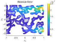
Figure 5 shows the point-wise absolute error of the four PIELM models on the domain $[-1,1]\times[-1,1]$. Table 1 presents the optimal value of $\delta$, the REL, and the runtime for each PIELM method across the different domains.

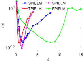
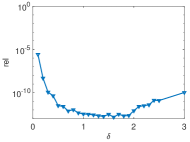
Next, we examine the impact of the scale factor $\delta$ and the number of hidden nodes on the FPIELM model in the domain $[-1,1]\times[-1,1]$, with results illustrated in Fig. 6. Finally, comparison curves for REL as a function of the scale factor $\delta$ for the four PIELM methods on the domains $[-1,1]\times[-1,1]$ and $[0,5]\times[0,5]$ are shown in Fig. 7.

Based on the point-wise absolute error distribution shown in Figures 5(b) – 5(e) and the data in Table 1, it can be concluded that the FPIELM method outperforms other types of PIELM methods. As observed in the curves in Figure 6(a), the relative error does not decrease with an increasing number of hidden units, indicating that the performance of the FPIELM model stabilizes as the number of hidden neurons grows. The time-neuron curve in Figure 6(b) demonstrates a superlinear increase in runtime with the addition of hidden neurons, though this increase is gradual. Furthermore, Figure 6(c) illustrates that the FPIELM model remains stable and robust across variations in the scale factor $\sigma$ on the domain $[-1,1]\times[-1,1]$. The REL curves in Figure 7 confirm that FPIELM maintains stability and allows for a broader range of scale factor $\delta$ values across both unitized and non-unitized domains. In summary, our FPIELM method not only achieves high accuracy but also demonstrates efficiency and robustness. Additionally, it is noteworthy that the coefficient matrix in the final linear system is full rank, given that the number of samples exceeds the number of hidden nodes.

For comparison, we employ the finite difference method (FDM) with a five-point central difference scheme to solve the coupled scheme of (1) on the domain $[0,5]\times[0,5]$. The FDM is implemented in MATLAB (version 12.0.0.341360, R2019a). For the FPIELM model, the number of hidden nodes is set to 1,000, and the scale factor $\delta$ for initializing weights and biases is set to 5.0. The numerical results in Table 2 indicate that the proposed FPIELM method maintains stability across various mesh grid sizes and significantly outperforms FDM in terms of accuracy, particularly on sparse grids.

In this example, the setup for the four PIELM methods is identical to that in Example 4.1. An approximate solution to (1) is derived by applying the four methods on 19,214 collection points located within the hexagram domains $\Omega$. Numerical results are presented in Table 3 for the two scenarios, and the point-wise absolute error for the four PIELM methods is shown in Figure 8 over the hexagram domain derived from $[-\pi,\pi]\times[-\pi,\pi]$.

Additionally, Figure 9 illustrates the variation in relative error and runtime concerning the number of hidden nodes, as well as the variation in relative error with the scale factor $\delta$ for FPIELM on the hexagram domain derived from $[-\pi,\pi]\times[-\pi,\pi]$. Finally, Figure 10 plots the REL comparison curves for the four PIELM methods, showing how REL varies with the scale factor $\delta$ across the hexagram domains derived from $[-\pi,\pi]\times[-\pi,\pi]$ and $[0,3\pi]\times[\pi,2\pi]$.

Based on the data in Table 3 and the point-wise absolute errors depicted in Figs. 8(b) – 8(e), we can infer that the FPIELM method outperforms the PIELM methods with sigmoid, tanh, and Gaussian activation functions. As observed in the curves in Fig. 16(a), the performance of the FPIELM method stabilizes as the number of hidden nodes increases. The time-neuron curve in Fig. 16(b) shows that the runtime exhibits a superlinear increase with the growing number of hidden nodes, although the increase remains gradual. Lastly, Figs. 9(c) and 10 illustrate that the FPIELM method remains stable and robust across variations in the scale factor $\sigma$. In summary, our FPIELM method demonstrates not only high accuracy but also efficiency and robustness.

In this example, the number of hidden units for each of the four PIELM methods is set to 2,000. The testing set consists of 40,000 random points within the cut planes, excluding the holes, and includes planes parallel to the $xoy$ and $yoz$ coordinate planes. Additionally, 6,000 points randomly sampled from the six boundary surfaces are integrated into the testing set. The results are presented in Figs. 12 – 14.

Based on the point-wise error shown in Figs. 12(b) – 12(e), our proposed FPIELM method outperforms the other three methods in solving the biharmonic equation (1) in three-dimensional space. The relative errors presented in Fig. 14 indicate that the FPIELM method remains stable across various scale factors $\delta$ and is superior to the other methods. Furthermore, the curves of relative error and runtime in Fig. 13 demonstrate the favorable stability and robustness of the FPIELM method as both the number of hidden nodes and the scale factor $\delta$ increase. It is also noteworthy that the coefficient matrix in the final linear system is full rank for this example, eliminating the need for adjustment through Tikhonov regularization.

In this example, the setup for the four PIELM methods is identical to that in Example 4.1. An approximate solution of (1) is obtained by applying the four methods on 16,384 grid points within the rectangular domains $[0,1]\times[0,1]$ and $[0,4]\times[0,4]$. The numerical results are listed in Table 4 for these two scenarios, and the point-wise absolute error for the four PIELM methods is shown in Fig. 15 on the domain $[0,1]\times[0,1]$.

Additionally, Fig. 16 illustrates the variation in relative error and runtime concerning the number of hidden nodes, as well as the variation in relative error with the scale factor $\delta$ for FPIELM on the domain $[0,1]\times[0,1]$. Finally, Fig. 17 plots the comparison curves for REL as a function of the scale factor $\delta$ for the four PIELM methods on the rectangular domains $[0,1]\times[0,1]$ and $[0,4]\times[0,4]$, respectively.

References

- Wahba [1990] G. Wahba, Spline models for observational data, SIAM, 1990.
- Greengard and Kropinski [1998] L. Greengard, M. C. Kropinski, An integral equation approach to the incompressible navier–stokes equations in two dimensions, SIAM Journal on Scientific Computing 20 (1998) 318–336.
- Ferziger and PeriC [2002] J. H. Ferziger, M. PeriC, Computational methods for fluid dynamics, Springer, 2002.
- Christiansen [1975] S. Christiansen, Integral equations without a unique solution can be made useful for solving some plane harmonic problems, IMA Journal of Applied Mathematics 16 (1975) 143–159.
- Constanda [1995] C. Constanda, The boundary integral equation method in plane elasticity, Proceedings of the American Mathematical Society 123 (1995) 3385–3396.
- Gupta and Manohar [1979] M. M. Gupta, R. P. Manohar, Direct solution of the biharmonic equation using noncoupled approach, Journal of Computational Physics 33 (1979) 236–248.
- Altas et al. [1998] I. Altas, J. Dym, M. M. Gupta, R. P. Manohar, Multigrid solution of automatically generated high-order discretizations for the biharmonic equation, SIAM Journal on Scientific Computing 19 (1998) 1575–1585.
- Ben-Artzi et al. [2008] M. Ben-Artzi, J.-P. Croisille, D. Fishelov, A fast direct solver for the biharmonic problem in a rectangular grid, SIAM Journal on Scientific Computing 31 (2008) 303–333.
- Bialecki [2012] B. Bialecki, A fourth order finite difference method for the dirichlet biharmonic problem, Numerical Algorithms 61 (2012) 351–375.
- Bi and Li [2004] C.-J. Bi, L.-K. Li, Mortar finite volume method with adini element for biharmonic problem, Journal of Computational Mathematics (2004) 475–488.
- Wang [2004] T. Wang, A mixed finite volume element method based on rectangular mesh for biharmonic equations, Journal of Computational and Applied Mathematics 172 (2004) 117–130.
- Eymard et al. [2012] R. Eymard, T. Gallouët, R. Herbin, A. Linke, Finite volume schemes for the biharmonic problem on general meshes, Mathematics of Computation 81 (2012) 2019–2048.
- Baker [1977] G. A. Baker, Finite element methods for elliptic equations using nonconforming elements, Mathematics of Computation 31 (1977) 45–59.
- Lascaux and Lesaint [1975] P. Lascaux, P. Lesaint, Some nonconforming finite elements for the plate bending problem, Revue française d’automatique, informatique, recherche opérationnelle. Analyse numérique 9 (1975) 9–53.
- Morley [1968] L. S. D. Morley, The triangular equilibrium element in the solution of plate bending problems, Aeronautical Quarterly 19 (1968) 149–169.
- Zienkiewicz et al. [2013] O. C. Zienkiewicz, R. L. Taylor, P. Nithiarasu, The finite element method for fluid dynamics, Butterworth-Heinemann, 2013.
- Ciarlet [2002] P. G. Ciarlet, The finite element method for elliptic problems, SIAM, 2002.
- Brezzi and Fortin [2012] F. Brezzi, M. Fortin, Mixed and hybrid finite element methods, volume 15, Springer Science & Business Media, 2012.
- Cheng et al. [2000] X.-l. Cheng, W. Han, H.-c. Huang, Some mixed finite element methods for biharmonic equation, Journal of computational and applied mathematics 126 (2000) 91–109.
- Davini and Pitacco [2000] C. Davini, I. Pitacco, An unconstrained mixed method for the biharmonic problem, SIAM Journal on Numerical Analysis 38 (2000) 820–836.
- Lamichhane [2011] B. P. Lamichhane, A stabilized mixed finite element method for the biharmonic equation based on biorthogonal systems, Journal of Computational and Applied Mathematics 235 (2011) 5188–5197.
- Stein et al. [2019] O. Stein, E. Grinspun, A. Jacobson, M. Wardetzky, A mixed finite element method with piecewise linear elements for the biharmonic equation on surfaces, arXiv preprint arXiv:1911.08029 (2019).
- Mai-Duy et al. [2009] N. Mai-Duy, H. See, T. Tran-Cong, A spectral collocation technique based on integrated chebyshev polynomials for biharmonic problems in irregular domains, Applied Mathematical Modelling 33 (2009) 284–299.
- Bialecki and Karageorghis [2010] B. Bialecki, A. Karageorghis, Spectral chebyshev collocation for the poisson and biharmonic equations, SIAM Journal on Scientific Computing 32 (2010) 2995–3019.
- Bialecki et al. [2020] B. Bialecki, G. Fairweather, A. Karageorghis, J. Maack, A quadratic spline collocation method for the dirichlet biharmonic problem, Numerical Algorithms 83 (2020) 165–199.
- Mai-Duy and Tanner [2005] N. Mai-Duy, R. Tanner, An effective high order interpolation scheme in biem for biharmonic boundary value problems, Engineering Analysis with Boundary Elements 29 (2005) 210–223.
- Adibi and Es’haghi [2007] H. Adibi, J. Es’haghi, Numerical solution for biharmonic equation using multilevel radial basis functions and domain decomposition methods, Applied Mathematics and Computation 186 (2007) 246–255.
- Li et al. [2011] X. Li, J. Zhu, S. Zhang, A meshless method based on boundary integral equations and radial basis functions for biharmonic-type problems, Applied Mathematical Modelling 35 (2011) 737–751.
- Guo et al. [2019] H. Guo, X. Zhuang, T. Rabczuk, A deep collocation method for the bending analysis of kirchhoff plate, Computers, Materials & Continua 59 (2019) 433–456.
- Huang et al. [2021] Z. Huang, S. Chen, W. Chen, L. Peng, Neural network method for thin plate bending problem, Chinese Journal of Solid Mechanics 42 (2021) 10.
- Vahab et al. [2022] M. Vahab, E. Haghighat, M. Khaleghi, N. Khalili, A physics-informed neural network approach to solution and identification of biharmonic equations of elasticity, Journal of Engineering Mechanics 148 (2022) 04021154.
- Dwivedi and Srinivasan [2020a] V. Dwivedi, B. Srinivasan, Physics informed extreme learning machine (pielm)–a rapid method for the numerical solution of partial differential equations, Neurocomputing 391 (2020a) 96–118.
- Dwivedi and Srinivasan [2020b] V. Dwivedi, B. Srinivasan, Solution of biharmonic equation in complicated geometries with physics informed extreme learning machine, Journal of Computing and Information Science in Engineering 20 (2020b) 061004.
- Li et al. [2023] S. Li, G. Liu, S. Xiao, Extreme learning machine with kernels for solving elliptic partial differential equations, Cognitive Computation 15 (2023) 413–428.
- Wang and Dong [2024] Y. Wang, S. Dong, An extreme learning machine-based method for computational pdes in higher dimensions, Computer Methods in Applied Mechanics and Engineering 418 (2024) 116578.
- Joshi et al. [2024] K. Joshi, V. Snigdha, A. K. Bhattacharya, Physics informed extreme learning machines with residual variation diminishing scheme for nonlinear problems with discontinuous surfaces, IEEE Access (2024).
- Liu et al. [2023] X. Liu, W. Yao, W. Peng, W. Zhou, Bayesian physics-informed extreme learning machine for forward and inverse pde problems with noisy data, Neurocomputing 549 (2023) 126425.
- Chen et al. [2013] Z. X. Chen, H. Y. Zhu, Y. G. Wang, A modified extreme learning machine with sigmoidal activation functions, Neural Computing and Applications 22 (2013) 541–550.
- Ding et al. [2015] S. Ding, H. Zhao, Y. Zhang, X. Xu, R. Nie, Extreme learning machine: algorithm, theory and applications, Artificial Intelligence Review 44 (2015) 103–115.
- Fabiani et al. [2021] G. Fabiani, F. Calabrò, L. Russo, C. Siettos, Numerical solution and bifurcation analysis of nonlinear partial differential equations with extreme learning machines, Journal of Scientific Computing 89 (2021) 1–35.
- Calabrò et al. [2021] F. Calabrò, G. Fabiani, C. Siettos, Extreme learning machine collocation for the numerical solution of elliptic pdes with sharp gradients, Computer Methods in Applied Mechanics and Engineering 387 (2021) 114188.
- Huang et al. [2006] G.-B. Huang, L. Chen, C.-K. Siew, Universal approximation using incremental constructive feedforward networks with random hidden nodes, IEEE Transactions on Neural Networks 17 (2006) 879–892.
- Huang et al. [2015] G.-B. Huang, Z. Bai, L. L. C. Kasun, C. M. Vong, Local receptive fields based extreme learning machine, IEEE Computational Intelligence Magazine 10 (2015) 18–29.
- Rahimi and Recht [2008] A. Rahimi, B. Recht, Uniform approximation of functions with random bases, in: 2008 46th annual allerton conference on communication, control, and computing, IEEE, 2008, pp. 555–561.
- Dong and Li [2021] S. Dong, Z. Li, Local extreme learning machines and domain decomposition for solving linear and nonlinear partial differential equations, Computer Methods in Applied Mechanics and Engineering 387 (2021) 114129.
- Dong and Yang [2022] S. Dong, J. Yang, On computing the hyperparameter of extreme learning machines: Algorithm and application to computational pdes, and comparison with classical and high-order finite elements, Journal of Computational Physics 463 (2022) 111290.
- Dong and Li [2021] S. Dong, Z. Li, A modified batch intrinsic plasticity method for pre-training the random coefficients of extreme learning machines, Journal of Computational Physics 445 (2021) 110585.
- Schmidt et al. [1992] W. F. Schmidt, M. A. Kraaijveld, R. P. Duin, et al., Feed forward neural networks with random weights, in: International conference on pattern recognition, IEEE Computer Society Press, 1992, pp. 1–1.
- Igelnik and Pao [1995] B. Igelnik, Y.-H. Pao, Stochastic choice of basis functions in adaptive function approximation and the functional-link net, IEEE Transactions on Neural Networks 6 (1995) 1320–1329.
- Huang et al. [2006] G.-B. Huang, Q.-Y. Zhu, C.-K. Siew, Extreme learning machine: theory and applications, Neurocomputing 70 (2006) 489–501.
- Adriazola [2022] J. Adriazola, On the role of tikhonov regularizations in standard optimization problems, arXiv preprint arXiv:2207.01139 (2022).
- Ma et al. [2022] M. Ma, J. Yang, R. Liu, A novel structure automatic-determined fourier extreme learning machine for generalized black–scholes partial differential equation, Knowledge-Based Systems 238 (2022) 107904.
- Fabiani et al. [2023] G. Fabiani, E. Galaris, L. Russo, C. Siettos, Parsimonious physics-informed random projection neural networks for initial value problems of odes and index-1 daes, Chaos: An Interdisciplinary Journal of Nonlinear Science 33 (2023).
- Galaris et al. [2022] E. Galaris, G. Fabiani, I. Gallos, I. Kevrekidis, C. Siettos, Numerical bifurcation analysis of pdes from lattice boltzmann model simulations: a parsimonious machine learning approach, Journal of Scientific Computing 92 (2022) 34.
- Dong and Wang [2023] S. Dong, Y. Wang, A method for computing inverse parametric pde problems with random-weight neural networks, Journal of Computational Physics (2023) 112263.