Attentional-GCNN: Adaptive Pedestrian Trajectory Prediction towards Generic Autonomous Vehicle Use Cases
Abstract
Autonomous vehicle navigation in shared pedestrian environments requires the ability to predict future crowd motion both accurately and with minimal delay. Understanding the uncertainty of the prediction is also crucial. Most existing approaches however can only estimate uncertainty through repeated sampling of generative models. Additionally, most current predictive models are trained on datasets that assume complete observability of the crowd using an aerial view. These are generally not representative of real-world usage from a vehicle perspective, and can lead to the underestimation of uncertainty bounds when the on-board sensors are occluded. Inspired by prior work in motion prediction using spatio-temporal graphs, we propose a novel Graph Convolutional Neural Network (GCNN)-based approach, Attentional-GCNN, which aggregates information of implicit interaction between pedestrians in a crowd by assigning attention weight in edges of the graph. Our model can be trained to either output a probabilistic distribution or faster deterministic prediction, demonstrating applicability to autonomous vehicle use cases where either speed or accuracy with uncertainty bounds are required. To further improve the training of predictive models, we propose an automatically labelled pedestrian dataset collected from an intelligent vehicle platform representative of real-world use. Through experiments on a number of datasets, we show our proposed method achieves an improvement over the state of art by Average Displacement Error (ADE) and Final Displacement Error (FDE) with fast inference speeds.
I INTRODUCTION
Pedestrian motion prediction in crowds remains a significant challenge due to the complexity of modelling social interactions. This challenge is made increasingly difficult when implemented for the purposes of mobile robot or autonomous vehicle navigation. These applications require the consideration both of a predictive model’s inference speed and accuracy, as well as an understanding of the limited ability of the vehicle to observe its surroundings.
Minor delays between when a vehicle observes a crowd and when the vehicle acts can result in significant differences in crowd states, resulting in the planned action no longer being valid. As such, consideration of not just model prediction accuracy, but also model inference speed is crucial to allow autonomous vehicles to safely and effectively operate in shared environments alongside pedestrians.
Most recent crowd motion prediction models can be categorised as either deterministic [1, 2, 3] or probabilistic with regards to their outputs. Whilst some probabilistic approaches directly output a distribution [4], many of the highest performing methods require repeated sampling in order to approximate the true distribution of crowd trajectories [5, 6, 7, 8, 9, 10]. The prediction uncertainty provided by the full distribution can be especially important in complex environments such as those with dense crowds, where pedestrians tend to change their walking direction or speed abruptly in order to avoid collisions. However, repeated sampling can lead to longer inference times than deterministic methods, creating a clear trade-off between accuracy and speed in safety-critical applications.
Additionally, perception in real-world robotic applications are generally limited to available on-board sensors, such as 2D cameras and lidar. Most existing predictive models such as [1, 2, 3, 5, 7, 9, 10] are trained on datasets which are collected from top-down views and assume that the vehicle can fully observe a crowd. These models have not been trained on datasets representative of a vehicles perspective, in which pedestrians are often occluded from view. As such, they may fail to predict the possible reaction of the detected pedestrian to unobserved pedestrians.
In this work, we propose a novel pedestrian trajectory prediction approach, namely Attentional-GCNN, which takes into consideration the inference speed, accuracy, and real-world limitations of a predictive model during autonomous vehicle navigation. The proposed GCNN-based pedestrian prediction model can be trained to either output the full distribution of future trajectories, or a deterministic output, dependent on the desired use case. We introduce a novel Near Pedestrian Attention (NPA) function that improves prediction accuracy during crowd interactions by embedding information of mutual influence between pedestrians. Our approach achieves both improved inference speed and smaller model size than previous Recurrent Neural Network (RNN) based pedestrian prediction methods. We further propose an automatically labelled pedestrian dataset collected from an intelligent vehicle platform representative of a real-world vehicle application, in order to train, verify and evaluate predictive models implemented for autonomous vehicle navigation.
II Related Work
Deterministic and Probabilistic Models
Pedestrian motion prediction plays an essential role in a variety of autonomous driving tasks.
Time-critical tasks such as collision avoidance often make use of fast deterministic models of pedestrian motion [11, 12]. Probabilistic models, which either directly output a distribution per pedestrian [4, 6, 13, 14], or sample from a learnt distribution [5, 10], are instead used in tasks requiring an understanding of prediction uncertainty. This includes interactive tasks such as sampling-based path planning in dense crowds [15] or validating the safety of existing plans [13, 16].
Current state of the art approaches to pedestrian motion prediction tend to make use of RNNs for both probabilistic and deterministic applications, modelling social interaction via pooling layers across RNN hidden states [1, 2, 4]. Graph Attention Networks [17] have also shown how attention can be encoded in these pooling layers, achieving improved performance in dense interactions [10, 4]. Similarly, Spatio-temporal graphs have been used to encode social interactions in model inputs [3, 18, 19]. Generative Adversarial Networks (GANs) have been shown to improve pedestrian trajectory prediction accuracy, however, these approaches are limited by an inability to directly output a prediction as a distribution, requiring repeated stochastic sampling of the model to reveal the approximate distribution [5, 10]. Recently, [4] has shown how this can be extended to directly output the distribution by utilising Gaussian mixture models as a generator output and modal-path clustering before making a discriminator comparison.
CNN based trajectory prediction
Recent work has shown that CNN based approaches can achieve comparable performance to RNNs in sequence prediction but with much reduced computational resources [14, 20, 21, 22]. Social interactions in CNN based approaches have been modelled with similar methods as RNNs by using spatio-temporal graph inputs and Graph Neural Networks (GNN) [23] to allow CNNs to operate directly over a graph domain as Spatio-Temporal Graph Convolution Neural Networks (ST-GCNN) [14]. We extend this approach by constructing the graph to encode attention between pedestrians through our NPA function, detailed in Section 3.
Usage Representative Training Datasets
Most existing datasets used to train pedestrian motion prediction models are collected from top-down views that provide clear and continuous pedestrian trajectories with complete information of a scene[24, 25, 26, 27, 28]. However, in real-world vehicle applications, observations are generally limited to on-board cameras and lidar resulting in frequent occlusions and incomplete crowd observations. Predictive models trained on fully observable datasets will be less accurate when a detected pedestrian is reacting to other unobserved pedestrians. By instead training using only the observable pedestrians as input, the models will better reflect real-world use. The ground truth motion of each agent will still incorporate the responses to other unobserved pedestrians. As a result, these models will assign greater, more realistic uncertainty to predictions, and potentially better learn to predict trajectories in partially observed crowds.
Several on-vehicle datasets exists [29, 30, 31] which focus on pedestrian-vehicle or vehicle-vehicle interactions. Our proposed on-vehicle pedestrian dataset instead focuses on social interactions between pedestrians in the presence of a vehicle. A comparison of datasets is shown in Table I.
| Dataset Name | Pedestrians Only | View | Sensor |
|---|---|---|---|
| ETH | Yes | Top-down | camera |
| UCY | Yes | Top-down | camera |
| DUT | No | Top-down | camera |
| Standford | No | Top-down | camera |
| Town center | No | Top-down | camera |
| Waymo Open Dataset | No | On-vehicle | camera, lidar |
| Lyft Prediction Dataset | No | On-vehicle | camera, lidar |
| USyd Pedestrian Dataset | Yes | On-vehicle | camera, lidar |
III Method
III-A Problem Definition
Given observed pedestrian trajectories X from all time steps in period , where for pedestrians in a scene, our goal is to predict future trajectories over the prediction time period .
The input position of the th pedestrian at time is denoted as , and in ground truth future trajectories Y as . During training, Y is compared to the predictive model’s output . This output takes the form of a bi-variate Gaussian distribution over the positional and dimensions in the probabilistic model version, or in the deterministic version.
III-B Model Description
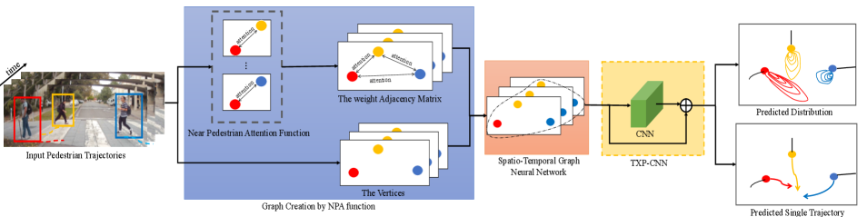
Our proposed model consists of three parts: (1) a Near Pedestrian Attention Function (NPA); (2) the Spatio-Temporal Graph Convolution Neural Network (ST-GCNN); (3) and the Time-Extrapolator Convolution Neural Network (TXP-CNN), as shown in Fig. 2.
III-B1 Graph Construction with Near Pedestrian Attention Function
For an observed sequence, we construct a graph representation of the scene using our NPA function. At each timestep, we define an undirected graph where each node represents the displacement of agent from the prior timestep, for pedestrians. Edges of the graph are represented using a weighted adjacency matrix , where each edge represents the attention between neighbours and . In this work, we assume that a pedestrian’s motion is more easily influenced by nearby neighbours, and use our NPA function to compute attention. Closer neighbours are assigned higher attention weight by softmax as Eq.1 and Eq.2 show.
| (1) | |||
| (2) |
The publicly available implementation of Social-STGCNN [14] details usage of relative velocity between neighbours as input during graph adjacency matrix creation. In this work, we demonstrate that by instead using the relative distances between neighbours, scaled using a softmax operation to represent attention, we can better represent the influence of nearby neighbours on a pedestrian during interactions.
We use the entire spatio-temporal graph across the observed time period as input to the ST-GCNN.
III-B2 Spatio-Temporal Graph Convolution Neural Network
We apply the graph spatial convolution operation, first introduced in [14], to G. This generalizes the operation of convolution from an array to graph representation, using a kernel to aggregate features across a local neighbourhood of the graph in both spatial and temporal dimensions in a similar manner as grid based CNNs. Following prior work [23] [14], we also normalize the adjacency matrix A for each timestep to allow proper feature extraction:
| (3) |
where is denoted as the diagonal node degree of at time step and I is denoted as the identity matrix. presents the normalized weight adjacency matrix at time .
The input to each layer of the ST-GCNN is described below, where V and denote the concatenations of and along the time dimension respectively, for all . The input to the first layer is V, whilst is used for all layers:
| (4) |
is a layer-specific trainable weight matrix and is the activation function.
III-B3 Time-Extrapolator Convolution Neural Network
TXP-CNN, described in [14], acts to decode the final embedded output H from ST-GCNN along the temporal dimension, allowing prediction of future pedestrian trajectories for a given time period . This module was inspired by Temporal Convolution Neural Networks (TCNs)[21] and makes use of residual layers [32]. The final output becomes predicted output , as expressed below:
| (5) | |||
| (6) |
where and represent the activation function and layer-specific trainable weight matrices respectively.
III-B4 Loss Functions
The probabilistic and deterministic versions of our model make use of different loss functions during training. is used to train a probabilistic output, minimizing the negative log-likelihood of the ground truth Y given the output distribution of the model , which is defined as:
| (7) |
We introduce to train a deterministic output, minimizing average displacement error and final displacement error of the ground truth and the predicted deterministic trajectory as shown in Eq. 8, where is a hyperparameter between .
| (8) | ||||
III-C Implementation
The model consists of 1 layer of ST-GCNN and 5 layers of TXP-CNN, where both temporal convolutions and graph convolutions use a kernel size of 3. The deterministic model and the probabilistic model both use PReLu activations [33] and are trained for 150 epochs with the batch size of 128. We use Adam optimiser [34] with learning rate at 0.0015 for training the deterministic model, however we use the SGD optimiser with learning rate at 0.01 in the training of the probabilistic model as this was seen to achieve better training results.
IV USyd Campus Pedestrian dataset
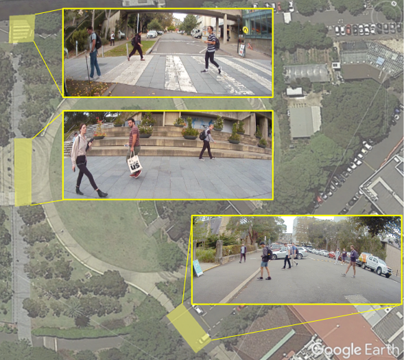
The USyd Campus Pedestrain dataset was collected at three different locations during peak times at the University of Sydney, as shown in Fig. 4 and contains more than 37 minutes in total.
IV-A Dataset Platform
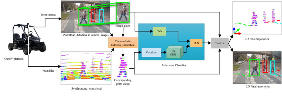
Data was captured from an Electric Vehicle (EV) platform similar to [35], as depicted in Fig 3. Sensing consists of three front NVIDIA 2Mega SF3322 automotive GMSL cameras and a 3D Velodyne Puck VLP-16 lidar. Lidar was captured at 10 Hz and RGB at 30Hz with a resolution of resolution of . In testing, we downsample the raw camera data to 10 Hz to be consistent with the lidar sample rate. 2D cameras were intrinsically calibrated based on fish-eye camera model [36] before extrinsic calibration with lidar, performed automatically using 3D point and plane correspondences, proposed by Verma et al. [37].
IV-B Automatic Labelling
The dataset was labelled using an automatic perception pipeline shown in Fig 3 based on the work proposed by [38]. This pipeline includes 2D object detection using YOLOv3 [39], a 3D lidar classification model based on [40] and [41], and a Deepsort visual tracker [42]. Each potential pedestrian image patch found by YOLOv3 is projected into the 3D pointcloud, associating it with a cluster of points that depicts the subject in the lidar pointcloud. This cluster is then voxelised and forwarded to a 3D CNN. The image patch is also passed through another CNN. Finally, the output of both convolutional pipelines are concatenated and passed to a fully connected layer that classifies the sample as either a true pedestrian or a false positive. We relied on this pipeline instead of a 2D-based one because the urban environment contains a range of objects that look like pedestrians but they are not pedestrians. For instance, we could find billboards, posters and digital displays depicting people. A 2D-based approach would eventually detect these objects as pedestrians and, thus, extracting a false positive. The original image patch is then encoded by secondary 2D CNN to extract features used by Deepsort, associating it in the 2D frame. For true pedestrians, the original image patch is then associated with prior tracks in the 2D frame using Deepsort [42], before the 3D coordinates of the pointcloud cluster are used to transform the track into the world frame. Linear interpolation is applied to allow trajectories to be continuous across short occlusions.
V Experiments
We conduct several experiments to validate our proposed probabilistic and deterministic models, comparing performance to a number of baselines using 3 real-world datasets. These include two with a top-down view; ETH [43] and UCY [24] datasets, and our proposed USyd Pedestrian Dataset collected from an intelligent vehicle reflecting a real-world vehicle sensor implementation. Additionally, we compare both parameter size and inference times for tested methods.
V-A Datasets
ETH [43] contains two scenes, ETH-Univ is collected from a University, and ETH-Hotel is collected in urban street. The dataset is converted to world coordinates with an observation frequency of 2.5 Hz.
UCY [24] includes UCY-Zara01, UCY-Zara01 and UCY-Hotel collected from an urban scene. The trajectories in the datasets are sampled every 0.4 seconds.
USyd Pedestrian Dataset is collected by a vehicle operating in a university campus as described in Sec. IV sampled at 10 Hz.
V-B Evaluation Metrics and Baselines
V-B1 Metrics
Similar to prior work [4, 2], we use Average Displacement Error (ADE) and Final Displacement Error(FDE) to evaluate the deterministic models. In evaluation of probabilistic models, we use Best-of-N (BoN) in the same manner as prior work [5] [8] [14].
The metrics used are as follows:
-
•
Average Displacement Error (ADE): Average Euclidean distance between ground truth and prediction trajectories for all predicted time steps.
-
•
Final Displacement Error (FDE): Euclidean distance between ground truth and prediction trajectories at the final predicted time step.
-
•
Best-of-N (BoN): The best sample with minimum ADE and FDE amongst N sampled trajectories from the output distribution.
V-B2 Baseline
We compare our deterministic and probabilistic model versions separately to the following baselines. We additionally compare our probabilistic model when limited to a single ‘most-likely’ prediction against all deterministic methods:
Deterministic Models:
Probalistic Models:
-
•
SocialGAN [5]: LSTM encoder-decoder with a social pooling layer, trained adversarially.
-
•
Sophie [7]: LSTM network with a proposed a physical and social attention module, trained adversarially
-
•
STSGN [9]: LSTM with graph attention network for stochastic trajectory prediction.
-
•
Social-BiGAT [10]: LSTM network with a Graph Attention Network (GAT) to encode the interaction information, trained adversarially.
-
•
Social-STGCNN [14]: Spatio-temporal graph based neural network.
V-C Methodology
For both the ETH and UCY datasets we observe the last 8 timesteps (3.2 seconds) per trajectory and predict for the next 12 timesteps (4.8 seconds). For the Usyd Pedestrian dataset, as tracks tend to be of shorter length due to occlusion from the vehicles viewpoint, we only observe 4 timesteps (0.4s) per trajectory and predict for the next timesteps (1.2 seconds). We split all datasets into training, validation and testing sets, in ratios , and respectively.
We additionally compare the parameter size and inference time of each of the predictive models, an important consideration for real-world applications of autonomous vehicles.
| Probalistics Models | (1) ADE/ FDE (m), Best of 20 Samples | |||||
|---|---|---|---|---|---|---|
| ETH-Univ | ETH-Hotel | UCY-Univ | UCY-ZARA1 | UCY-ZARA2 | Average | |
| Social GAN [5] | 0.87/1.62 | 0.67/1.37 | 0.76/1.52 | 0.35/0.68 | 0.42/0.84 | 0.61/1.21 |
| SoPhie [7] | 0.70/1.43 | 0.76/1.67 | 0.54/1.24 | 0.30/0.63 | 0.38/0.78 | 0.54/1.15 |
| Next [8] | 0.73/7.65 | 0.30/0.59 | 0.60/1.27 | 0.38/0.81 | 0.31/0.68 | 0.46/1.00 |
| STSGN [9] | 0.75/1.63 | 0.63/1.01 | 0.48/1.08 | 0.30/0.65 | 0.26/0.57 | 0.48/0.99 |
| Social-BiGAT [10] | 0.69/1.29 | 0.49/1.01 | 0.55/1.32 | 030/0.62 | 0.36/0.75 | 0.48/1.00 |
| Social-STGCNN [14] | 0.64/1.11 | 0.49/0.85 | 0.44/0.79 | 0.34/0.53 | 0.30/0.48 | 0.44/0.75 |
| Ours (probalistic model) | 0.68/1.22 | 0.31/0.41 | 0.39/0.69 | 0.34/0.55 | 0.28/0.44 | 0.40/0.66 |
| Detrministic Models | (2) ADE/ FDE (m) | |||||
| ETH-Univ | ETH-Hotel | UCY-Univ | UCY-ZARA1 | UCY-ZARA2 | Average | |
| Linear | 0.79/1.57 | 0.39/0.72 | 0.82/1.59 | 0.62/1.21 | 0.77/1.48 | 0.68/1.31 |
| CVM [44] | 0.70/1.34 | 0.33/0.62 | 0.56/1.20 | 0.46/0.99 | 0.35/0.75 | 0.48/0.98 |
| PCGAN [18] | 0.65/1.25 | 0.64/1.40 | 0.57/1.24 | 0.40/0.89 | 0.34/0.77 | 0.52/1.11 |
| SR-LSTM [2] | 0.63/1.25 | 0.37/0.74 | 0.51/1.10 | 0.41/0.90 | 0.32/0.70 | 0.45/0.94 |
| Social STGCNN (most-likely) [14] | 1.02/1.95 | 0.66/1.32 | 0.69/1.36 | 0.59/1.18 | 0.44/0.90 | 0.68/1.34 |
| Ours (probabilistic - most-likely) | 0.98/1.88 | 0.55/1.22 | 0.61/1.21 | 0.54/1.09 | 0.48/0.94 | 0.63/1.26 |
| Ours (deterministic model) | 1.0/1.8 | 0.38/0.50 | 0.6/1.14 | 0.45/0.81 | 0.36/0.66 | 0.55/0.98 |
VI Result and Discussion
VI-A Quantitative Evaluation
Probabilistic Predictions: Table II displays the comparison for all probabilistic methods on the ETH [43] and UCY [24] datasets. On average, our probabilistic model obtains better results than all other compared probabilistic models with improvement on ADE and improvement on FDE compared to the next best model Social-STGCN [14]. This result demonstrates that our proposed NPA module, which embeds relative distance based attention between pedestrians into the graph, improves performance greatly. Whilst our probabilistic model only achieves the best accuracy on 4 out of 10 individual metrics, it is clear from the average score that our approach is better able to generalise between datasets than other compared methods. Additionally, we see that both our proposed method and Social-STGCNN outperform the compared LSTM methods [8, 5, 10], demonstrating that GNN and CNN based methods can achieve significantly better results than LSTM based methods in pedestrian motion prediction tasks. It is clear from these results that the spatial-temporal graph neural network is able to successfully extract the features relevant to implicit interaction between pedestrians.
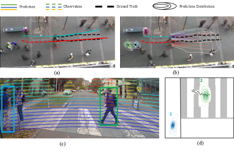
Table. III shows results from the Usyd pedestrian dataset. Our proposed probabilistic model and Social-STGCNN significantly outperform all other methods, including the probabilistic SocialGAN method, although Social-STGCNN achieves slightly better results in ADE and FDE. Due to the limited observation period of 4 timesteps, social interactions are not as prominent, and so our proposed NPA function was likely not able to better represent relationships. Additionally, significant noise exists compared to top-down datasets, as seen in the bottom right of Fig. 1. This is typical of real-world data collected from a vehicle, resulting from occlusions, sensor noise, and lidar firing cycles mismatching with 2D input. The noise is also a likely explanation for the minimal difference seen between ADE and FDE for our method and Social-STGCNN. The ground truth path contains significant noise however the predicted path directly leads to the final ground truth position, resulting in lower final but higher average error.
| USyd Pedestrian Dataset | |
|---|---|
| Linear | 0.57/0.93 |
| CVM [44] | 1.1/1.76 |
| Social GAN [5] | 1.24/2.32∗ |
| Social STGCNN [14] | 0.30/0.29∗ |
| Ours-Probabilistic | 0.32/0.31∗ |
| Ours-Deterministic | 0.46/0.84 |
| Method | Number of Parameters | Inference Time (ms) |
|---|---|---|
| S-GAN [5] | 46.6K | |
| S-P-GAN [5] | 360.3K | |
| PCGAN [4] | 66.2k | 18.63 |
| SR-LSTM [2] | 64.9K | 102.1 |
| CVM [44] | N/A | 29.45 |
| Social-STGCNN | 7.6K | |
| Ours-Probabilistic | 7.6K | |
| Ours-Deterministic | 7.6K |
Deterministic Predictions: Table. LABEL:table_deterministic shows the results of testing the deterministic models on the ETH [43] and UCY [24] datasets, displaying both our deterministic model, and our probabilistic model that has been limited to outputting a single ‘most-likely’ prediction. We see that directly training our model in a deterministic fashion as opposed to using the ‘most-likely’ prediction of the probabilistic model results in increased prediction accuracy, an important consideration in time-critical tasks where only a single prediction without uncertainty is required. Whilst SR-LSTM outperforms our deterministic model in both ADE and FDE, we see in Table. IV that SR-LSTM inference takes significantly longer, limiting the applicability for use in time-critical tasks in autonomous driving systems. CVM also achieves good results, however as described in [4] some subsets of the data used, such as ETH-Hotel, appear to involve significantly fewer pedestrian interactions suggesting that linear models should perform well. This appears to be the case when we focus on examples of pedestrian interaction from the datasets, as described in Section VI-B and shown in Fig. 5.
Computation Speed Comparison: We bench-mark inference time for 8 observed and 12 prediction timesteps running on an Nvidia GTX 1080Ti GPU and Intel Xeon E5v4 CPU in Table IV. Our proposed method and Social-STGCNN achieve the fastest computation speed among all models with the least number of parameters, suggesting that GCNN-based methods not only outperform state of the art probabilistic RNN-based methods but also requires much less computational resources. Furthermore, our approach also outperforms the CPU implemented Kalman filter based CVM method. As per [14], we do not include graph computation time due to the use of an non-optimized CPU implementation, however this process takes approximately 22ms, resulting in speeds still comparable to the next fastest PCGAN method when included. Whilst our proposed method has the same size and speed as Social-STGCNN [14], our method achieves superior performance on ADE and FDE metrics as Table II shows.
VI-B Qualitative Evaluation
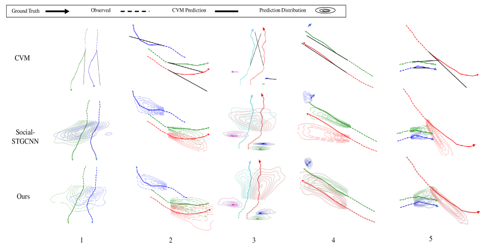
Comparisons in interactive scenarios, shown in Fig. 5, confirms the robustness of our proposed method. We compare our proposed method with Social-STGCNN [14] to demonstrate the benefit of our proposed NPA function during pedestrian encounters, and also to CVM [44] to highlight instances when linear predictions fail.
Parallel Walking Generally, when a group of pedestrians are walking in parallel, they maintain similar walking speeds and direction. As it shows in Scenario 1 of Fig. 5 in which two pedestrians walk side by side, Social-STGCNN [14] falsely predicts the pedestrians will collide with each other while our approach predicts similar distributions for each pedestrian. In Scenario 3 and Scenario 4, Social-STGCNN [14] predicts the pedestrians will begin to diverge, whilst our method predicts future trajectory distributions with the same direction and speed. We can clearly see that CVM [44] fails in the situations when pedestrians change direction, or some noise exists, as in Scenario 3.
Collision Avoidance Scenarios 4 and 5 show situations when pedestrians are approaching another stationary (4) or moving (5) pedestrian. Our proposed model predicts that both the approaching pedestrians and the stationary pedestrian will change heading slightly to avoid a collision, while Social-STGCNN falsely predicts greater incorrect deviation by approaching pedestrians. Similarly, when a single individual interacts with a group, it is difficult to predict their response, as illustrated in scenarios 2, 4, and 5. In (4), the stationary pedestrian is likely to move aside to avoid an approaching group. Our proposed method correctly predicts this motion while Social-STGCNN predicts an incorrect direction. Likewise, in (5), both CVM and Social-STGCNN [14] predict a collision, while our predicted direction better follows the ground truth response.
VII CONCLUSIONS
In this paper, we demonstrate improved probabilistic pedestrian motion prediction using our proposed graph neural network with a novel graph attention function related to the proximity between pedestrians. We also show how this same model can be trained to improve deterministic performance when only a single prediction, and no measure of uncertainty is required. This use case is especially important to time-critical tasks in autonomous vehicle applications, which we explore through a comparison of model inference speeds, highlighting the advantage of our proposed approaches. Additionally, we address the need to use training datasets representative of real-world usage, proposing an automatically labelled dataset for autonomous vehicles to verify and evaluate pedestrian motion prediction models. Our work focuses on how pedestrians interact with each other to allow vehicles to navigate safely in crowds. In the future, we will extend our work to incorporate motion prediction for heterogeneous traffic agents allowing autonomous vehicles to safely navigate in more complex driving environments.
References
- [1] A. Alahi, K. Goel, V. Ramanathan, A. Robicquet, L. Fei-Fei, and S. Savarese. Social LSTM: Human trajectory prediction in crowded spaces. In CVPR, 2016.
- [2] P. Zhang, W. Ouyang, P. Zhang, J. Xue, and N. Zheng. SR-LSTM: State Refinement for LSTM towards Pedestrian Trajectory Prediction. In CVPR, 2019.
- [3] A. Vemula, K. Muelling, and J. Oh. Social Attention : Modeling Attention in Human Crowds. In ICRA, 2018.
- [4] S. Eiffert, K. Li, M. Shan, S. Worrall, S. Sukkarieh, and E. Nebot. Probabilistic crowd gan: Multimodal pedestrian trajectory prediction using a graph vehicle-pedestrian attention network. IEEE Robotics and Automation Letters, 5(4):5026–5033, 2020.
- [5] A. Gupta, J. Johnson, L. Fei-Fei, S. Savarese, and A. Alahi. Social GAN: Socially acceptable trajectories with generative adversarial networks. In CVPR, 2018.
- [6] B. Ivanovic and M. Pavone. The Trajectron: Probabilistic Multi-Agent Trajectory Modeling With Dynamic Spatiotemporal Graphs. In ICCV, 2019.
- [7] A. Sadeghian, V. Kosaraju, A. Sadeghian, N. Hirose, S. H. Rezatofighi, and S. Savarese. SoPhie: An Attentive GAN for Predicting Paths Compliant to Social and Physical Constraints. In CVPR, 2018.
- [8] J. Liang, L. Jiang, J. C. Niebles, A. G. Hauptmann, and L. Fei-Fei. Peeking into the future: Predicting future person activities and locations in videos. In CVPR, 2019.
- [9] L. Zhang, Q. She, and P. Guo. Stochastic trajectory prediction with social graph network. arXiv preprint arXiv:1907.10233, 2019.
- [10] V. Kosaraju, A. Sadeghian, R. Martín-Martín, I. Reid, S. H. Rezatofighi, and S. Savarese. Social-BiGAT: Multimodal Trajectory Forecasting using Bicycle-GAN and Graph Attention Networks. In NeurIPS, 2019.
- [11] A. Rudenko, L. Palmieri, M. Herman, K. M. Kitani, D. M. Gavrila, and K. O. Arras. Human motion trajectory prediction: a survey. The International Journal of Robotics Research, 39(8):895–935, 2020.
- [12] S. Magdici and M. Althoff. Fail-safe motion planning of autonomous vehicles. In ITSC, 2016.
- [13] T. Salzmann, B. Ivanovic, P. Chakravarty, and M. Pavone. Trajectron++: Multi-agent generative trajectory forecasting with heterogeneous data for control. arXiv:2001.03093, 2020.
- [14] A. Mohamed, K. Qian, M. Elhoseiny, and C. Claudel. Social-stgcnn: A social spatio-temporal graph convolutional neural network for human trajectory prediction. In CVPR, pages 14424–14432, 2020.
- [15] S. Eiffert, N. Wallace, H. Kong, N. Pirmarzdashti, and S. Sukkarieh. Path Planning in Dynamic Environments using Generative RNNs and Monte Carlo Tree Search. ICRA, 2020.
- [16] J. F. Fisac, A. Bajcsy, S. L. Herbert, D. Fridovich-Keil, S. Wang, C. Tomlin, and A. D. Dragan. Probabilistically Safe Robot Planning with Confidence-Based Human Predictions. RSS, 2018.
- [17] P. Veličković, G. Cucurull, A. Casanova, A. Romero, P. Liò, and Y. Bengio. Graph Attention Networks. International Conference on Learning Representations, 2018.
- [18] S. Eiffert and S. Sukkarieh. Predicting Responses to a Robot’s Future Motion Using Generative Recurrent Neural Networks. In Australian Conference on Robotics and Automation (ACRA), 2019.
- [19] Y. Ma, X. Zhu, S. Zhang, R. Yang, W. Wang, and D. Manocha. Trafficpredict: Trajectory prediction for heterogeneous traffic-agents. In AAAI, 2019.
- [20] T. Wang, L. Liu, H. Zhang, L. Zhang, and X. Chen. Joint character-level convolutional and generative adversarial networks for text classification. Complexity, 2020.
- [21] S. Bai, J. Z. Kolter, and V. Koltun. An empirical evaluation of generic convolutional and recurrent networks for sequence modeling. arXiv preprint arXiv:1803.01271, 2018.
- [22] A. Vaswani, N. Shazeer, N. Parmar, J. Uszkoreit, L. Jones, A. N. Gomez, Ł. Kaiser, and I. Polosukhin. Attention is all you need. In Advances in neural information processing systems, 2017.
- [23] T. N. Kipf and M. Welling. Semi-supervised classification with graph convolutional networks. arXiv preprint arXiv:1609.02907, 2016.
- [24] A. Lerner, Y. Chrysanthou, and D. Lischinski. Crowds by example. In Computer graphics forum, volume 26, pages 655–664, 2007.
- [25] A. Robicquet, A. Sadeghian, A. Alahi, and S. Savarese. Learning social etiquette: Human trajectory understanding in crowded scenes. In ECCV, 2016.
- [26] D. Yang, L. Li, K. Redmill, and Ü. Özgüner. Top-view trajectories: A pedestrian dataset of vehicle-crowd interaction from controlled experiments and crowded campus. Intelligent Vehicles Symposium, 2019.
- [27] B. Benfold and I. Reid. Stable multi-target tracking in real-time surveillance video. In CVPR, 2011.
- [28] B. Zhou, X. Wang, and X. Tang. Understanding collective crowd behaviors: Learning a mixture model of dynamic pedestrian-agents. In CVPR, 2012.
- [29] P. Sun, H. Kretzschmar, X Dotiwalla, A. Chouard, V. Patnaik, P Tsui …, and D Anguelov. Scalability in perception for autonomous driving: Waymo open dataset. In CVPR, 2020.
- [30] A. Geiger, P. Lenz, and R. Urtasun. Are We Ready for Autonomous Driving? The KITTI Vision Benchmark Suite. In CVPR, 2012.
- [31] J. Houston, G. Zuidhof, L. Bergamini, Y. Ye, A. Jain, S. Omari, V. Iglovikov, and P. Ondruska. One thousand and one hours: Self-driving motion prediction dataset. arXiv preprint 2006.14480, 2020.
- [32] K. He, X. Zhang, S. Ren, and J. Sun. Deep residual learning for image recognition. In CVPR, 2016.
- [33] K. He, X. Zhang, S. Ren, and J. Sun. Delving deep into rectifiers: Surpassing human-level performance on imagenet classification. In ICCV, 2015.
- [34] D. P. Kingma and J. Ba. Adam: A method for stochastic optimization. arXiv preprint arXiv:1412.6980, 2014.
- [35] W. Zhou, J.S. Berrio Perez, C. De Alvis, M. Shan, S. Worrall, J. Ward, and E. Nebot. Developing and Testing Robust Autonomy: The USyd Campus Dataset. Intelligent Transportation Systems Magazine, 2020.
- [36] J. Kannala and S. Brandt. A generic camera calibration method for fish-eye lenses. In ICPR, 2004.
- [37] S. Verma, J.S. Berrio Perez, S. Worrall, and E. Nebot. Automatic extrinsic calibration between a camera and a 3D Lidar using 3D point and plane correspondences. In ITSC, 2019.
- [38] F. Gomez-Donoso, E. Cruz, M. Cazorla, S. Worrall, and E. Nebot. Using a 3D CNN for Rejecting False Positives on Pedestrian Detection. In IEEE International Joint Conference on Neural Networks, 2020.
- [39] J. Redmon and A. Farhadi. Yolov3: An incremental improvement. arXiv preprint arXiv:1804.02767, 2018.
- [40] A. Garcia-Garcia, F. Gomez-Donoso, J. Garcia-Rodriguez, S. Orts-Escolano, M. Cazorla, and J. Azorin-Lopez. Pointnet: A 3D convolutional neural network for real-time object class recognition. In IEEE International Joint Conference on Neural Networks, 2016.
- [41] F. Gomez-Donoso, F. Escalona, and M. Cazorla. Par3dnet: Using 3dcnns for object recognition on tridimensional partial views. Applied Sciences, 10(10):3409, May 2020.
- [42] N. Wojke, A. Bewley, and D. Paulus. Simple online and realtime tracking with a deep association metric. In IEEE International Conference on Image Processing (ICIP), 2017.
- [43] S. Pellegrini, A. Ess, K. Schindler, and L. Van Gool. You’ll never walk alone: Modeling social behavior for multi-target tracking. In ICCV, 2009.
- [44] C. Schöller, V. Aravantinos, F. Lay, and A. Knoll. What the Constant Velocity Model Can Teach Us About Pedestrian Motion Prediction. ICRA, 2020.