Attention Guided CAM:
Visual Explanations of Vision Transformer Guided by Self-Attention
Abstract
Vision Transformer(ViT) is one of the most widely used models in the computer vision field with its great performance on various tasks. In order to fully utilize the ViT-based architecture in various applications, proper visualization methods with a decent localization performance are necessary, but these methods employed in CNN-based models are still not available in ViT due to its unique structure. In this work, we propose an attention-guided visualization method applied to ViT that provides a high-level semantic explanation for its decision. Our method selectively aggregates the gradients directly propagated from the classification output to each self-attention, collecting the contribution of image features extracted from each location of the input image. These gradients are additionally guided by the normalized self-attention scores, which are the pairwise patch correlation scores. They are used to supplement the gradients on the patch-level context information efficiently detected by the self-attention mechanism. This approach of our method provides elaborate high-level semantic explanations with great localization performance only with the class labels. As a result, our method outperforms the previous leading explainability methods of ViT in the weakly-supervised localization task and presents great capability in capturing the full instances of the target class object. Meanwhile, our method provides a visualization that faithfully explains the model, which is demonstrated in the perturbation comparison test.
Introduction
Transformer-based models (Vaswani et al. 2017; Devlin et al. 2018; Liu et al. 2019; Radford et al. 2018) is a widely used architecture in various NLP tasks due to its superior performance. Vision Transformer (ViT) (Dosovitskiy et al. 2020) is a modified Transformer that adopts the architecture of BERT (Devlin et al. 2018), but is applicable to images by replacing its basic unit of operation with image patches. As a Transformer-based model, ViT applies the self-attention mechanism as its primary operation, sharing the advantages of the Transformer over other models: it significantly reduces the required computational load and supports better parallelization. Furthermore, recent studies propose that ViT is better at shape recognition (Tuli et al. 2021) and shows high robustness against occlusions and perturbations in the input (Naseer et al. 2021). Exploiting these benefits, ViT and its derived models have achieved remarkable performance in numerous vision tasks such as classification (Chen, Fan, and Panda 2021; Li et al. 2021; Touvron et al. 2021), object detection (Liu et al. 2021; Wang et al. 2021), and semantic segmentation (Ranftl, Bochkovskiy, and Koltun 2021; Zheng et al. 2021). Demonstrating its high versatility and decent performance, especially in large-scale image data, it is now considered as a practical alternative to Convolutional Neural Network (CNN) (He et al. 2016; LeCun et al. 1989; Simonyan and Zisserman 2014; Szegedy et al. 2015) which has dominated the computer vision field for the past decade.
Despite the notable success of ViT in computer vision, it still lacks explainability. The proper methods to provide a visual explanation of the model are vital to ensure the reliability of the given model. For CNN, for example, numerous methods have been developed to provide a faithful explanation of the model by gradient analysis (Draelos and Carin 2020; Selvaraju et al. 2017; Zhou et al. 2016). In addition, many of the gradient-based methods have been actively utilized in weakly-supervised localization (Chattopadhay et al. 2018; Qin, Kim, and Gedeon 2021; Yang et al. 2020). In contrast, the unique structure of ViT, such as the use of token and the self-attention mechanism, makes it complicated to provide the proper explanation of the model. Therefore, compared to CNN, there have been fewer explainability methods developed, including Attention rollout (Abnar and Zuidema 2020) and Layer-wise Relevance Propagation (LRP)-based method (Chefer, Gur, and Wolf 2021).
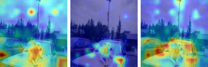
Attention Rollout is a method developed for ViT and aims to provide a concise aggregation of the overall attention by using the resulting matrix of self-attention operation. Although it considers the core component of ViT architecture, it assumes a linear combination of attention and overlooks the influence of the MLP head, resulting in a rough and non-class-specific explanation of the classification decision. On the other hand, the LRP-based method applied to ViT provides a class-specific analysis and takes the whole model into consideration. It focuses on decomposing the model back into the level of image patches and calculates the relevancy score of each patch based on the conservation property. Since both methods take the self-attention operation into account, they are prone to the peak intensity resulting from the repeated softmax operation in the sequential self-attention module. The softmax operation tends to amplify the local large values in the process of converting the self-attention scores into probabilities. Consequently, it generates a peak intensity that highlights the specific point of a homogeneous background of the input image due to high self-attention scores from similar pixel intensities. As demonstrated in Figure 1, Attention Rollout and LRP-based method are severely influenced by the peak intensity, resulting in poor localization performance. In contrast, our method renormalizes the self-attention scores with sigmoid, which does not affect the original prediction process, and therefore is much less disturbed by the peak intensity.
In this work, we propose an attention-guided gradient analysis that aims to improve localization performance by combining the essential target gradients with the feedforward feature of the self-attention module. Specifically, to provide the class activation map (CAM) of high-semantic explanation, we aggregate the gradients that are directly connected to the MLP head and backpropagated along skip connections. Also, we conclude that the self-attention score represents the patch correlation scores with a continuous pattern and preserves spatial position information. Therefore, we use the self-attention score, which is newly normalized with the sigmoid operation to alleviate peak intensities, as feature maps that guide the gradients on the pattern information of the image. In short, the proposed method provides the CAM that represents the image features of the input combined with their contributions to the prediction of the model. This approach achieves greater weakly-supervised localization performance with the state-of-the-art result in most evaluation benchmarks. The contributions of this work are as follows:
-
•
We propose a gradient-based method applicable to Vision Transformer that fully considers the major structures of the model and provides a reliable high-semantic explanation of the model.
-
•
The proposed method aggregates the selective gradients guided by the self-attention to construct a class activation map (CAM) of great localization performance.
-
•
Our method outperforms the previous leading methods applied to ViT in the experiments on weakly-supervised localization. We also demonstrate the improved reliability of our method by pixel perturbation experiment.
| Raw Attention | Attention Rollout | LRP-based | Ours |


Related Works
Explainability of a deep neural network matters because the black box nature of it makes it difficult to ensure that the model is working in a proper way. Hence, there have been various methods that aim to explain the model’s inner workings, but each method adopts a different idea of what it intends to explain and how it generates the explanations. For example, in Attention Rollout (Abnar and Zuidema 2020) which is designed to explain the Transformer, the explanation means the amount of information propagated from the first to the last self-attention module. Although it can be easily applied to any Transformer-based model, it does not take the MLP heads into account and cannot specify how much each captured correlation contributes to the classification output of a particular class. Therefore, Attention Rollout produces a non-class-specific explanation and shows lower performance in localization tasks for some regions that are unrelated to the classification output are also highlighted.
LRP-based methods are contrived to calculate the relevancy score of the input pixel to the classification output. In other words, the explanation provided by LRP is the contribution of each pixel of the input image throughout the model from the input to the output. It first decomposes a model pixel-wisely typically using Deep Taylor Decomposition (DTD) framework (Montavon et al. 2017), then it calculates the relevancy of each of the pixels by propagating the decomposed relevancies backward from the output to the input layer. LRP-based methods have been extended to various models. Bach et al., (Bach et al. 2015) proposed an LRP method that can consider the nonlinearity of the model, and Binder et al., (Binder et al. 2016a) applied LRP to some deep neural networks including GoogLeNet and VGG. They, then, extend LRP to the renormalization layer (Binder et al. 2016b). Finally, Chefer et al., (Chefer, Gur, and Wolf 2021) introduced the LRP-based method applied to ViT by proposing the method to apply LRP to the GELU (Hendrycks and Gimpel 2016) layer, skip connections, and matrix multiplication, which are the major operations of ViT and calculates the relevancy score of each image patch. These methods capture the contribution of each independent and discrete unit of the model and provide a precise explanation. However, they often result in scattered contributions which only highlight a partial area of the target class object because of approximation error in relevancy calculation and incomplete attention scores as shown in Figure 1.

On the other hand, the gradient-based methods provide a high-semantic explanation of the model, meaning that they explain the contribution of the image features elicited through multiple layers, rather than the contribution of the independent pixels. The earliest gradient-based method is Class Activation Map (CAM) (Zhou et al. 2016), which generates a saliency map as a result of the weighted sum of the feature map channels of the last convolutional layer. Here, the weights for each feature map channel are calculated by a single time backward from the classification output of the target class. Grad-CAM (Selvaraju et al. 2017) proposes a generalized CAM, whose usage is not restricted to a model with Global Average Pooling (GAP). Grad-CAM averages the gradients of each channel to construct a class activation map of a general CNN model with fully connected layers. HiResCAM (Draelos and Carin 2020) provides a more faithful explanation by replacing the channel-wise weights of the Grad-CAM with the pixel-wise multiplication of the gradients and the feature maps. Gradient-based methods are also highly utilized in weakly-supervised object localization with great performance. Grad-CAM++ (Chattopadhay et al. 2018) proposed a generalized version of Grad-CAM with improved localization performance, adding channel-wise weights to the Grad-CAM. Combinational CAM (Yang et al. 2020) and infoCAM (Qin, Kim, and Gedeon 2021) integrate the CAM of non-label classes to localize the target object more precisely. In these gradient-based methods, the feature maps reflect the interaction among the pixels from multiple layers of the model and the gradients are the contributions of these high-level image features. This approach of the gradient-based methods that combines the feature maps and their gradients intrinsically results in a continuous heatmap where contributions cluster together on the target object and also gives an excellent capability in object localization.
Methodology
Our method applies the gradient-based visualization technique to ViT (Dosovitskiy et al. 2020) to generate the class activation map (CAM) (Zhou et al. 2016; Selvaraju et al. 2017) of the target class. The major components of our method are demonstrated in Figure 2. To generate a high-semantic explanation of the model, we focus on the gradients from the classification output to each encoder block along the backward path through the skip connection. In addition, these essential gradients are guided by feature maps obtained from the newly normalized self-attention score matrices by sigmoid. The reasons why the gradients and the feature map are obtained from the self-attention blocks are as follows. Firstly, the attention score matrice at each block contains the high-level image features elicited through the self-attention mechanism. Given that these image features represent pairwise patch correlations, these matrices are appropriate to be used as a feature map. Secondly, regardless of the aggregation option chosen in the MLP head (e.g. token or average pooling), these matrices preserve the patch position information of the input image. Here in this paper, we explain our method based on the original ViT model with a token.
According to the ViT architecture, the input with a size of is flattened and converted into a patch embedding with a size of before fed into the transformer encoder. Here, the number of patches equals with image patches and 1 additional for token, and the patch embedding size can vary but is generally defined as . The order of the patches embedded in this process is maintained and therefore the positional information of the image patches is traceable throughout the feedforward encoder block.
ViT architecture can be largely divided into the MLP head and the encoder blocks which consist of the self-attention, MLP, and skip connections. The patch embedding shape of is maintained at every skip connection layer and we denote this matrix after the first skip connection in the encoder block as and the one after the second skip connection in the encoder block as , respectively. During the multi-head self-attention operation in the encoder, the matrix multiplication of the query and the key matrices results in the self-attention score matrices with the size of where is the number of heads, and we denote the self-attention matrix of head as . At the end of the encoder, the MLP head produces the classification outputs and we denote the classification output of the target class as . These matrices in the ViT feedforward network and their notations are demonstrated in Figure 2.
|
softmax |

|
|
sigmoid |

|
As the feature map for gradient calculation, the self-attention matrices are used. Each element of the matrices represents the pairwise patch correlation scores detected at each layer and head and can guide the combined gradients on meaningful pattern information. Basically, in ViT, the self-attention scores are converted into the probability by the softmax operation. However, softmax tends to maximize the local large values and generates some peak intensity that suppresses other important values as shown in Figure 3. Therefore, instead of softmax, we normalize the self-attention matrices with sigmoid, which is a monotonically increasing function as well as softmax. When we denote the softmax function as and sigmoid function as , the two function satisfies the following relation:
| (1) |
At the same time, the sigmoid effectively recovers the medium correlations that are lost in softmax. The effect of replacing softmax with sigmoid is represented in Figure 3. To prevent misunderstanding, we clarify that normalization with sigmoid does not affect any backpropagation process of the original ViT structure, and sigmoid of is calculated after the model finishes learning.
Note that in ViT with token, only the first rows of , and (i.e., , and , respectively) are considered. The MLP head is only connected with the token at the end of the last encoder block, , which does not contain the positional information of the image patches itself. However, the positional information connected to this token can be traced back to the first rows of the self-attention matrices s since all operations from s along the skip connections are applied row-wisely where stands for row component. Also due to the skip connection, the MLP head is directly connected not only to in the last encoder block but also to all s in the previous blocks, as shown in Figure 2. Therefore, the feature map in our method consists of the first-row components of s normalized with sigmoid operation and is defined as:
| (2) |
The feature maps s are generated in the green boxes in Figure 2.
To produce a complete CAM, the gradients, which represent the influence of s of each block, should be combined with the feature maps. In the encoder block except for the last encoder block (i.e., , ), the gradient directly connected from the MLP head towards is propagated along the first skip connection in the block towards . By doing so, the gradient from the MLP head can be propagated to as well as to . The skip connection consists of a residual operation, a simple addition of two matrices, with no effect on the gradient passing through it. Therefore, for the first skip connection in the encoder block connected to , we get the mathematical relation as follows:
| (3) |
Then let us denote the gradient propagated from the output to the matrix in the encoder block along the skip connection path as . The gradient is defined as:
| (4) |
From Eqs. 3 and 4, we can get:
| (5) |
Since the self-attention matrices pass through a softmax layer in each block, the gradients that are propagated to each feature map are defined as:
| (6) |
However, the gradients still cause the peak-amplification effect since they contain the weights propagated from softmax. In other words, the peak amplification effect occurs due to large elements in . However, if the general attention scores are assumed to have a smooth varying property (i.e., ), the gradients propagated to each approximate the gradients propagated to each , which can be formulated as:
| (7) |
and it is proved in the supplementary material. Due to Equation 7, our method still faithfully explains the model. The final gradients are demonstrated in the yellow-shaded line in Figure 2.

Finally, the class activation map of the given class can be formulated as:
| (8) |
where refers to the Hadamard product. Here, we apply the ReLU operation on the computed gradient to reflect only the positive contribution to the classification output. Also, the contributions obtained at each location of the patch from all layers and heads are summed to combine them in the same way as the feedforward network fuses the embedded patches at each skip connection. The result of this process, , is a matrix where each value represents the contribution of each patch to the classification output of the given class . However, the first element of this matrix represents the contribution of the token which does not contain any spatial information. Since we are only interested in the contribution of each image patch, we discard the first element and construct the class activation map (CAM) with the last elements. To visualize the final CAM, the elements are reshaped to a two-dimensional image, which has the size of as demonstrated in Figure. 4. Then it is interpolated to have the same size as the input image and eventually generates the final CAM of the model.
Experiments
In this section, we present the results of the performance comparison of our method with previous leading methods. The compared methods here are the current explainability methods devised for ViT that consist of Attention Rollout (Abnar and Zuidema 2020) and LRP-based method for ViT (Chefer, Gur, and Wolf 2021).
Experimental Setup
Datasets and Evaluation Metrics. For the evaluation, we used the validation set of ImageNet ILSVRC 2012 (Russakovsky et al. 2015) and Pascal VOC 2012 (Everingham et al. 2012) and the test set of Caltech-UCSD Birds-200-2011 (CUB 200) (Wah et al. 2011), which provide the bounding-box annotation label. In quantitative evaluation, the images with more than one class label in PASCAL VOC 2012 are excluded and only single-class images are used. During the weakly-supervised localization evaluation, the input images for which the model produces a wrong prediction are excluded since the heatmaps are not reliable in this case.
For the weakly-supervised localization test, the performance is measured by pixel accuracy, Intersection over Union (IoU), Dice coefficient (F1), precision, and recall scores. The pixel perturbation test is measured by the ABPC score (Samek et al. 2016) with pixel-level perturbation. The ABPC score is the area between the LeRF and MoRF perturbation curves where the LeRF curve removes the least relevant pixels first and the MoRF curve removes the most relevant pixels first. A larger ABPC value indicates a better quality of the heatmap.
Implementation Details. All methods are evaluated with the same ViT-base (Dosovitskiy et al. 2020) model that takes the input image with a size of . All methods share the same model parameters and the fine-tuning details of the model parameters are provided in the supplementary material. In this ViT, the input images are converted into number of patches and therefore each method generates a heatmap with a size of where one pixel corresponds to the contribution of one image patch of the input image. Before evaluation, the heatmaps are all resized into and adjusted to a min-max normalization. For the weakly-supervised object detection, we get a binary mask from the generated heatmap by applying a threshold () and then generate bounding boxes from the group of pixels that have a continuous contour. The perturbation test is applied to the ground-truth class to compare the heatmap quality on the existing object.
Results
Here we demonstrate the visualization of the heatmaps generated by all three methods. Then, we present the quantitative evaluation of each method measured by the weakly-supervised object detection metrics and pixel-perturbation.
| ImageNet ILSVRC 2012 | Pascal VOC 2012 | CUB 200 | |
|
Bounding Box |

|

|

|
|
Attention Rollout |

|

|

|
|
LRP-based |

|

|

|
|
Ours |

|

|

|
| Attention Rollout | LRP-based | Ours |
| Cat |

|
| Person |

|
| Car |
|
| Dog |

|
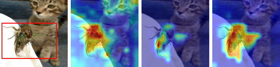
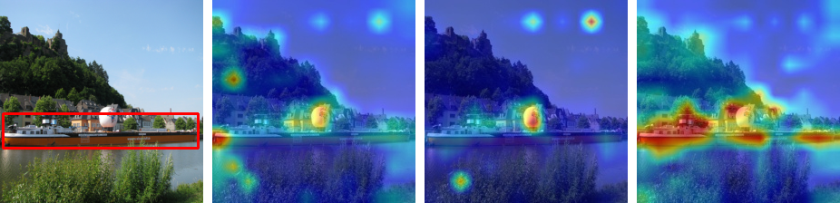
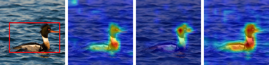
Visualization. The visualization results of each method on three datasets are presented in Figure 5. The first images of each dataset demonstrate that our method greatly improves object localization performance by successfully shading the peak intensities. As can be seen, the visualization results of the Attention Rollout and LRP-based method on the images are dominated by the peak intensities and therefore fail to localize the target objects which are indicated by the bounding boxes. Also, this result shows that our method captures the object region more precisely compared to Attention Rollout (Abnar and Zuidema 2020). Since Attention Rollout produces a non-class-specific explanation, it often highlights some unrelated background regions whereas our method successfully separates the foreground object from the background. Also, our method shows a strong point in encompassing the full object area compared to the LRP-based method (Chefer, Gur, and Wolf 2021). The LRP-based method tends to highlight a small conspicuous part of the object. Furthermore, it often misses some instances of the object in an image with multiple instances of the class object. In contrast, our method successfully localizes the whole object and also captures all the instances of the class object even when the instances are placed far from each other.
In addition, ours can also provide class-specific explanations for different classes presented within an image. Figure 6 demonstrates the results of the explanation with different target classes generated by each method. Attention Rollout does not provide a class-specific explanation and therefore produces the same results regardless of the target class label. In contrast, LRP and ours are both capable of providing a class-specific explanation of the given model. Here, our method still maintains better localization performance by fully capturing the object of each target class. The visualization results on more image samples are presented in the supplementary material.
Weakly-Supervised Object Detection. The result of the weakly-supervised object detection on the ImageNet ILSVRC 2012 validation set is presented in Table 1. This result shows that ours achieves 73.41% in pixel accuracy, 52.12% in IoU score, and 65.15% in dice coefficient, which is the highest among the three methods. Although there was a drop in precision compared to LRP-based (82.99% vs 91.10%), ours achieves a much better recall score (62.76% vs 21.76%) which is generally a trade-off with precision.
| Attention Rollout | LRP-based | Ours | |
| pixel accuracy | 0.6209 | 0.5863 | 0.7341 |
| IoU | 0.3597 | 0.2029 | 0.5212 |
| dice (F1) | 0.4893 | 0.3055 | 0.6515 |
| precision | 0.7326 | 0.9110 | 0.8299 |
| recall | 0.4657 | 0.2176 | 0.6276 |
| Attention Rollout | LRP-based | Ours | |
| pixel accuracy | 0.5592 | 0.5750 | 0.7521 |
| IoU | 0.1645 | 0.1574 | 0.5335 |
| dice (F1) | 0.2431 | 0.2348 | 0.6646 |
| precision | 0.5802 | 0.7651 | 0.8167 |
| recall | 0.2115 | 0.1716 | 0.6647 |
| Attention Rollout | LRP-based | Ours | |
| pixel accuracy | 0.7273 | 0.7039 | 0.8351 |
| IoU | 0.3097 | 0.1997 | 0.5836 |
| dice (F1) | 0.4339 | 0.3106 | 0.7220 |
| precision | 0.8357 | 0.9669 | 0.8987 |
| recall | 0.3420 | 0.1992 | 0.6438 |
| Attention Rollout | LRP-based | Ours | |
| LeRF | 0.4739 | 0.5140 | 0.5298 |
| MoRF | 0.2053 | 0.1736 | 0.1607 |
| ABPC | 0.2685 | 0.3404 | 0.3691 |
The localization performance on the Pascal VOC 2012 validation is presented in Table 2. Our method achieves 75.21% in pixel accuracy, 53.35% in IoU, and 66.46% in dice coefficient, presenting outstanding localization performance. In this case, our method also achieves the highest precision score of 81.67%.
Table 3 shows the localization performance evaluated on the test set of CUB 200. The CUB 200 dataset consists of images with a single bird per image which are easily distinguishable from the background. Therefore, patch-correlation information of the self-attention scores serves a significant role in this dataset. Our method effectively utilizes the self-attention scores, resulting in a more accurate and precise explanation compared to others, achieving 83.51% in pixel accuracy, 58.36% in IoU, and 72.20% in dice coefficient. This is about 10.78%, 27.39%, and 28.81% higher scores respectively than those of Attention Rollout.
In conclusion, our method provides a high-semantic explanation of ViT that consistently shows an outstanding performance in the weakly-supervised object detection task compared to the Attention rollout and LRP-based method. Our method shows significant improvements in terms of pixel accuracy, IoU, recall, and dice coefficient, while it still maintains an acceptable level of precision.
Pixel Perturbation. The result of the pixel perturbation test is presented in Table 4. LeRF and MoRF represent the areas under the prediction probability score curve when removing the least relevant pixels first and the most relevant pixels first, respectively. The ABPC is the area between these two curves, which is obtained by subtracting the AUC of the MoRF curve from that of the LeRF curve. Our method achieves a better LeRF score and MoRF score and therefore a higher ABPC score compared to the LRP-based method (36.91 % vs 34.04 %). This guarantees the better faithfulness and reliability of the explanations that our method provides. Additional evaluation results of the object localization task and the pixel perturbation test are presented in the supplementary materials.
Conclusion
In this work, we propose an attention-guided gradient analysis method that aims at achieving greater weakly-supervised localization performance. To this end, our method provides a high-level semantic explanation by selectively collecting the essential gradients propagated from the classification output of the target class to each self-attention matrix along the skip connection path. To supplement the gradient information with the patch correlation information that indicates the group of patches with contiguous patterns, the self-attention scores are combined with the gradients as feature maps. Before these two major components are aggregated, the self-attention scores are adapted in a way that decreases the effect of peak intensities to improve the localization performance of the CAM. As a result, our method outperforms the current state-of-the-art visualization techniques of ViT by localizing the full areas of the target object, and it especially achieves a great performance improvement in capturing the multiple instances of the given class object. This provides a reliable explanation of the model and weakly-supervised object detection method at the same time and allows ViT to be more adaptable to many tasks involving object localization in the computer vision field.
Acknowledgments
This work was supported by KIST Institutional Programs (2V09831, 2E32341, and 2E32211).
References
- Abnar and Zuidema (2020) Abnar, S.; and Zuidema, W. 2020. Quantifying attention flow in transformers. arXiv preprint arXiv:2005.00928.
- Bach et al. (2015) Bach, S.; Binder, A.; Montavon, G.; Klauschen, F.; Müller, K.-R.; and Samek, W. 2015. On pixel-wise explanations for non-linear classifier decisions by layer-wise relevance propagation. PloS one, 10(7): e0130140.
- Binder et al. (2016a) Binder, A.; Bach, S.; Montavon, G.; Müller, K.-R.; and Samek, W. 2016a. Layer-wise relevance propagation for deep neural network architectures. In Information science and applications (ICISA) 2016, 913–922. Springer.
- Binder et al. (2016b) Binder, A.; Montavon, G.; Lapuschkin, S.; Müller, K.-R.; and Samek, W. 2016b. Layer-wise relevance propagation for neural networks with local renormalization layers. In Artificial Neural Networks and Machine Learning–ICANN 2016: 25th International Conference on Artificial Neural Networks, Barcelona, Spain, September 6-9, 2016, Proceedings, Part II 25, 63–71. Springer.
- Chattopadhay et al. (2018) Chattopadhay, A.; Sarkar, A.; Howlader, P.; and Balasubramanian, V. N. 2018. Grad-cam++: Generalized gradient-based visual explanations for deep convolutional networks. In 2018 IEEE winter conference on applications of computer vision (WACV), 839–847. IEEE.
- Chefer, Gur, and Wolf (2021) Chefer, H.; Gur, S.; and Wolf, L. 2021. Transformer interpretability beyond attention visualization. In Proceedings of the IEEE/CVF Conference on Computer Vision and Pattern Recognition, 782–791.
- Chen, Fan, and Panda (2021) Chen, C.-F. R.; Fan, Q.; and Panda, R. 2021. Crossvit: Cross-attention multi-scale vision transformer for image classification. In Proceedings of the IEEE/CVF international conference on computer vision, 357–366.
- Devlin et al. (2018) Devlin, J.; Chang, M.-W.; Lee, K.; and Toutanova, K. 2018. Bert: Pre-training of deep bidirectional transformers for language understanding. arXiv preprint arXiv:1810.04805.
- Dosovitskiy et al. (2020) Dosovitskiy, A.; Beyer, L.; Kolesnikov, A.; Weissenborn, D.; Zhai, X.; Unterthiner, T.; Dehghani, M.; Minderer, M.; Heigold, G.; Gelly, S.; et al. 2020. An image is worth 16x16 words: Transformers for image recognition at scale. arXiv preprint arXiv:2010.11929.
- Draelos and Carin (2020) Draelos, R. L.; and Carin, L. 2020. Hirescam: Faithful location representation in visual attention for explainable 3d medical image classification. arXiv preprint arXiv:2011.08891.
- Everingham et al. (2012) Everingham, M.; Van Gool, L.; Williams, C. K. I.; Winn, J.; and Zisserman, A. 2012. The PASCAL Visual Object Classes Challenge 2012 (VOC2012) Results. http://www.pascal-network.org/challenges/VOC/voc2012/workshop/index.html.
- He et al. (2016) He, K.; Zhang, X.; Ren, S.; and Sun, J. 2016. Deep residual learning for image recognition. In Proceedings of the IEEE conference on computer vision and pattern recognition, 770–778.
- Hendrycks and Gimpel (2016) Hendrycks, D.; and Gimpel, K. 2016. Gaussian error linear units (gelus). arXiv preprint arXiv:1606.08415.
- LeCun et al. (1989) LeCun, Y.; Boser, B.; Denker, J. S.; Henderson, D.; Howard, R. E.; Hubbard, W.; and Jackel, L. D. 1989. Backpropagation applied to handwritten zip code recognition. Neural computation, 1(4): 541–551.
- Li et al. (2021) Li, Y.; Zhang, K.; Cao, J.; Timofte, R.; and Van Gool, L. 2021. Localvit: Bringing locality to vision transformers. arXiv preprint arXiv:2104.05707.
- Liu et al. (2019) Liu, Y.; Ott, M.; Goyal, N.; Du, J.; Joshi, M.; Chen, D.; Levy, O.; Lewis, M.; Zettlemoyer, L.; and Stoyanov, V. 2019. Roberta: A robustly optimized bert pretraining approach. arXiv preprint arXiv:1907.11692.
- Liu et al. (2021) Liu, Z.; Lin, Y.; Cao, Y.; Hu, H.; Wei, Y.; Zhang, Z.; Lin, S.; and Guo, B. 2021. Swin transformer: Hierarchical vision transformer using shifted windows. In Proceedings of the IEEE/CVF international conference on computer vision, 10012–10022.
- Montavon et al. (2017) Montavon, G.; Lapuschkin, S.; Binder, A.; Samek, W.; and Müller, K.-R. 2017. Explaining nonlinear classification decisions with deep taylor decomposition. Pattern recognition, 65: 211–222.
- Naseer et al. (2021) Naseer, M. M.; Ranasinghe, K.; Khan, S. H.; Hayat, M.; Shahbaz Khan, F.; and Yang, M.-H. 2021. Intriguing properties of vision transformers. Advances in Neural Information Processing Systems, 34: 23296–23308.
- Qin, Kim, and Gedeon (2021) Qin, Z.; Kim, D.; and Gedeon, T. 2021. Informative Class Activation Maps. arXiv preprint arXiv:2106.10472.
- Radford et al. (2018) Radford, A.; Narasimhan, K.; Salimans, T.; Sutskever, I.; et al. 2018. Improving language understanding by generative pre-training.
- Ranftl, Bochkovskiy, and Koltun (2021) Ranftl, R.; Bochkovskiy, A.; and Koltun, V. 2021. Vision transformers for dense prediction. In Proceedings of the IEEE/CVF International Conference on Computer Vision, 12179–12188.
- Russakovsky et al. (2015) Russakovsky, O.; Deng, J.; Su, H.; Krause, J.; Satheesh, S.; Ma, S.; Huang, Z.; Karpathy, A.; Khosla, A.; Bernstein, M.; Berg, A. C.; and Fei-Fei, L. 2015. ImageNet Large Scale Visual Recognition Challenge. International Journal of Computer Vision (IJCV), 115(3): 211–252.
- Samek et al. (2016) Samek, W.; Binder, A.; Montavon, G.; Lapuschkin, S.; and Müller, K.-R. 2016. Evaluating the visualization of what a deep neural network has learned. IEEE transactions on neural networks and learning systems, 28(11): 2660–2673.
- Selvaraju et al. (2017) Selvaraju, R. R.; Cogswell, M.; Das, A.; Vedantam, R.; Parikh, D.; and Batra, D. 2017. Grad-CAM: Visual Explanations From Deep Networks via Gradient-Based Localization. In Proceedings of the IEEE International Conference on Computer Vision (ICCV).
- Simonyan and Zisserman (2014) Simonyan, K.; and Zisserman, A. 2014. Very deep convolutional networks for large-scale image recognition. arXiv preprint arXiv:1409.1556.
- Szegedy et al. (2015) Szegedy, C.; Liu, W.; Jia, Y.; Sermanet, P.; Reed, S.; Anguelov, D.; Erhan, D.; Vanhoucke, V.; and Rabinovich, A. 2015. Going deeper with convolutions. In Proceedings of the IEEE conference on computer vision and pattern recognition, 1–9.
- Touvron et al. (2021) Touvron, H.; Cord, M.; Douze, M.; Massa, F.; Sablayrolles, A.; and Jégou, H. 2021. Training data-efficient image transformers & distillation through attention. In International conference on machine learning, 10347–10357. PMLR.
- Tuli et al. (2021) Tuli, S.; Dasgupta, I.; Grant, E.; and Griffiths, T. L. 2021. Are convolutional neural networks or transformers more like human vision? arXiv preprint arXiv:2105.07197.
- Vaswani et al. (2017) Vaswani, A.; Shazeer, N.; Parmar, N.; Uszkoreit, J.; Jones, L.; Gomez, A. N.; Kaiser, Ł.; and Polosukhin, I. 2017. Attention is all you need. Advances in neural information processing systems, 30.
- Voita et al. (2019) Voita, E.; Talbot, D.; Moiseev, F.; Sennrich, R.; and Titov, I. 2019. Analyzing multi-head self-attention: Specialized heads do the heavy lifting, the rest can be pruned. arXiv preprint arXiv:1905.09418.
- Wah et al. (2011) Wah, C.; Branson, S.; Welinder, P.; Perona, P.; and Belongie, S. 2011. The Caltech-UCSD Birds-200-2011 Dataset. Technical Report CNS-TR-2011-001, California Institute of Technology.
- Wang et al. (2021) Wang, W.; Xie, E.; Li, X.; Fan, D.-P.; Song, K.; Liang, D.; Lu, T.; Luo, P.; and Shao, L. 2021. Pyramid Vision Transformer: A Versatile Backbone for Dense Prediction Without Convolutions. In Proceedings of the IEEE/CVF International Conference on Computer Vision (ICCV), 568–578.
- Wightman (2019) Wightman, R. 2019. PyTorch Image Models. https://github.com/rwightman/pytorch-image-models.
- Yang et al. (2020) Yang, S.; Kim, Y.; Kim, Y.; and Kim, C. 2020. Combinational class activation maps for weakly supervised object localization. In Proceedings of the IEEE/CVF Winter Conference on Applications of Computer Vision, 2941–2949.
- Zheng et al. (2021) Zheng, S.; Lu, J.; Zhao, H.; Zhu, X.; Luo, Z.; Wang, Y.; Fu, Y.; Feng, J.; Xiang, T.; Torr, P. H.; et al. 2021. Rethinking semantic segmentation from a sequence-to-sequence perspective with transformers. In Proceedings of the IEEE/CVF conference on computer vision and pattern recognition, 6881–6890.
- Zhou et al. (2016) Zhou, B.; Khosla, A.; Lapedriza, A.; Oliva, A.; and Torralba, A. 2016. Learning deep features for discriminative localization. In Proceedings of the IEEE conference on computer vision and pattern recognition, 2921–2929.
Supplementary Materials
Supplementary Proof
Here, we prove that the gradient considered in our method, , is the approximation of the gradient propagated to the feature map, . Let us denote the softmax function as and the sigmoid function as . Then, the gradient to the original feature map, , is defined as:
| (9) |
when we denote the gradients to the matrices at the first skip connection at each encoder block, , as and the first-row self-attention score component in this block as . As stated in the methodology section, the gradients include the peak-amplification from softmax due to the last term, . Therefore, we redefine the gradient in our method in a way that avoids the peak-amplification effect as follows:
| (10) |
Despite the adaptation in the gradients, the difference between the two gradients, and is trivial. According to the chain rule, the gradient can be rewritten as follows:
| (11) |
Let us denote the element that constitutes as , and the softmax function on this vector as . Then we can write the softmax function on the vector as follows:
| (12) |
The derivative of can be written as follows:
| (13) |
When the sigmoid operation is also applied on the same sized vector and we denote the sigmoid function on this vector as , the derivative of the can be written as follows:
| (14) |
Then, the latter term of Equation 11 can be written as follows:
| (15) |
This matrix can be approximated to a diagonal matrix since
| (16) |
Let us denote the element of as and the element of as . Then, from Equation 11 and the diagonal matrix in Equation 15, can be rewritten as follows:
| (17) |
Then, we can specify the latter term in Equation 17 as the factor that amplifies the peak intensities. When we assume that the self-attention scores on general images have the smooth varying property like power law (power), we can assume the following equation:
| (18) |
Due to Equation 18, the follow relationship is satisfied:
| (19) |
and therefore the gradients of our method still faithfully explain the contribution of each patch in the feature map .
| raw attention | Grad-CAM | full-LRP | partial-LRP | Ours | |
| pixel accuracy | 0.5079 | 0.5138 | 0.4994 | 0.5959 | 0.7341 |
| IoU | 0.0885 | 0.0652 | 0.2557 | 0.2303 | 0.5212 |
| dice (F1) | 0.1422 | 0.1080 | 0.3215 | 0.3388 | 0.6515 |
| precision | 0.4765 | 0.6035 | 0.4890 | 0.8303 | 0.8299 |
| recall | 0.1078 | 0.0713 | 0.5115 | 0.2543 | 0.6276 |
| ABPC | 0.1901 | 0.0693 | 0.0149 | 0.2700 | 0.3691 |
| Attention Rollout | LRP-based | Ours | |
| pixel accuracy | 0.6946 | 0.7323 | 0.7477 |
| IoU | 0.0982 | 0.1215 | 0.3746 |
| dice (F1) | 0.1551 | 0.1863 | 0.5005 |
| precision | 0.3058 | 0.5503 | 0.5823 |
| recall | 0.1712 | 0.1469 | 0.6448 |
Training Details
For the ImageNet ILSVRC 2012 (Russakovsky et al. 2015), we loaded the pretrained parameters provided by the timm library (Wightman 2019) without additional training. For the other two datasets, Pascal VOC 2012 (Everingham et al. 2012) and CUB200 (Wah et al. 2011), the models are trained with SGD applying weight decay of 0.0001 and momentum of 0.9. The learning rate starts at 0.0003 and decreases by a factor of 0.95 at each epoch. Specifically, for Pascal VOC 2012, we trained the model for 60 epochs with batch size of 16. For CUB200, due to the low classification performance in shorter training sessions in this fine-grained dataset, the model was trained for 500 epochs with a batch size of 64. The quantitative performance evaluation and visualization comparison were conducted using the ViT-base model with the common parameters across all compared Explainable AI (XAI) methods.
More Results
Here, we present the results of additional evaluations in the weakly-supervised object localization task and pixel perturbation test. The implementation details and evaluation settings are identical to those used previously. Firstly, Table 5 presents the comparison results with additional methods. The methods compared include raw attention, Grad-CAM (Selvaraju et al. 2017), full-LRP (Binder et al. 2016b) and partial-LRP (Voita et al. 2019). The raw attention represents a simple average aggregation of the raw attention score matrices from all layers and heads. The result highlights the superior performance of our method in terms of pixel accuracy, IoU, dice (F1) recall and ABPC scores. Despite a slight drop in the precision, our method maintains an acceptable level of precision, exhibiting only a small gap compared to partial-LRP.
Our method, along with the LRP-based method (Chefer, Gur, and Wolf 2021), is capable of generating class-specific explanation for the model’s decisions, in contrast to Attention Rollout (Abnar and Zuidema 2020). Therefore, it is valuable to compare our method and the LRP-based method in multi-class images to asses their ability to distinctly localize the target image rather than capturing the most prominent random object in the given image. In this context, a multi-class image refers to an image that contains two or more class labels and corresponding objects within an image, and the heatmaps are generated from the classification output of each class except Attention Rollout. Since Attention Rollout can only produce one visualization per image, the results of Attention Rollout were redundantly evaluated, with one heatmap being assessed multiple times based on the number of classes presented in each image.
The corresponding results on multi-class images in Pascal VOC 2012 (Everingham et al. 2012) are presented in the Table 6. For this evaluation, 1986 multi-class images in the validation set of Pascal VOC 2012 with 4514 labels were assessed. The results demonstrate the constantly better localization performance of our method in images which contain multiple objects with different classes.
More Visualizations
Here we demonstrate more visual comparisons of each of the methods. The results of sample images from ImageNet ILSVRC 2012 are presented in Figure 7, those of sample images from Pascal VOC 2012 are presented in Figure 8, and those of sample images from CUB200 are presented in Figure 9. The red bounding box in the bounding box image indicates the target object and the heatmpas of each method represents the visualization generated without any thresholding.
The visualization result consistently shows that our method outperforms others in localizing the complete and multiple instances of the target object and successfully mitigates the peak intensities that often dominate the heatmaps in other methods.
| bounding box | Attention Rollout | LRP-based | Ours | bounding box | Attention Rollout | LRP-based | Ours |

|

|

|

|

|

|

|

|

|

|

|

|

|

|
|

|

|

|

|

|
| bounding box | Attention Rollout | LRP-based | Ours | bounding box | Attention Rollout | LRP-based | Ours |

|

|

|

|

|

|

|

|

|

|
|

|

|

|

|

|

|

|

|

|
| bounding box | Attention Rollout | LRP-based | Ours | bounding box | Attention Rollout | LRP-based | Ours |

|

|

|

|

|

|

|

|

|

|

|

|

|

|
|

|

|

|

|

|