Attention Concatenation Volume for Accurate and Efficient Stereo Matching

The construction process of attention concatenation volume (ACV) consists of three steps: initial concatenation volume construction, attention weights generation and attention filtering.

Initial concatenation volume construction. Given an input stereo image pair whose size is $H{\times}W{\times}3$, for each image, we obtain unary feature maps $\mathbf{f}_{l}$ and $\mathbf{f}_{r}$ for the left and right images respectively from CNN feature extraction. The size of feature maps of $\mathbf{f}_{l}$ ($\mathbf{f}_{r}$) is $N_{c}{\times}H/4{\times}W/4$ $(N_{c}=32)$. The initial concatenation volume is then formed by concatenating the $\mathbf{f}_{l}$ and $\mathbf{f}_{r}$ for each disparity level as,

$$\mathbf{C}_{concat}(\cdot,d,x,y)=\text{Concat}\left\{\mathbf{f}_{l}(x,y),\mathbf{f}_{r}(x-d,y)\right\},$$

(1)

the accordingly size of $\mathbf{C}_{concat}$ is $2N_{c}\times{D}/4\times{H}/4\times{W}/4$, $D$ denotes the maximum of disparity.

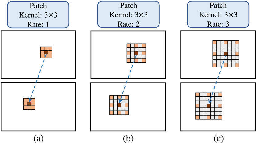
Attention weights generation. The attention weights aim to filter the initial concatenation volume so as to emphasize useful information and suppress irrelevant information. To this end, we generate attention weights by extracting geometric information from correlations between a pair of stereo images. Conventional correlation volume is obtained by computing pixel-to-pixel similarity which becomes unreliable for textureless regions due to lack of sufficient matching clues. To address this problem, we propose a more robust correlation volume construction method via multi-level adaptive patch matching (MAPM). Figure 3 illustrates the key idea of our MAPM. We obtain feature maps at three different levels $l_{1}$, $l_{2}$ and $l_{3}$ from the feature extraction module, and the number of channels for $l_{1}$, $l_{2}$ and $l_{3}$ is 64, 128 and 128 respectively. For each pixel at a particular level, we utilize an atrous patch with a predefined size and adaptively learned weights to calculate the matching cost. By controlling the dilation rate, we ensure that the patch’s scope is related to feature map level and meanwhile maintains the same number of pixels in similarity calculation for the center pixel. The similarity of two corresponding pixels is then a weighted sum of correlations between corresponding pixels within in the patch (denoted by red and orange colors in Figure 3).

We adopt the group-wise idea of GwcNet [7] to split features into groups and compute correlation maps group by group. Three levels feature maps of $l_{1}$, $l_{2}$ and $l_{3}$ are concatenated to form $N_{f}$-channel unary feature maps ($N_{f}$=320). We equally divide $N_{f}$ channels into $N_{g}$ groups ($N_{g}$=40), and accordingly the first 8 groups are from $l_{1}$, the middle 16 groups are from $l_{2}$, and the last 16 groups are from $l_{3}$. Feature maps of different levels will not interfere with each other. We denote the $gth$ feature group as $\mathbf{f}_{l}^{g}$, $\mathbf{f}_{r}^{g}$, and multi-level patch matching volume $\mathbf{C}_{patch}$ is computed as,

$$\begin{split}\mathbf{C}_{patch}^{l_{k}}(g,d,x,y)=\frac{1}{N_{f}/N_{g}}\sum\limits_{(i,j)\in\Omega^{k}}\omega_{ij}^{k,g}\cdot C_{ij}^{g}(d,x,y)\\ C_{ij}^{g}(d,x,y)=\langle\mathbf{f}_{l}^{g}(x\!-\!i,y\!-\!j),\mathbf{f}_{r}^{g}(x\!-\!i-\!d,y\!-\!j)\rangle,\end{split}$$

(2)

where $\mathbf{C}_{patch}^{l_{k}}$ ($k$$\in$$(1,2,3)$) represents matching cost of different feature level $k$. $\langle\cdot,\cdot\rangle$ is the inner product, $(x,y)$ represents the pixel’s location, and $d$ denotes different disparity level. $\Omega^{k}$=$(i,j)$ ($i,j$$\in$$(-k,0,k)$) is a nine-point coordinate set, defining the scope of the patch on the $k$-level feature maps (denoted by red and orange pixels in Figure 3 ($k$$\in$$(1,2,3)$). $\omega_{ij}^{k}$ represents the weight of a pixel $(i,j)$ in the patch on the $k$-level feature maps and is learned adaptively during the training process. The final multi-level patch matching volume is then obtained by concatenating matching costs $\mathbf{C}_{patch}^{l_{k}}$ ($k$$\in$$(1,2,3)$ of all levels,

$$\mathbf{C}_{patch}=\text{Concat}\left\{\mathbf{C}_{patch}^{l_{1}},\mathbf{C}_{patch}^{l_{2}},\mathbf{C}_{patch}^{l_{3}}\right\},$$

(3)

we denote the derived multi-level patch matching volume as $\mathbf{C}_{patch}\in\mathbb{R}^{N_{g}\times{D}/4\times{H}/4\times{W}/4}$, we then apply two 3D convolutions and a 3D hourglass network [7] to regularize $\mathbf{C}_{patch}$, and then use another convolution layer to compress the channels to 1 and derive the attention weights, i.e. $\mathbf{A}\in\mathbb{R}^{1\times{D}/4\times{H}/4\times{W}/4}$.

To obtain accurate attention weights of different disparity to filter the initial concatenation volume, we use ground truth disparity to supervise $\mathbf{A}$. Specifically, we adopt the same soft argmin function (in Equ. 5) as GC-Net [9] to obtain the disparity estimation $\mathbf{d}_{att}$ from $\mathbf{A}$. We compute smooth L1 loss between $\mathbf{d}_{att}$ and disparity ground truth to guide network learning process for deriving accurate attention weights $\mathbf{A}$.

Attention filtering. After obtaining the attention weights $\mathbf{A}$, we use it to eliminate redundant information in the initial concatenation volume and in turn enhance its representation ability. The attention concatenation volume $\mathbf{C}_{ACV}$ at channel $i$ is computed as,

$$\mathbf{C}_{ACV}(i)=\mathbf{A}\odot\mathbf{C}_{concat}(i),$$

(4)

where $\odot$ represents the element-wise product, and the attention weights $\mathbf{A}$ is applied to all channels of the initial concatenation volume.

Based on the ACV, we design an accurate and efficient end-to-end stereo matching network, named ACVNet. Figure 2 shows the architecture of our ACVNet which consists of four modules of unary feature extraction, attention concatenation volume construction, cost aggregation and disparity prediction. In the following, we introduce each module in details.

Feature extraction. We adopt the three-level ResNet-like architecture in  [7]. For the first three layers, three convolutions of $3{\times}3$ kernel with strides of 2, 1 and 1 are used to downsample the input images. Then, 16 residual layers [8] are followed to produce unary features at 1/4 resolution, i.e. $l_{1}$, 6 residual layers with more channels are followed to obtained large receptive fields and semantic information, i.e. $l_{2}$ and $l_{3}$. Finally, all feature maps ($l_{1}$, $l_{2}$, $l_{3}$) at 1/4 resolution are concatenated to form 320-channel feature maps for the generation of attention weights. Then two convolutions are applied to compress the 320-channel feature maps to 32-channel feature maps for construction of the initial concatenation volume, which are denoted as $\mathbf{f}_{l}$ and $\mathbf{f}_{r}$.

Attention concatenation volume construction. This module takes the 320-channels feature maps for attention weights generation, and $\mathbf{f}_{l}$ and $\mathbf{f}_{r}$ for initial concatenation volume construction. Then attention weights are used to filter the initial concatenation volume to produce a 4D cost volume for all disparities, as described in Section 3.1.

Cost aggregation. We process the ACV using a pre-hourglass module which consists of four 3D convolutions with batch normalization and ReLU, and two stacked 3D hourglass networks [7], each of which mainly consists of four 3D convolutions and two 3D deconvolutions stacked in an encoder-decoder architecture, see Figure 2.

Disparity prediction. Three outputs are obtained in the cost aggregation, see Figure 2. For each output, following GwcNet [7], two 3D convolutions are employed to output a 1-channel 4D volume, then we upsample and convert it into a probability volume by softmax function along the disparity dimension. Finally, the predicted value is computed by the soft argmin function [9],

$$d=\sum\limits_{k=0}^{D_{max}-1}k\cdot{p_{k}},$$

(5)

where $k$ denotes disparity level, $p_{k}$ denotes the corresponding probability. The three predicted disparity maps are denoted as $\mathbf{d}_{0}$, $\mathbf{d}_{1}$, $\mathbf{d}_{2}$.

We also construct a real-time version of ACVNet, named ACVNet-Fast. ACVNet-Fast adopts the same feature extraction but with fewer layers and disparity prediction modules as ACVNet. Figure 4 shows the architecture of ACVNet-Fast, the main differences between ACVNet-Fast and ACVNet lie in ACV construction and aggregation.

Specially, we construct the multi-level patch matching volume based on 1/8 resolution feature maps, and then use two 3D convolutions and a 3D hourglass network to regularize it to obtain the attention weights of 1/8 resolution i.e. $\mathbf{A}^{f}\in\mathbb{R}^{1\times{D}/8\times{H}/8\times{W}/8}$. To achieve real-time performance without sacrificing too much accuracy, we narrow disparity search space by sampling $h$($h$=6) hypotheses near the predicted disparity $\mathbf{d}_{att}^{f}\in\mathbb{R}^{H/2\times{W/2}}$ obtained by upsampled attention weights at 1/2 resolution. These hypotheses $\mathbf{D}_{hyp}\in\mathbb{R}^{h\times{H/2}\times{W/2}}$ is uniformly sampled within the range of $(\mathbf{d}_{att}^{f}-h/2,\mathbf{d}_{att}^{f}+h/2)$. According to these hypotheses, we construct sparse concatenation volume and sample attention weights to get sparse attention weights. Then we construct sparse attention concatenation volume $\mathbf{C}_{ACV}^{s}\in\mathbb{R}^{2N_{c}^{f}\times{6}\times{H}/2\times{W}/2}$ by Equ. 4.

For cost aggregation, we only use two 3D convolutions and one 3D hourglass network to regularize $\mathbf{C}_{ACV}^{s}$. As the matching information contained in $\mathbf{C}_{ACV}^{s}$ is very effective, only a very lightweight aggregation network is required. In this way, we achieve a good balance of accuracy and speed.

For ACVNet, the final loss is given by,

$$\begin{split}L=\lambda_{att}\cdot\text{Smooth}_{L_{1}}(\mathbf{{d}}_{att}-\mathbf{d}^{gt})+\\ \sum_{i=0}^{i=2}\lambda_{i}\cdot\text{Smooth}_{L_{1}}(\mathbf{d}_{i}-\mathbf{d}^{gt}),\end{split}$$

(6)

where $\mathbf{d}_{att}$ is obtained by attention weights $\mathbf{A}$ in Section 3.1. $\lambda_{att}$ represents the coefficient for the predicted $\mathbf{{d}}_{att}$, $\lambda_{i}$ represents the coefficient for the $ith$ predicted disparity and $\mathbf{d}^{gt}$ denotes the ground-truth disparity map. For ACVNet-Fast, the final loss is given by,

$$L^{f}=\lambda_{att}^{f}\cdot\text{Smooth}_{L_{1}}(\mathbf{{d}}_{att}^{f}-\mathbf{d}^{gt})+\lambda^{f}\cdot\text{Smooth}_{L_{1}}(\mathbf{{d}}^{f}-\mathbf{d}^{gt}),$$

(7)

where $\mathbf{d}^{f}$ is final output of ACVNet-Fast. The $\text{Smooth}_{L_{1}}$ is the smooth L1 loss.

Scene Flow is a collection of synthetic stereo datasets which provides 35454 training image pairs and 4370 testing image pairs with the resolution of 960$\times$540. This dataset provides dense disparity maps as ground truth. For Scene Flow dataset, we utilized the widely-used evaluation metrics end-point error (EPE) and percentage of disparity outliers D1. The outliers are defined as the pixels whose disparity errors are greater than $\text{max}(3\text{px},0.05d^{*})$, where $d^{*}$ denotes the ground-truth disparity.

KITTI includes KITTI 2012 [5] and KITTI 2015 [13]. KITTI 2012 and 2015 are datasets for real-world driving scenes. KITTI 2012 contains 194 training stereo image pairs and 195 testing images pairs, and KITTI 2015 contains 200 training stereo image pairs and 200 testing image pairs. Both datasets provide sparse ground-truth disparities obtained with LIDAR. The resolution of KITTI 2015 is 1242$\times$375, and that of KITTI 2012 is 1226$\times$370.

ETH3D is a collection of grayscale stereo pairs from indoor and outdoor scenes. It contains 27 training and 20 testing image pairs with sparse labeled ground-truth. Its disparity range is just in the range of 0-64. The percentage of pixels with errors larger than 2 pixels (bad 2.0) and 1 pixel (bad 1.0) are reported.

We implement our methods with PyTorch and perform our experiment using NVIDIA RTX 3090 GPUs. For all the experiments, we use the Adam [11] optimizer, with $\beta_{1}=0.9$, $\beta_{2}=0.999$. For ACVNet, the coefficients of four outputs are set as $\lambda_{att}$=0.5, $\lambda_{0}$=0.5, $\lambda_{1}$=0.7, $\lambda_{2}$=1.0. For ACVNet-Fast, the coefficients of two outputs are set as $\lambda_{att}^{f}$=0.5, $\lambda^{f}$=1.0. For Scene Flow, we first train attention weights generation network for 64 epochs and then train the remaining network for another 64 epochs. Finally we train complete network for 64 epochs. The initial learning rate is set to 0.001 decayed by a factor of 2 after epoch 20, 32, 40, 48 and 56. For KITTI, we finetune the pre-trained Scene Flow model on the mixed KITTI 2012 and KITTI 2015 training sets for 500 epochs. Then another 500 epochs are trained on the separate KITTI 2012/2015 training set. The initial learning rate is 0.001 and decreases by half at the 300th epoch.

Multi-level adaptive patch matching. The proposed multi-level adaptive patch matching is a general method that can be applied to most existing stereo models based on the correlation volume. In this study, we take GwcNet [7] as a baseline and replace the original point matching based correlation construction method with ordinary patch matching and our multi-level adaptive patch matching to derive three comparison methods, i.e., GwcNet [7], GwcNet-p and GwcNet-mp in Table 1. Ordinary patch matching utilizes a fixed size patch (3$\times$3) and equal weights for all pixels in the patch. Results show that only a slight improvement can be achieved by GwcNet-p compared with original GwcNet [7], but the proposed multi-level patch matching has a very significant improvement.

Attention concatenation volume. We evaluate different strategies for constructing the ACV on Scene Flow [12]. We still take GwcNet [7] as our baseline, replace its combined volume with our ACV and keep the subsequent aggregation and disparity prediction modules the same. Figure 5 shows three different ways of constructing the ACV. Figure 5 (a) directly averages the multi-level patch matching volume along the channel dimension and multiply it with the concatenation volume, denoted as GwcNet-mp-att. As shown in Table 1, just this simple approach can dramatically improve the accuracy. Apparently, when using multi-level patch matching volume to filter concatenation volume, the accuracy of multi-level patch matching volume is crucial and largely affects the final performance of the network, so we use an hourglass architecture of 3D convolutions to aggregate it, which is denoted as GwcNet-mp-att-hg shown in Figure 5 (b). The results in Table 1 show that GwcNet-mp-att-hg improve the D1 and EPE by 7.9% and 8.7% respectively compared with GwcNet-mp-att. To further explicitly constrain multi-level patch matching volume during training, we use the softmax and soft argmin function for regression to obtain the predicted disparity, and use the ground truth to supervise the disparity, denoted as GwcNet-mp-att-hg-s shown in Figure 5 (c). Compared with the GwcNet-mp-att-hg, GwcNet-mp-att-hg-s improves the D1 and EPE by 17.1% and 11.5% respectively with no computational cost increase in the inference stage. Overall, by replacing the combined volume in GwcNet [7] with our ACV, our GwcNet-mp-att-hg-s model achieves 42.8% and 39.5% improvement for D1 and EPE compared with GwcNet [7], demonstrating the effectiveness of ACV.

An ideal cost volume should require few parameters for subsequent aggregation network and meanwhile enable a satisfactory disparity prediction accuracy. In this subsection, we analyze the complexity of ACV in terms of the number of parameters demanded in the subsequent aggregation network and the corresponding accuracy. We use GwcNet [7] as the baseline. In original GwcNet [7], it uses a three stacked hourglass networks for cost aggregation. We first replace the combined volume in the original GwcNet [7] with our ACV with other parts remain the same. The corresponding model is denoted as Gwc-acv-3 in Table 2. The results show that compared with GwcNet [7], Gwc-acv-3 improves D1 and EPE by 42.8% and 39.5% respectively. We further reduce the number of hourglass networks from 3 to 2, 1, and 0, the correspondingly derived models are denoted as Gwc-acv-2, Gwc-acv-1 and Gwc-acv-0. The results in Table 2 show that, as the number of parameters reduced in the aggregation network, the prediction errors slightly increase. More importantly, after using our ACV, the stereo model without any hourglass network, i.e., Gwc-acv-0, even outperforms GwcNet. To achieve a both high accuracy and efficiency, we choose Gwc-acv-2 as our final model, and we denote it as ACVNet.

To demonstrate the universality of our ACV, we integrate our ACV into three state-of-the-art models, i.e. GwcNet [7], PSMNet [2] and CFNet [16], and compare the performance of the original models with those after using our ACV. Specifically, we denote the model after applying our method as GwcNet-ACV, PSMNet-ACV and CFNet-ACV for comparison respectively. As shown in Table 3, the EPE is reduced by 39.5% for GwcNet [7], 42.2% for PSMNet [2] and 14.4% for CFNet [16].

We experimentally compare our ACV with cascaded approaches. We apply the two-stage cascaded method proposed by  [6] to GwcNet, the corresponding model is denoted as Gwc-CAS. As shown in Table 4, our ACV outperforms cascaded approach. We think the superior performance of ACV to the cascaded approach is because the latter could suffer from irreversible cumulative errors as it directly discards disparities that is beyond the prediction range. However, our ACV only adjusts the weights of different disparities. Thus, although the attention weights are imperfect, the concatenation volume which contains rich context, can help amend errors to some extend via the subsequent aggregation network.

Scene Flow. As shown in Table 5, our method achieves state-of-the-art performance. We can observe that our ACVNet improves EPE accuracy by 38.4% and meanwhile has a faster inference speed compared with the state-of-the-art method LEAStereo[3], i.e. 0.2s vs. 0.3s.

KITTI. As shown in Table 7 and Figure 1, our ACVNet outperforms most existing published methods and ranks No.2 in KITTI 2012 and KITTI 2015 leaderboards. It is worth mentioning that our ACVNet is also the fastest among the top 10 methods in the KITTI benchmark leaderboards.

ETH3D. As shown in Table 5, our ACVNet outperforms the state-of-the-art methods, HITNet [18] and CFNet [16].

To sum up, our ACVNet shows excellent performance on the above four datasets, and it is worth mentioning that our ACVNet is also the only method that ranks top 5 concurrently in all four datasets, which represents the good generalization ability of our method to various scenes. The current SOTA methods always perform poorly in some certain scenarios, e.g. LEAStereo[3] has poor accuracy on Scene Flow; the performance of HITNet [18] in real-world scenarios (KITTI and ETH3D) is far inferior to our ACVNet.

To demonstrate the outstanding performance of our ACVNet-Fast, we compared it with the current classic real-time networks on Scene Flow [12] and KITTI [5, 13] benchmark. As shown in Table 6, our method achieves a very good balance between inference time and accuracy.

References

- [1] Rohan Chabra, Julian Straub, Christopher Sweeney, Richard Newcombe, and Henry Fuchs. Stereodrnet: Dilated residual stereonet. In Proceedings of the IEEE/CVF Conference on Computer Vision and Pattern Recognition, pages 11786–11795, 2019.
- [2] Jia-Ren Chang and Yong-Sheng Chen. Pyramid stereo matching network. In Proceedings of the IEEE Conference on Computer Vision and Pattern Recognition, pages 5410–5418, 2018.
- [3] Xuelian Cheng, Yiran Zhong, Mehrtash Harandi, Yuchao Dai, Xiaojun Chang, Tom Drummond, Hongdong Li, and Zongyuan Ge. Hierarchical neural architecture search for deep stereo matching. arXiv preprint arXiv:2010.13501, 2020.
- [4] Shivam Duggal, Shenlong Wang, Wei-Chiu Ma, Rui Hu, and Raquel Urtasun. Deeppruner: Learning efficient stereo matching via differentiable patchmatch. In Proceedings of the IEEE International Conference on Computer Vision, pages 4384–4393, 2019.
- [5] Andreas Geiger, Philip Lenz, and Raquel Urtasun. Are we ready for autonomous driving? the kitti vision benchmark suite. In 2012 IEEE conference on computer vision and pattern recognition, pages 3354–3361. IEEE, 2012.
- [6] Xiaodong Gu, Zhiwen Fan, Siyu Zhu, Zuozhuo Dai, Feitong Tan, and Ping Tan. Cascade cost volume for high-resolution multi-view stereo and stereo matching. In Proceedings of the IEEE/CVF Conference on Computer Vision and Pattern Recognition, pages 2495–2504, 2020.
- [7] Xiaoyang Guo, Kai Yang, Wukui Yang, Xiaogang Wang, and Hongsheng Li. Group-wise correlation stereo network. In Proceedings of the IEEE/CVF Conference on Computer Vision and Pattern Recognition, pages 3273–3282, 2019.
- [8] Kaiming He, Xiangyu Zhang, Shaoqing Ren, and Jian Sun. Deep residual learning for image recognition. In Proceedings of the IEEE/CVF Conference on Computer Vision and Pattern Recognition, pages 770–778, 2016.
- [9] Alex Kendall, Hayk Martirosyan, Saumitro Dasgupta, Peter Henry, Ryan Kennedy, Abraham Bachrach, and Adam Bry. End-to-end learning of geometry and context for deep stereo regression. In Proceedings of the IEEE International Conference on Computer Vision, pages 66–75, 2017.
- [10] Sameh Khamis, Sean Fanello, Christoph Rhemann, Adarsh Kowdle, Julien Valentin, and Shahram Izadi. Stereonet: Guided hierarchical refinement for edge-aware depth prediction. In European Conference on Computer Vision, 2018.
- [11] Diederik P Kingma and Jimmy Ba. Adam: A method for stochastic optimization. arXiv preprint arXiv:1412.6980, 2014.
- [12] Nikolaus Mayer, Eddy Ilg, Philip Hausser, Philipp Fischer, Daniel Cremers, Alexey Dosovitskiy, and Thomas Brox. A large dataset to train convolutional networks for disparity, optical flow, and scene flow estimation. In Proceedings of the IEEE Conference on Computer Vision and Pattern Recognition, pages 4040–4048, 2016.
- [13] Moritz Menze, Christian Heipke, and Andreas Geiger. Joint 3d estimation of vehicles and scene flow. ISPRS annals of the photogrammetry, remote sensing and spatial information sciences, 2:427, 2015.
- [14] Guang-Yu Nie, Ming-Ming Cheng, Yun Liu, Zhengfa Liang, Deng-Ping Fan, Yue Liu, and Yongtian Wang. Multi-level context ultra-aggregation for stereo matching. In Proceedings of the IEEE/CVF Conference on Computer Vision and Pattern Recognition, pages 3283–3291, 2019.
- [15] Thomas Schops, Johannes L Schonberger, Silvano Galliani, Torsten Sattler, Konrad Schindler, Marc Pollefeys, and Andreas Geiger. A multi-view stereo benchmark with high-resolution images and multi-camera videos. In Proceedings of the IEEE Conference on Computer Vision and Pattern Recognition, pages 3260–3269, 2017.
- [16] Zhelun Shen, Yuchao Dai, and Zhibo Rao. Cfnet: Cascade and fused cost volume for robust stereo matching. In Proceedings of the IEEE/CVF Conference on Computer Vision and Pattern Recognition, pages 13906–13915, 2021.
- [17] Xiao Song, Xu Zhao, Hanwen Hu, and Liangji Fang. Edgestereo: A context integrated residual pyramid network for stereo matching. In Asian Conference on Computer Vision, pages 20–35. Springer, 2018.
- [18] Vladimir Tankovich, Christian Hane, Yinda Zhang, Adarsh Kowdle, Sean Fanello, and Sofien Bouaziz. Hitnet: Hierarchical iterative tile refinement network for real-time stereo matching. In Proceedings of the IEEE/CVF Conference on Computer Vision and Pattern Recognition, pages 14362–14372, 2021.
- [19] Fangjinhua Wang, Silvano Galliani, Christoph Vogel, Pablo Speciale, and Marc Pollefeys. Patchmatchnet: Learned multi-view patchmatch stereo. In Proceedings of the IEEE/CVF Conference on Computer Vision and Pattern Recognition, pages 14194–14203, 2021.
- [20] Haofei Xu and Juyong Zhang. Aanet: Adaptive aggregation network for efficient stereo matching. In Proceedings of the IEEE/CVF Conference on Computer Vision and Pattern Recognition, pages 1959–1968, 2020.
- [21] Gengshan Yang, Joshua Manela, Michael Happold, and Deva Ramanan. Hierarchical deep stereo matching on high-resolution images. In Proceedings of the IEEE/CVF Conference on Computer Vision and Pattern Recognition, pages 5515–5524, 2019.
- [22] Chengtang Yao, Yunde Jia, Huijun Di, Pengxiang Li, and Yuwei Wu. A decomposition model for stereo matching. In Proceedings of the IEEE/CVF Conference on Computer Vision and Pattern Recognition, pages 6091–6100, 2021.
- [23] Jure Zbontar and Yann LeCun. Computing the stereo matching cost with a convolutional neural network. In Proceedings of the IEEE/CVF Conference on Computer Vision and Pattern Recognition, pages 1592–1599, 2015.
- [24] Feihu Zhang, Victor Prisacariu, Ruigang Yang, and Philip HS Torr. Ga-net: Guided aggregation net for end-to-end stereo matching. In Proceedings of the IEEE/CVF Conference on Computer Vision and Pattern Recognition, pages 185–194, 2019.
- [25] Youmin Zhang, Yimin Chen, Xiao Bai, Suihanjin Yu, Kun Yu, Zhiwei Li, and Kuiyuan Yang. Adaptive unimodal cost volume filtering for deep stereo matching. In Proceedings of the AAAI Conference on Artificial Intelligence, volume 34, pages 12926–12934, 2020.