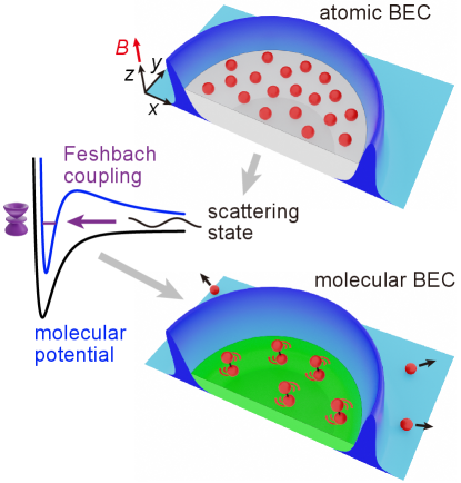
Atomic Bose-Einstein condensate to molecular Bose-Einstein condensate transition
Abstract
Preparation of molecular quantum gas promises novel applications including quantum control of chemical reactions, precision measurements, quantum simulation and quantum information processing. Experimental preparation of colder and denser molecular samples, however, is frequently hindered by fast inelastic collisions that heat and deplete the population. Here we report the formation of two-dimensional Bose-Einstein condensates (BECs) of spinning wave molecules by inducing pairing interactions in an atomic condensate. The trap geometry and the low temperature of the molecules help reducing inelastic loss to ensure thermal equilibrium. We determine the molecular scattering length to be Bohr and investigate the unpairing dynamics in the strong coupling regime. Our work confirms the long-sought transition between atomic and molecular condensates, the bosonic analog of the BEC-BCS (Bardeen-Cooper-Schieffer superfluid) crossover in a Fermi gas.
Because of their rich energy structure, cold molecules hold promises to advance quantum engineering and quantum chemistry Bohn2017 ; Carr2009 ; Quemener2012 ; a wide variety of platforms are developed to trap and cool cold molecules Carr2009 . The same rich energy structure, however, also causes complex reactive collisions that obstruct experimental attempts to cool molecules toward quantum degeneracy.
One successful strategy to prepare molecular quantum gas is to begin with an atomic quantum gas, and then pair the atoms into molecules Julienne2006 . A prominent example is the pairing of atoms in a two-component Fermi gas, which opens the door to exciting research on the BEC-BCS crossover Chen2005 ; Giorgini2008 . Recently, degenerate Fermi gas of ground state KRb molecules is observed based on quantum mixtures of Rb and K atoms Marco2019 . In these examples, molecules gain collisional stability from Fermi statistics and the preparation of molecules in the lowest rovibrational state, respectively.
For more generic molecules with many open inelastic channels, inelastic collision rates are difficult to predict and experiments frequently report rates near the unitarity limit, which means that all possible scatterings result in loss Mayle2013 ; Idziaszek2010 . The short lifetime hinders evaporative cooling toward quantum degeneracy.
Here we report the observation of BECs of Cs2 molecules in a high vibrational and rotational state, see Fig. 1. The molecules are produced by pairing Bose-condensed cesium atoms in a two-dimensional, flat-bottomed trap near a narrow wave Feshbach resonance Chin2010 . The trap geometry allows molecules to form with very low temperature and low collision loss such that the molecular condensates emerge in the Berezinskii-Kosterlitz-Thouless (BKT) superfluid regime Kruger2007 ; Tung2010 ; Hung2011nature ; Dalibard2011 . Our experiment opens exciting possibilities to investigate pairing and unpairing dynamics in a bosonic many-body system, described by the interaction Hamiltonian Romans2004 ; Leo2004 ; Timmermans2001 ; Duine2004
where and are the annihilation operators of a molecule and an atom, respectively, and is the coupling constant. Pairing in an atomic BEC is expected to induce a quantum phase transition into a molecular BEC Romans2004 .
Our experiment starts with a BEC of cesium atoms in a uniform optical trap. The radial confinement on the plane comes from a circular, flat-bottomed optical potential Clark2017 . The sample is vertically confined to a single site of an optical lattice with trap frequency Hz and radius 0.4 m. The atomic scattering length is at G, the global chemical potential is Hz and the temperature is nK, where is the Planck constant and is the Bohr radius.
We create Cs2 molecules by ramping the magnetic field across a closed-channel dominanted Feshbach resonance at G Herbig2003 . This resonance has a small width mG Innsbruck2018 and couples two scattering atoms into a weakly-bound molecule with a large orbital angular momentum and projection along the molecular axis . The molecules are short-ranged with the size given by the van der Waals length for Cs Chin2010 . This resonance is chosen due to the superior collisional stability between the molecules.
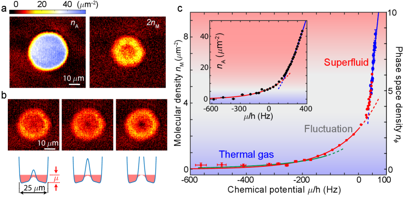
The ramp is optimized to pair up to of the atoms into molecules with the lowest achievable temperature Supplement . After the molecular formation, residual atoms are optically expelled from the trap and a magnetic field gradient is applied to levitate the molecules Herbig2003 . To detect the molecules, we dissociate them back to atoms by reversely ramping the field well above the resonance, and perform in situ imaging on the atoms, see Fig. 2a.
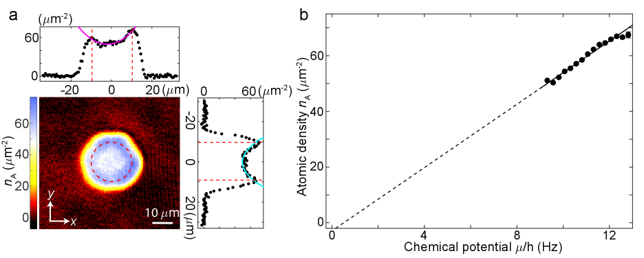
The produced molecules thus occupy the same trap volume as the atomic cloud. Slightly lower molecular density is observed at the trap center due to a weak magnetic field curvature of 21.5 on the plane. The field curvature leads to a slightly deeper potential in the rim than the center by nK for the molecules. The appearance of the ring structure in the molecular density profile, see Fig. 2a, suggests that the molecules are prepared at a temperature or chemical potential on the order of few nK.
To determine the molecular temperature, we find the conventional time-of-flight method impractical as the molecules expand very slowly within their lifetime. Instead we measure the density profile by slowly raising a potential barrier at the trap center over 10 ms and recording the density response, see Fig. 2b. With a high potential barrier, the molecules at the center becomes thermal with the density response , where is the Boltzmann constant. From fitting the data, we determine the molecular temperature to be 10(3) nK Supplement . The low temperature also suggests that the molecules form a 2D gas.
To probe the phase of the molecules at high densities, we measure the equation of state from their in situ density distribution Zhou2010 . Precise knowledge of the magnetic anti-trap potential is obtained from identical measurements with atomic condensates Supplement . The molecular density is found to linearly increase with the local chemical potential, consistent with the mean-field expectation , where is the 2D coupling constant Petrov2001 , is the 2D molecular density and is the molecular scattering length. Fitting the data with the theoretical prediction including finite temperature contribution Svistunov2002 ; Supplement , we obtain a temperature of nK, consistent with the optical barrier measurement.
We combine both measurements to determine the equation of state of the molecular gas. In Fig. 2c, we present the 2D density as a function of the local chemical potential . Notably, the transition from exponential to linear dependence on is the hallmark of the thermal gas to supefluid phase transition. A global fit to the data shows excellent agreement with the theory in the thermal and superfluid limits Supplement . From the fit, we determine the 2D coupling constant , molecular scattering length , the peak phase space density and the global chemical potential Hz. Repeated experiments in the range of show that is approximately constant. The peak phase space density exceeds the critical value for the BKT superfluid transition of (exp.)Hung2011nature and (theo.) Svistunov2001 at . In our flat-bottomed potential, we expect molecular condensation in the superfluid regime Dalibard2011 ; Supplement , and estimate to of the molecules are condensed.
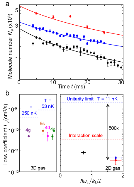
We further investigate the lifetime of the molecules. By holding the molecular BEC in the dipole trap with the initial mean density of , the sample survives for more than ms. Comparing samples with different densities and in different traps, we conclude that the decays are dominated by two-body collision loss Supplement , see Fig. 3a. The average loss coefficient of cm3/s for molecules in the 2D trap with Hz is significantly lower than previous measurements Ferlaino2010 ; Chin2005 , see Fig. 3b . It is also a factor of below the unitarity limit cms, where is the thermal average of the reciprocal molecular scattering wavenumber Idziaszek2010 ; Supplement , and a factor of below the interaction scale , see Fig. 3b.
The large suppression of inelastic collisions between the highly-excited wave molecules is remarkable. The comparison in Fig. 3b suggests that the collision loss is suppressed at low temperatures and possibly in the 2D regime Idziaszek2015 ; Micheli2010 . Since the unitarity limited loss scales as , smaller loss at lower temperature suggests that a larger suppression relative to the unitarity limit can be obtained by reaching down to even lower temperatures. At 10 nK, the loss coefficient we observe is already at the same level as the ground state fermionic molecules reported in Refs. Ye2011 ; Son2020 .
The observed lifetime of 30 ms is sufficient for many elastic collisions between molecules, which occur at the time scale of ms, to establish local thermal equilibrium. While the lifetime is insufficient to re-distribute molecules over the entire sample, thermal equilibrium in a (nearly) homogeneous system does not require global transport and can form by local interactions. It is remarkable that the measured temperatures at the trap center and in the rim are in good agreement with the atomic BEC at 11(2) nK. Our observation suggests that molecules are produced in thermal equilibrium with the atoms. As the result, the molecules are in thermal equilibrium with each other.
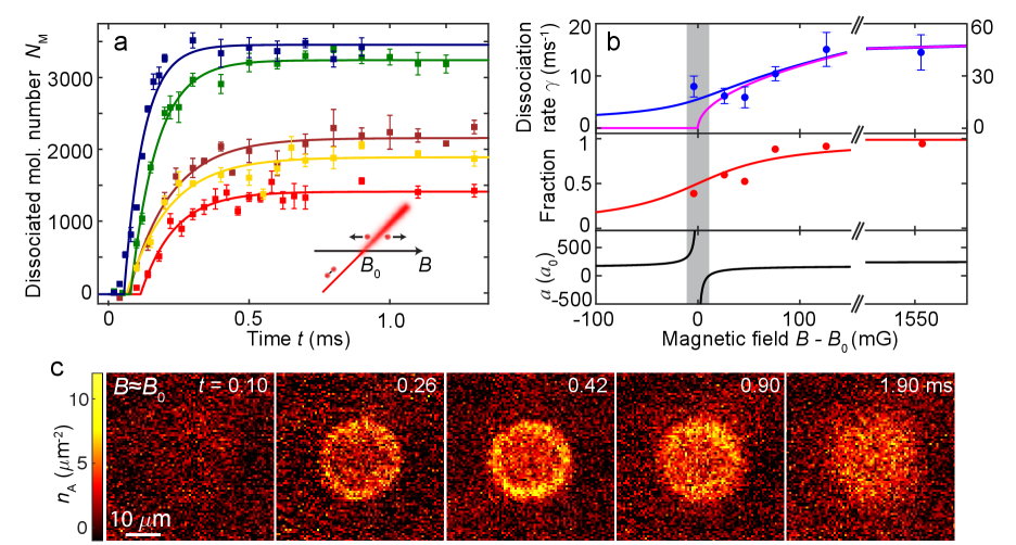
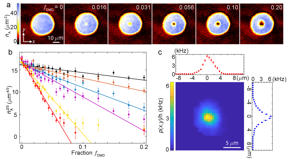
The molecular superfluid opens a new door to investigate pairing and unpairing in a Bose condensate. A phase transition is expected when unpairing occurs in a molecular BEC Romans2004 ; Leo2004 ; Timmermans2001 ; Duine2004 . Figure 4 presents our investigation into the unpairing dynamics. After forming the molecular condensate at G, we ramp the magnetic field in 0.3 ms near and above the Feshbach resonance with a precision of 2 mG. We monitor the dissociation process by imaging the emerging atoms.
When the field is ramped high above the resonance, the molecules quickly and entirely dissociate. In particular, the dissociation rate follows Fermi’s golden rule , where is the molecular energy above the continuum and kHz/G is the relative magnetic moment Chin2005 .
Near the Feshbach resonance the system enters the strong coupling regime and the measurement deviates from Fermi’s golden rule. Here the measured dissociation energy nK, see Fig. 4b, is much greater than and of the BEC and much smaller than the Feshbach resonance width . The energy is, however, comparable to the universal Fermi energy scale for the molecules . This result suggests that the dissociation dynamics near the Feshbach resonance is unitarity-limited Ho2004 ; Hadzibabic2018 . Finally, we observe about 40% of the molecules converted back to atoms, and attribute the missing 60% to inelastic collisions between atoms and molecules in the strong coupling regime.
To conclude, we realize BEC of high-excited, rotating molecules near a narrow Feshbach resonance. The molecules are sufficiently stable at low temperatures to ensure local thermal equilibrium. Unpairing dynamics in molecular condensates is consistent with the universality hypothesis. Our system offers a new platform to study the long-sought atomic BEC-molecular BEC transition, and highlights the fundamental difference between Cooper pairing in a degenerate Fermi gas and bosonic pairing in a BEC.
Acknowledgement
We thank P. Julienne for helpful discussions and K. Patel for carefully reading the manuscript. This work is supported by National Science Foundation (NSF) grant no. PHY-1511696, the Army Research Office Multidisciplinary Research Initiative under grant W911NF-14-1-0003 and the University of Chicago Materials Research Science and Engineering Center, which is funded by the NSF under grant no. DMR-1420709.
References
- (1) Bohn, J. L., Rey, A. M. & Ye, J. Cold molecules: Progress in quantum engineering of chemistry and quantum matter. Science 357, 1002–1010 (2017).
- (2) Carr, L. D., DeMille, D., Krems, R. V. & Ye, J. Cold and ultracold molecules: science, technology and applications. New Journal of Physics 11, 055049 (2009).
- (3) Quéméner, G. & Julienne, P. S. Ultracold molecules under control! Chemical Reviews 112, 4949–5011 (2012).
- (4) Köhler, T., Góral, K. & Julienne, P. S. Production of cold molecules via magnetically tunable Feshbach resonances. Rev. Mod. Phys. 78, 1311–1361 (2006).
- (5) Chen, Q., Stajic, J.,Tan, S. & Levin, K. BCS–BEC crossover: From high temperature superconductors to ultracold superfluids. Physics Reports 412, 1-88 (2005).
- (6) Giorgini, S., Pitaevskii, L.P., & Stringari, S. Theory of ultracold atomic Fermi gases. Rev. Mod. Phys. 80, 1215-1274 (2008).
- (7) De Marco, L. et al. A degenerate Fermi gas of polar molecules. Science 363, 853–856 (2019).
- (8) Mayle, M., Quéméner, G., Ruzic, B. P. & Bohn, J. L. Scattering of ultracold molecules in the highly resonant regime. Phys. Rev. A 87, 012709 (2013).
- (9) Idziaszek, Z., & Julienne, P. S. Universal rate constants for reactive collisions of ultracold molecules. Phys. Rev. Lett. 104, 113202 (2010).
- (10) Chin, C., Grimm, R., Julienne, P. & Tiesinga, E. Feshbach resonances in ultracold gases. Rev. Mod. Phys. 82, 1225–1286 (2010).
- (11) Krüger, P., Hadzibabic, Z. & Dalibard, J. Critical point of an interacting two-dimensional atomic Bose gas. Phys. Rev. Lett. 99, 040402 (2007).
- (12) Tung, S., Lamporesi, G., Lobser, D., Xia, L. & Cornell, E. A. Observation of the presuperfluid regime in a two-dimensional Bose gas. Phys. Rev. Lett. 105, 230408 (2010).
- (13) Hung, C.-L., Zhang, X., Gemelke, N. & Chin, C. Observation of scale invariance and universality in two-dimensional Bose gases. Nature 470, 236–239 (2011).
- (14) Hadzibabic, Z. & Dalibard, J. Two-dimensional Bose fluids: An atomic physics perspective. La Rivista del Nuovo Cimento 34, 389–434 (2011).
- (15) Romans, M. W. J., Duine, R. A., Sachdev, S. & Stoof, H. T. C. Quantum phase transition in an atomic Bose gas with a Feshbach resonance. Phys. Rev. Lett. 93, 020405 (2004).
- (16) Radzihovsky, L., Park, J. & Weichman, P. B. Superfluid transitions in bosonic atom-molecule mixtures near a Feshbach resonance. Phys. Rev. Lett. 92, 160402 (2004).
- (17) Timmermans, E., Furuya, K., Milonni, P. W. & Kerman, A. K. Prospect of creating a composite Fermi/Bose superfluid. Physics Letters A 285, 228–233 (2001).
- (18) Duine, R. A. & Stoof, H. T. C. Atom–molecule coherence in Bose gases. Physics Reports 396, 115–195 (2004).
- (19) Clark, L. W., Gaj, A., Feng, L. & Chin, C. Collective emission of matter-wave jets from driven Bose–Einstein condensates. Nature 551, 356–359 (2017).
- (20) Herbig, J. et al. Preparation of a pure molecular quantum gas. Science 301, 1510–1513 (2003).
- (21) Mark, M., Meinert, F., Lauber, K. & Nägerl, H.-C. Mott-insulator-aided detection of ultra-narrow Feshbach resonances. SciPost Phys 5, 055 (2018).
- (22) See supplementary materials.
- (23) Ho, T.-L. & Zhou, Q. Obtaining the phase diagram and thermodynamic quantities of bulk systems from the densities of trapped gases. Nature Physics 6, 131–134 (2010).
- (24) Petrov, D. S. & Shlyapnikov, G. V. Interatomic collisions in a tightly confined Bose gas. Phys. Rev. A 64, 012706 (2001).
- (25) Prokof’ev, N. & Svistunov, B. Two-dimensional weakly interacting Bose gas in the fluctuation region. Phys. Rev. A 66, 043608 (2002).
- (26) Prokof’ev, N., Ruebenacker, O. & Svistunov, B. Critical point of a weakly interacting two-dimensional Bose gas. Phys. Rev. Lett. 87, 270402 (2001).
- (27) Ferlaino, F. et al. Collisions of ultracold trapped cesium Feshbach molecules. Laser Physics 20, 23–31 (2010).
- (28) Chin, C. et al. Observation of Feshbach-like resonances in collisions between ultracold molecules. Phys. Rev. Lett. 94, 123201 (2005).
- (29) Idziaszek, Z., Jachymski, K. & Julienne, P. S. Reactive collisions in confined geometries. New Journal of Physics 17, 035007 (2015).
- (30) Micheli, A., Idziaszek, Z., Pupillo, G., Baranov, M. A., Zoller, P., & Julienne, P. S. Universal rates for reactive ultracold polar molecules in reduced dimensions. Phys. Rev. Lett. 105, 073202 (2010).
- (31) de Miranda, M. H. G. et al. Controlling the quantum stereodynamics of ultracold bimolecular reactions. Nature Physics 7, 502–507 (2011).
- (32) Son, H., Park, J. J., Ketterle, W. & Jamison, A. O. Collisional cooling of ultracold molecules. Nature 580, 197–200 (2020).
- (33) Ho, T.-L. Universal thermodynamics of degenerate quantum gases in the unitarity limit. Phys. Rev. Lett. 92, 090402 (2004).
- (34) Eigen, C. et al. Universal prethermal dynamics of Bose gases quenched to unitarity. Nature 563, 221–224 (2018).
- (35) Hung, C.-L. In situ probing of two-dimensional quantum gases (The University of Chicago, 2011).
- (36) Fano, U. Effects of configuration interaction on intensities and phase shifts. Phys. Rev. 124, 1866–1878 (1961).
Supplementary Material
I Experimental Procedure
The starting point of our experiment is a BEC of cesium atoms prepared in a disk-shaped dipole trap with a radius of 18 m in the horizontal plane. The disk-shaped potential is provided by a digital micromirror device (DMD) which projects 788 nm blue-detuned laser light on the plane with m resolution. The atoms are loaded into a single layer of the optical lattice in the vertical direction with trap frequency Hz CLthesis . A magnetic field gradient of 31 G/cm is applied to levitate the atoms and the magnetic field is tuned to 19.9 G.
We create the molecules with the wave narrow Feshbach resonance located at 19.87 G based on a procedure similar to Ref. Herbig2003 . Since atoms and molecules have different magnetic moments, they tend to separate vertically in the presence of a magnetic field gradient. To better confine both atoms and molecules in the molecular formation phase, we increase the magnetic field gradient to 42.5 G/cm in 2 ms before ramping the magnetic field to 19.76 G in 2 ms which creates molecules. After the formation of molecules, the magnetic field gradient is increased to 50 G/cm in 0.5 ms, which levitates the molecules and overlevitates the atoms.
To remove residual atoms after the molecular formation phase, a resonant light pulse of 20 s illuminates and pushes atoms away from the imaging area in 4 ms. Molecules are detected by reversely ramping the magnetic field which dissociates the molecules back to atoms, and the atoms are detected by absorption imaging. The final value of the magnetic field and the hold time are selected to give a reliable image that reflects the distribution of the molecules. In our experiments, we set the final magnetic field to be 20.44 G and do the detection in 0.1 ms after the reverse ramp. We estimate that the atoms expand by 1 m during the dissociation process, which is comparable with the imaging resolution of our experimental system.
II Characterization of external potential from atomic density profile
The strong magnetic field gradient for levitating the molecules leads to an additional magnetic anti-trapping potential on the horizontal plane. We also apply a central potential barrier projected from a DMD to measure the density response of the molecules. A precise knowledge of both the magnetic anti-trapping potential and the optical potential barrier are needed in order to extract the equation of state of the molecular gas.
We load atomic BEC into the same trap as for molecules to calibrate the external potential. Since the magnetic moment and polarizability of the g-wave molecule are accurately known, the trapping potential for molecules can thus be obtained from the trapping potential for atoms.
The magnetic anti-trap frequency in the horizontal plane is given by
| (S1) |
where , is magnetic moment, and are magnetic field and magnetic field gradient, respectively, at the location of particles and is determined from the coil geometry CLthesis . We determine the offset field value with an accuracy of 2 mG using microwave spectroscopy. We prepare atomic BEC at 17.2 G where the wave scattering length . Because of the low chemical potential, the atomic density distribution is sensitive to the magnetic anti-trap and shows lower density at the center and higher density in the rim, see Fig. S1a. Since the vertical trap frequency Hz is much larger than the chemical potential Hz, the BEC is in the quasi-2D regime and the column density under Thomas-Fermi approximation is given by
| (S2) |
where the 2D coupling strength , the magnetic anti-trap potential is parametrized by the trap frequencies and as and is the center position of the anti-trap. To determine the trap frequencies and the global chemical potential, we fit the in situ atomic density distribution using Eq. S2, see Fig. S1a. From the fit we get Hz, Hz and Hz. In this way, we calibrate the geometric parameters to be and , which we use to calculate the anti-trap frequencies for molecules based on Eq. S1, which gives Hz and Hz. For consistency check, we plot out the atomic density versus the local chemical potential , which agrees with the equation of state of a pure 2D BEC (see Fig. S1b).
We calibrate the optical potential barrier projected by DMD using atomic BEC prepared at 19.2 G, where the atomic scattering length is and the vertical trap frequency is Hz. The intensity of the optical barrier is ramped up within 10 ms. After waiting for another 2 ms, absorption imaging is performed in the vertical direction to record the atomic column density, see Fig. S2a. Here the barrier height is controlled by the fraction of micromirrors that are turned on. The fraction determines the intensity of the light projected onto the atom plane. In the region with higher light intensity, the atomic density is suppressed more, which in turn allows us to determine the light intensity. Because of the higher chemical potential of BEC in this case, the density depletion has a larger dynamical range that helps to calibrate larger range of barrier height. Since the chemical potential is comparable to the vertical trap frequency, the BEC is in 3D regime and the column density under Thomas-Fermi approximation is given by
| (S3) |
where , the 3D coupling strength and the local optical potential is proportional to the micromirror fraction as . Thus for each pixel located at (x,y), we have , from which the proportionality can be extracted from a series of measurements with different , see Fig. S2b. Repeating the same procedure for all the pixels within the region of optical barrier, we can map out the spatial dependence of the proportionality , see Fig. S2c. The polarizability of weakly bound molecules is approximately twice as large as that of a free atom, thus the corresponding proportionality for the molecules is .
After calibrating both the magnetic potential and the optical potential for molecules, we can get the local molecular density as a function of the total external potential and follow the fitting procedure in Sec. III to extract the global chemical potential . Then we obtain the corresponding local chemical potential and average the density in a certain spatial area with a proper range of local chemical potential to get the equation of state for molecules from the density profile and optical barrier measurements in Fig. 2. In addition, with the knowledge of the optical potential profile, we get the equation of state for the BEC in 3D regime, see the inset of Fig. 2c.
III Fitting the equation of state for 2D and 3D Bose gas
For a nondegenerate 2D ideal Bose gas, the phase space density is given by , where is the fugacity, and is the local chemical potential. If the gas is interacting, a mean field potential is added to the external potential based on the Hartree-Fock approximation Dalibard2011 . Then the equation of state for interacting 2D Bose gas becomes:
| (S4) |
which we use for fitting the data from the optical barrier measurement in Fig. 2c for density . On the other hand, the density of 2D superfluid outside the fluctuation region is Svistunov2001 :
| (S5) |
which we use for fitting the data from the density profile measurement in Fig. 2c for density .
We perform a global fit to the data points within the range and using Eq. S4 and Eq. S5, respectively, with temperature T, global chemical potential and 2D coupling constant as fitting parameters. Since the experimental condition drifted, the global chemical potential between the optical barrier and density profile measurements are different, and the chemical potential difference is also set as an free parameter in the global fit. The fit gives nK, and the global chemical potential for the optical barrier and density profile measurements as Hz and Hz, respectively. We also performed independent fits to the data at low density and high density . The resulting temperatures are nK and nK, in agreement with each other and with the global fit.
With the extracted 2D coupling constant , the critical phase density for BKT superfluid transition is evaluated as , where the coefficient Svistunov2001 . On the other hand, the BEC transition in our 2D box potential occurs at critical phase space density of Dalibard2011 , which coincides with the BKT transition.
IV Extraction of the two-body inelastic loss coefficients
In order to study the lifetime of g-wave molecules, we hold the molecules in different traps and monitor the decay of particle number as a function of the hold time. The two traps we used have horizontal radius , and vertical trap frequency Hz, Hz, respectively. The molecular density distribution in these traps are approximately uniform in the horizontal direction and Gaussian in the vertical direction, given by
| (S6) |
where = 1,2, and is the heaviside step function.
Even though the 1064 nm light intensity in the vertical direction of the two traps differ by a factor of , the decay rate of molecular number are similar, see Fig. 3a. This suggests that the one-body loss process due to the off-resonant laser light is negligible. In fact, since the g-wave molecules are in a highly excited rovibrational state, two-body loss process dominates which is modelled by . The molecular number decay corresponding to the density profile in Eq. S6 is thus given by
| (S7) |
where . We use Eq S7 to fit the data of molecular number decay and extract the inelastic loss coefficient in Fig. 3b.
The unitarity limit of the two-body loss coefficient is , where is the magnitude of the relative wavevector between two colliding molecules, associated with the relative kinetic energy Chin2010 . Due to the finite temperature in our experiment, the relative kinetic energy obeys Bolzmann distribution as , where the coefficient . The distrbution of the wavenumber is then given by
| (S8) |
The unitarity limit that we evaluate in Fig. 3b is , where the thermal average of with respect to the distribution is . For comparison with the loss coefficients, we evaluate the interaction scale as , where the 3D mean density .
V Empirical fit to dissociation rate and dissociated molecular fraction
After preparing a pure molecular BEC below the Feshbach resonance, if the magnetic field is then switched to a value high above the resonance, the molecules quickly dissociate into a continuum of free atoms. The dissociation rate follows Fermi’s golden rule as , where is the coupling matrix element between molecular and atomic states and is independent of the energy E above the continuum to leading order, the density of state and is the background scattering length. In this high field limit, our measured dissociation rate is consistent with Fermi’s golden rule , where the coefficient . The dissociation rate in Fig. 4b is extracted by fitting the data in Fig. 4a using the formula , where is the time when the molecules start to dissociate.
On the other hand, when the magnetic field is ramped to near the resonance where , we still observe a finite dissociation rate of . This is because the molecular state can couple to a band of scattering states that are Lorentzian distributed Fano1961 . We thus define an effective density of state to be a convolution between and a Lorentzian distribution. Thus the effective dissociation rate becomes
| (S9) |
where is the full width of the Lorentzian distribution. We use Eq. S9 to fit the dissociation rate as a function of the magnetic field we measured, shown as the blue solid line in the upper panel of Fig. 4b.
The dissociated molecular fraction drops when the magnetic field is ramped back closer to the resonance, which we attribute to the inelastic collision loss between atoms and molecules near the resonance. The data of the fraction in Fig. 4b is fitted using an empirical function , where and are set as free parameters.