AsynEIO: Asynchronous Monocular Event-Inertial Odometry Using Gaussian Process Regression
Abstract
Event cameras, when combined with inertial sensors, show significant potential for motion estimation in challenging scenarios, such as high-speed maneuvers and low-light environments. There are many methods for producing such estimations, but most boil down to a synchronous discrete-time fusion problem. However, the asynchronous nature of event cameras and their unique fusion mechanism with inertial sensors remain underexplored. In this paper, we introduce a monocular event-inertial odometry method called AsynEIO, designed to fuse asynchronous event and inertial data within a unified Gaussian Process (GP) regression framework. Our approach incorporates an event-driven frontend that tracks feature trajectories directly from raw event streams at a high temporal resolution. These tracked feature trajectories, along with various inertial factors, are integrated into the same GP regression framework to enable asynchronous fusion. With deriving analytical residual Jacobians and noise models, our method constructs a factor graph that is iteratively optimized and pruned using a sliding-window optimizer. Comparative assessments highlight the performance of different inertial fusion strategies, suggesting optimal choices for varying conditions. Experimental results on both public datasets and our own event-inertial sequences indicate that AsynEIO outperforms existing methods, especially in high-speed and low-illumination scenarios.
Index Terms:
event-inertial fusion, Gaussian process regression, motion estimation.I Introduction
The visual inertial odometry (VIO) technology is critical for autonomous robots to navigate in unknown environments. The VIO systems estimate motion states of robots by means of fusing Inertial Measurement Units (IMUs) and visual sensors. Generally, the Inertial Measurement Units (IMUs) directly measure angular velocities and linear accelerations while the visual sensors observe the bearing information with respect to environments. The complementarity of inertial and visual sensors makes the estimation problem more stable in both static and dynamic scenarios. Nevertheless, the conventional VIO systems are still prone to crash in several challenging scenarios, including high-speed movements, High-Dynamic-Range (HDR) environments, and sensors with incompatible frequencies. Specifically, high-speed movements and HDR environments will cause low-quality grayscale images for intensity cameras and long-period preintegration for IMUs. The long-period preintegration rapidly accumulates integration errors, meanwhile, low-quality images intend to deteriorate the visual frondend of VIO systems. Both of them result in a decline in estimation performance. In addition, discrete-time estimation and preintegration methods inherently have little support to fuse gyroscopes and accelerometers with incompatible frequencies or even asynchronous measurements. Therefore, it is imperative to develop a more robust VIO system to enhance estimation performance in challenging situations.
Event cameras have gained popularity in computer vision and robotics for applications such as object detection [1], image enhancement [2], and motion estimation [3, 4]. As a bio-inspired visual sensor, the event camera has an underlying asynchronous trigger mechanism where the illumination intensity variety of the scenario is independently recorded in a per-pixel manner. Benefiting from this special mechanism, event cameras gain prominent performance improvements to conventional cameras, such as low power consumption, low latency, HDR, high-temporal resolution, etc [5]. Intuitively, it means that event cameras has potential in motion estimation of high-speed and HDR scenarios. However, the discrete-time estimation framework adopted in event-based VIO systems greatly hinders the potential of event cameras as illustrated in [6].
Continuous-time estimation methods have been proposed to deal with foregoing drawbacks of event-based VIO systems. For these methods, a continuous-time trajectory is firstly defined with splines or kinematic assumptions, and then employed to build the measurement residuals. As the continuous-time trajectory have valid definitions at arbitrary timestamps, it naturally has the capacity of inferring the motion trajectory from totally asynchronous measurements and sensors. Among them, the Gaussian Process (GP) based methods have gained great interests of researchers for its clearer physical meaning. Although previous researchers have proposed to leverage GP-based methods to infer the SE(3) trajectory for event-based VIOs, existing methods still struggle to address the aforementioned challenges. With the introduction of GP-based methods, various inertial fusion schemes combining event cameras and IMUs have emerged. Thus, the interesting question is: which is the best fusion scheme for event-based VIO?
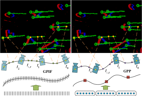
In this paper, we suggest an Asynchronous Event-Inertial Odometry (AsynEIO) system to improve the performance in challenging cases and comprehensively assess the reasonable inertial schemes. This study significantly builds on our previous conference publication [7] by developing a purely event-based frontend and introducing new inertial fusion schemes. The proposed AsynEIO utilizes a fully asynchronous fusion pipeline based on GP regression to improve the estimation performance in HDR and high-speed environments. Two main types of GP-based inertial fusion methods are integrated into the system to permit to fuse incompatible frequencies or asynchronous inertial measurements (i.e., GP-inertial Factor (GPIF) and GP-preintegration (GPP)), as depicted in Fig. 1. The GPIF is specifically designed for GP-based continuous-time methods to avoid the need for integrating raw measurements. We achieve this objective by leveraging a White Noise on Jerk (WNOJ) motion prior and investigating the underlying relationship between the differential SE(3) state variables and raw inertial measurements. Instead, the GPP infers data-driven GP models from real-time inertial measurements and generate a series of latent states to replace the motion prior in GPIF. Inspired by GPIF, we further extend the conventional discrete preintegration (Preint) to develop a new GP-based inertial factor, referred to as ExtPreint, where new residuals are directly incorporated into the GP trajectory. We fairly compare the performance of these inertial fusion methods under the unified event-inertial pipeline. Eventually, we conduct experiments on both public datasets and own-collected event-inertial sequences to demonstrate the advantages of the proposal with respect to the state-of-the-art. In summary, the main contributions of this article are as follows:
-
1.
A fully asynchronous event-inertial odometry named as AsynEIO that fuses pure event streams with inertial measurements using a unified GP regression framework.
-
2.
Comparative assessments of different inertial fusion schemes where four types of inertial schemes (i.e., GPIF, GPP, Preint, and ExtPreint) are compared to demonstrate the advantages of different fusion schemes.
-
3.
Comprehensive experiments conducted on both public datasets and own-collected sequences to show the improvements of our proposal with respect to the state-of-the-art.
The remainder of this paper is organized as follows. Sec. II reviews the relevant literature. The GP regression on with WNOJ are detailed in Sec. III. The GPP and GPIF are introduced in Sec. IV and Sec, V, respectively. The proposed AsynEIO with different inertial factors is described in Sec. VI. Experimental assessments are carried out in Sec. LABEL:sec:experiments. Finally, conclusions are drawn in Sec. VII.
II Related Work
Event-based visual-inertial odometry has gained significant research interest for challenging scenarios such as aggressive motion estimation as well as HDR scene. The most critical issue in this field is how to fuse data from the synchronous IMU data and the asynchronous event streams [5]. Zhu et al. [8] constructed a batch event packets aligning it by two Expectation-Maximization[9] steps and fused with pre-integration IMU in an EKF backend. Mahlknecht et al. [10] synchronized measurements from the EKLT tracker [11] using extrapolation when a fixed number of events is triggered. Then, these associated visual measurements was fused with IMU under a filter-based backend. However, the frontend computational complexity of these methods is very high. Rebecq et al. [12] detected corners on motion compensated event image and tracked through Lucas Kanade (LK) optical flow, and then fused the IMU-preintegrated measurements in a standard keyframe-based framework. Furthermore, this work was extended to the Ultimate-SLAM [4] by combing the standard frames. Lee et al. [13] proposed a 8-DOF warping model to fuse events and frames for accurate feature tracks. The residual from frontend optimization process was used to update an adaptive noise covariance. There is another trend of using the Time Surface (TS) [14] ,which stores the timestamp of the recent event at each pixel, as event representation to apply frame-based detection and tracking technique. [15] performed Arc* [16] for corner detection and LK tracking on TS with polarity. A tightly coupled graph-based optimization framework was designed to obtain estimation from the IMU and visual observations. PL-EVIO [17] combined the event-based line and point features and image-based point features to provide more information in human-made scene based on [15]. ESVO [18] proposed a first event-based stereo visual odometry by maximizing the spatio-temporal consistency using TS. Extended from [18], Junkai et al. [19] proposed a gyroscope measurements prior via pre-integration to circumvent the degeneracy issue. Kai et al. [20] utilized an adaptive decay-based TS to extract features and proposed a polarity-aware strategy to enhance the robustness, Then, these tracked features and IMU were fused in the MSCKF state estimator Overall, all these methods transform asynchronous event streams to synchronous data association and convert high rate IMU data into inter frame motion constrain through IMU-preintegration.
Another category of works directly processed event streams asynchronously [21, 16, 22, 23] and applied continuous-time state estimation methods to fuse asynchronous data. Unlike estimating discrete states, continuous-time estimation methods assume a continuous trajectory and approximates it through a set of basis functions. Interpolating on continuous trajectories, it can relate measurements observed at arbitrary times like multi cameras system [24], Lidar odometry [25, 26, 27] and event camera [28, 29]. Mueggler et al. [30] firstly used cubic B-splines trajectory representation to directly integrate the information tracked by a given line-based maps. Furthermore, to estimate the absolute scale, they fused pre-integration IMU between adjacent control points and extended [30] to point-based maps in [31]. Lu et al. [32] proposed event-based visual-inertial velometer which leveraged a B-spline continuous-time formulation to fuse the heterogeneous measurements from a stereo event camera and IMU. Besides the B-spline method, GP regression models the system’s motion state using GP and construct a GP prior between adjacent discrete states, like White-Noise-on-Acceleration (WNOA) prior [33] and WNOJ prior [34]. Wang et al. [28] applied a motion-compensated RANSAC and WNOA motion prior to a stereo event-based VO pipeline. Comparing the above two continuous trajectory representations, Johnson et al. [35] demonstrated the accuracy and computation time of WNOJ prior GP-based method and spline-based method are similar. Note that there is no work to implement the WNOJ prior to event-based odometry.
Recently, researchers have focused on designing new inertial fusion formulas specially for continuous-time estimation frameworks. Some of research works have proposed continuous-time formulations of IMU pre-integration [36, 37, 38]. These methods used inertial measurements to characterize the system’s continuous motion rather than direct prior like B-spline or GP-prior. [36] formulated a GP-based preintegration method for one-axis rotations and upsample the gyroscope data to compute the rotation preintegration when rotating on multiple axes. This strategy was employed in line features [39] and corner features [40] event-based VIO. IDOL [39] extracted event clusters of line segments and tracked lines between consecutive event windows. they leveraged [36] to associate asynchronous event measurements. However, this method shown a high computational cost for its full-batch optimization. Dai et al. [40] proposed a asynchronous tracking method relied on decaying event-based corners and adopted a similar fusing scheme as[39]. More recently, Gentil et al. [38] proposed a latent variable model to analytically integrate inertial measurements and implicitly induce a data-driven GP. This method formulated a unified GP-based integration to address the issue of continuous integration over SE(3) in [36]. Although their methods is specially designed for GP frameworks, they still integrate the inertial measurements rather than directly inferring on the raw measurements. Burnett et al. [41] introduced a velocity measurement model with integration in linear velocity under the WNOA motion prior [42]. Then, they further improve their methods with the Singer motion prior [27] where angular velocity and body-centric acceleration [43]. However, both of their methods accomplished poor preciseness in the accelerometer measurement model. Zheng et al. [25] developed a multi-LiDAR and IMU state estimator based on the GP-based trajectory. They separately defined the kinematic state on SO(3) and linear vector spaces rather than SE(3) and achieved a direct residual model on the raw measurements of IMUs. Chamorro et al. [44] investigated the event-IMU fusion strategies under Kalman filter which compared the conventional predict-with-IMU-correction-with-vision method and predict-with-model-correction-with-measurement. However, these solutions may face challenges in scenarios where straight lines are absent. Our previous work [7] investigated two different GP-based methods to fuse asynchronous visual measurements and IMU preintegration. Building on this foundation, we further extend our previous work to incorporate more inertial fusion methods and conduct comprehensive experiments to evaluate the performance of different schemes in fusing asynchronous measurements. In addition, our previous work relies on intensity images as auxiliary measurements for tracking event streams, limiting its performance in high-speed and HDR scenarios. In AsynEIO, we directly track pure event streams, achieving excellent adaptability in these challenging conditions.
III Sparse GP regression on
III-A Preliminaries and Kinematics
Define the transformation of the rigid body frame with respect to (w.r.t) the fixed inertial frame as a matrix , where the pose forms the special Euclidean group, denoted . Suppose the WNOJ prior to the kinematics of and apply the right multiply update of . We have the differential equation as follows:
| (1) | ||||
where
| (2) |
is the generalized velocity, is the generalized acceleration, and is the power spectral density matrix of the GP. Given the detailed rotation and translation components as
| (3) |
where maps the angular velocity vector to a skew-symmetric matrix. Then, we have . Comparing the subscripts, can be defined as , which represents the linear velocity of body frame w.r.t the inertial frame observed and expressed in the inertial frame. In fact, the generalized linear velocity indicates the same linear velocity observed in the inertial frame but expressed in the body frame. Notice that , where represents the linear velocity of body frame w.r.t the inertial frame observed and expressed in the body frame. Thereby, the generalized acceleration is given by
| (4) |
where . We know that and . Substituting them into (4), we can show
| (5) |
where represents the linear acceleration of body frame w.r.t the inertial frame observed and expressed in the inertial frame, and is the angular velocity of body frame w.r.t the inertial frame observed in the body frame. The kinematic state can be defined as
| (6) |
where the sub- and superscripts have been dropped and (III-A)-(5) describe the stochastic differential equations (SDEs) of kinematics. Since forms a manifold, these nonlinear SDEs are difficult to directly deploy in continuous-time estimation.
III-B GP Regression on Local Linear Space
To linearize it, the local variable in the tangent space of can be given by
| (7) |
where , and is the exponential map from to . The time derivative of (7) indicates the relationship between local variable and kinematic state as
| (8) |
where is the right Jacobian of . Notice that when is small enough. Further take the time derivative of (8), we can show the relationship between and :
| (9) |
Apply the first-order approximation and substitute (8), we have
| (10) |
where is the adjoint matrix operator. For our definition, we have
| (11) |
where is the rotation component and is the translation component. Now, we can define the local linear kinematic state w.r.t as
| (12) |
Similarly, we can assume the motion prior to be
| (13) |
On this basis, the linear time-invariant SDEs are
| (14) |
which has a closed-form solution for the state transition function . Meanwhile, the transition equation of the covariance matrix can be given by
| (15) |
III-C WNOJ Prior Residual
Under the WNOJ assumption, the GP prior residual between timestamp and can be defined as
| (16) |
in which , , , and . Notice that and are the inverse maps of and , respectively. We can compute the covariance matrix for prior residual from (15). Furthermore, the detailed Jacobians of prior residuals are listed in Appendix-C.
IV GP-Inertial Factor
The GPIF is directly built upon the continuous-time trajectory with the GP-based motion prior. The relationships between GP-based motion states and raw inertial measurements are derived as follows. Subsequently, the residuals and Jacobians are provided analytically.
IV-A Inertial Measurement Model
Generally, the measurement of the gyroscope is the noisy angular velocity , and the measurement of the accelerometer is the noisy value
| (17) |
where and are the Gaussian measurement noises, is the gravitational acceleration, and are biases that obey the Brownian movement.
| (18) | |||
| (19) |
where are covariance matrices.
IV-B GP-Inertial Residual and Jacobian
Before describing the GPIF, we need first know the kinematic state at an arbitrary timestamp. To query the trajectory at timestamp between and , we firstly interpolate the local variable with
| (20) |
Then, in conjunction with (7)-(12), the kinematic state in (6) can be resolved.
With the GP-based continuous-time trajectory, we construct the GPIF directly from the angular velocity and linear acceleration states, which avoids the preintegration. Considering (2), (5) and (17), the residual of GPIF can be given by
| (21) |
where the sub- and superscripts have been dropped. Neglecting the effects of bias and gravity, we can see that the raw acceleration measurement has a direct relationship with the kinematic state and an extra term . Notably, when the angular velocity or linear velocity is very small, or when the axis of rotation is approximately aligned with the direction of the linear velocity, this extra term can be neglected. In other cases, this extra term should be taken into account. Up to this point, we have established a detailed residual model between the raw IMU measurements and the kinematic states.
The covariance matrix of the direct residual is exactly the measurement covariance . The jacobians of GPIF residuals can be derived from the chain rule as follows:
| (22) |
where the derivations of can be found in the Appendix-D. Here, the nonzero components of are listed as follows:
| (23) |
where and are calculated with linear interpolation. In addition, a bias prior factor is attached between each pair of sampling timestamps and , as follows:
| (24) |
V GP-Preintegration
The GPP provides a different insight to utilize GP regression framework to tightly fuse inertial and other asynchronous measurements. Rather than conducting the kinematic prior, the GPP assumes local inertial measurements as a group of independent GPs and instantiates them on-the-fly in a data-driven manner.
V-A GP Assumptions on Local Measurements
Concretely, the GPP models the “local accelerations” and the “local angular velocities” as six independent GPs. Therefore, we have
| (25) | |||
where is the time derivative of , and are kernel functions of GPs, and is an identity matrix. The local variables are defined as
| (26) | ||||
in which is the rotation matrix of the body frame with respect to the inertial frame at the timestamp , and is so called the proper acceleration of the body frame. From the definition of (17), we know that . As shown in (25) and (26), the local accelerations and angular velocities are expressed in a local body frame at the timestamp . On this basis, these variables can be integrated linearly.
V-B GP-Preintegration on Induced Latent States
To permit efficient analytical preintegration, the GPP introduces a series of the latent states as the induced pseudo-observations and conducts an online optimization problem to infer them from inertial measurements. With the linear operator [45] defined on corresponding latent states, it can effectively execute the preintegration for given timestamps.
Suppose the latent states and be noisy observed vectors of local variables at the timestamp as in (25), we have
| (27) | ||||
where follows the zero-mean Gaussian distribution with a diagonal covariance matrix. By conditioning upon these latent states, the posterior values of local variables in (25) can be expressed as
| (28) | ||||
where is timestamp vector of desired latent states, is , is , is , and is . According to [38], the latent states can be recovered by means of constructing several optimization problems where the latent states and in (28) are optimized to predict a bunch of true IMU measurements as accurate as possible. After that, the preintegrated velocity , position and rotation vector increment can be written as:
| (29) | ||||
where is the queried timestamp. From (28), we know that the related variables of integration operations in (29) are only and . Indeed, the integration on latent states can be calculated analytically when and are given. The efficient analytical preintegration offers an ability for inferring on asynchronous measurements and continuous-time trajectories. The preintegration for the rotation matrix can be calculated with (26) as . Also, it is convenient to recover the kinematic state by means of composing the previous state with (29). With these composed states, the asynchronous visual projection can be done on arbitrary timestamps.
V-C Residual Terms for GP-Preintegration
VI Event-driven VIO
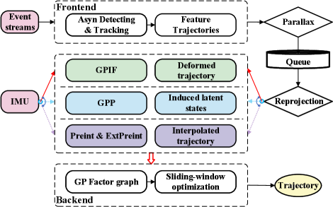
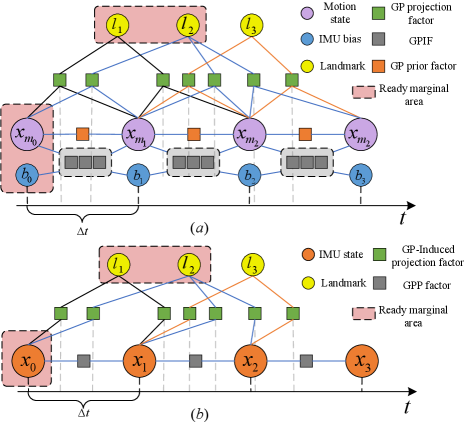
Given the GPIF and GPP , we design an event-inertial odometry that can estimate motion trajectory from pure event streams and inertial measurements. Both GPIF and GPP, in conjunction with the discrete preintegration [46], are built into the same EIO system (as shown in Fig. 2). This designment allows us to switch to different inertial fusion methods and compare them fairly.
VI-A Event-Driven Frontend
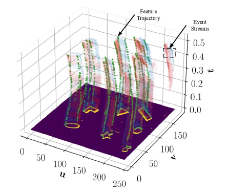
To realize high-temporal resolution, we design an asynchronous event-driven frontend where sparse features are detected and tracked in an event-by-event manner, as depicted in Fig. 3. Although separate event-driven feature detecting and tracking methods have been proposed in previous literature, a whole event-driven frontend needs further design on strategies of screening and maintenance. Concretely, we leverage a registration table to record the unique identifier of each active event feature. The pixel location of each event feature can be infer from its index in the registration table. Then, the unique identifier is mapped to the corresponding feature trajectory and its independent tracker. When a event measurement is obtained, we first search in the registration table to determine if its neighbor region already exists activate event features. If there is at least one active event feature, we utilize the identifier-tracker map to find the corresponding tracker and feed the event measurement to it. The movement of active feature will be reported by the tracker and collected into the feature trajectory. Otherwise, we update the SAE and determine if a FA-Harris [47] corner feature can be detected at the pixel location of this event measurement.
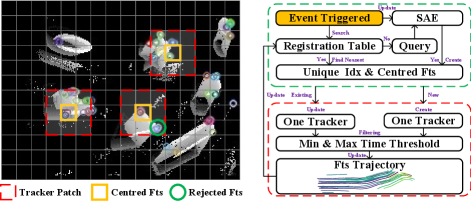
Since the registration table has the same width and height as the resolution of event cameras, it is high-efficient to access and modify elements in the registration table. The search of existing features only pays attention to a small patch within the registration table, and thus has a low time complexity. The small patch also reject the feature clustering and realize sparse features. Similarly, the detection only occurs at the location of the current event measurement and is thus efficient.
As the tracking of active features is triggered by subsequent events, a special case is that an active feature have not be triggered for a long time. For example, a corner feature is detected in noisy events by mistake, and thus it should be discarded promptly. To realize it, we assume the active feature should be triggered frequently within a maximum time threshold. We periodically delete the active features that have not been updated for more than the maximum time threshold. In addition, we also set a minimum time threshold to avoid the feature trajectory collecting a mass of redundant measurements. With patch search and time threshold mechanisms, the result frontend can obtain sparse and asynchronous feature tracking.
VI-B Asynchronous Repojection
The feature trajectory, uniquely indexed by , can be defined as
| (31) |
which represents an ordered spatial-temporal association set. The indicates the -th event feature measurement of the landmark at timestamp , and it contains
| (32) |
where is the measurement timestamp and is the observed pixel position.
When a feature trajectory has collected enough measurements for triangulation, the induced projection will be utilized to triangulate and embed these measurements into the underlying factor graph. Given the triangulated landmark and the event feature measurement as defined in (32), the projection model can be given by
| (33) |
where indicates the intrinsic matrix, is the depth of this landmark in current camera frame, is the extrinsic parameter of the event camera w.r.t the IMU, which can be solved by calibration. The kinematic state can be queried using (7) and (IV-B).
Different from the interpolated projection factor, the induced projection factor has reshaped the continuous-time trajectory using current accessible inertial measurements. Intuitively, it is more credible to build visual projection with this inertial induced factor. This concept is similar to the induce GP in the latent state preintegration method, while we leverage the proposed direct inertial factor to accomplish it. In contrast, the discrete preintegration scheme produces a unique pseudo-observation until the next sampling state. As a result, the asynchronous visual projection factors between inter-sampling states can only be interpolated under the motion prior assumption, which may sometimes lead to overly approximate results. Generally, both the direct factor and latent state preintegration can enhance the asynchronous projection of our event-driven VIO.
VI-C Inverse Depth Parametrization
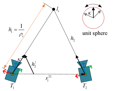
The inverse depth parametrization [48] is adopted to enhance the numerical stability and realize undelayed initialization. Different from the filter-based method in [48], we leverage this parametrization to optimize the GP-based factor graph and derive the analytical Jacobians. Furthermore, we define the directional vector in local frames rather than global frames, which is compatible with the optimization method. The (33) can be simplified as
| (34) |
We use the inverse depth , the directional vector in the unit sphere of the first camera pose observing this feature trajectory to represent the landmark . As displayed in Fig. 5, the latter camera pose should observe the ray and have a reprojected pixel location . When the poses and landmark are estimated precisely, this reprojected pixel location should coincide with the visual tracking result at the same camera pose. In fact, the direction of can uniquely determine the . From the geometric constraints in Fig. 5, the projected directional vector can be given by
| (35) |
where
| (36) |
Therefore, the projection function can be written as
| (37) |
where
| (38) |
It means the infinity landmark or the pure rotation when the inverse depth is for all time. In both situations, the pose and inverse depth can be optimized without ambiguity. Therefore, this parametrization permits immediate initialization of feature trajectories. The analytical Jacobians can be derived using the chain rule, as detailed in Appendix-E. Although inverse depth has a better numerical performance in optimization, it introduces more state variables (6-DoF first observed pose) in each projection factor. When the first observed pose occurs in inter-samples of the GP trajectory, it will increase further due to the GP interpolation (Two adjacent trajectory points with 36 dimensions). To alleviate this problem, we interpolate on the feature trajectory to find the closest sampling timestamp on the motion trajectory. The interpolated pixel position is then used to compute . This process initializes each feature trajectory for inverse depth optimization and reduces 30 dimensions for each projection factor. Benefited from high-time resolution of visual frontend, the interpolation on feature trajectories normally has negligible deviations.
VI-D Overall Cost Function in Sliding-Window
The primary advancement of GPIF is that it avoids the integral operations on raw measurements. For the micro-electro-mechanical systems (MEMS) IMU, these integral operations would introduce collective integral errors and deteriorate the estimation system after a fewer second. Instead, we establish the detailed relationship between the differential SE(3) states of the kinematic trajectory and the physical measurements obtained from the IMU. We find that the residual, Jacobians and covariance matrix for GPIF are elegant and suitable to be embedded into the GP-based factor graph. The overall cost for our event-driven VIO with GPIF is given by
| (39) |
where is the measurement covariance matrix of the event camera. We can see that there is only measurement covariance required by (VI-D) if the direct inertial factor is applied. Compared with preintegration schemes, we reduce the computational consumption paid for the covariance propagation. Also, this propagation is unreliable when the inertial measurements are partly lost or even asynchronous.
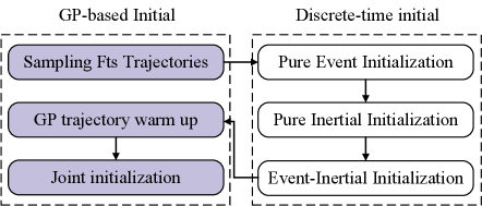
VI-E Event and Inertial Initialization
We design an initialization scheme (as shown in Fig. 7) to warm up our event-inertial system. The asynchronous continuous-time initialization is first converted to a synchronous discrete-time problem using a sampling strategy. A standard visual-inertial initialization method [49] is adopted to achieve initial estimating of pose, linear velocity and bias. With these known states, the remaining unknown states on the continuous-time GP trajectory are solved by a warm up optimization as
| (40) |
where and are the rotational velocity and generalized acceleration of the first trajectory point, and are two weight coefficients. This procedure adds some zero priors and limits the drift of GP trajectory in null space. Finally, a joint optimization as (VI-D) is built to add all asynchronous measurements and refine overall state variables.
VII Conclusion
This article introduces an asynchronous event-inertial odometry called AsynEIO that leverages a unified GP regression framework, where several important inertial fusion schemes are realized and evaluated. To the best of our knowledge, it is the first work that makes fair comparisons for asynchronous event-inertial fusion system. The expressing abilities of GP trajectories defined in different spaces and motion priors are assessed in detail, which can offer valuable suggest for choosing the suitable one according to certain conditions. The comparison analysis of various inertial factors explores their responses to sampling intervals and noises. We demonstrate that the GPP factor has greater contribution for inferring a fine-grained trajectory than GPIF and preintegration methods when the inertial measurements have low-level noises. Meanwhile, the GPP factor is more sensitive than other methods as the noise increases. Experiments conducted on real event-inertial sequences show that AsynEIO have a higher precision than the comparison method. Especially, our AsynEIO has a satisfied performance in high-speed maneuvering and low-illumination scenarios, which mainly benefited from the proposed asynchronous tracking and fusion mechanism. Although AsynEIO still need more improvements and engineering tricks for real-time estimation, we expect the proposed asynchronous event-inertial fusion framework and comparison results can contribute the community.
References
- [1] D. Gehrig and D. Scaramuzza, “Low-latency automotive vision with event cameras,” Nature, vol. 629, no. 8014, pp. 1034–1040, 2024.
- [2] G. Liang, K. Chen, H. Li, Y. Lu, and L. Wang, “Towards robust event-guided low-light image enhancement: A large-scale real-world event-image dataset and novel approach,” in Proc. IEEE/CVF Conf. Comput. Vis. Pattern Recognit., 2024, pp. 23–33.
- [3] Y.-F. Zuo, W. Xu, X. Wang, Y. Wang, and L. Kneip, “Cross-modal semi-dense 6-dof tracking of an event camera in challenging conditions,” IEEE Trans. Robot., vol. 40, pp. 1600–1616, 2024.
- [4] A. R. Vidal, H. Rebecq, T. Horstschaefer, and D. Scaramuzza, “Ultimate slam? combining events, images, and imu for robust visual slam in hdr and high-speed scenarios,” IEEE Robot. Autom. Lett., vol. 3, no. 2, pp. 994–1001, 2018.
- [5] G. Gallego, T. Delbrück, G. Orchard, C. Bartolozzi, B. Taba, A. Censi, S. Leutenegger, A. J. Davison, J. Conradt, K. Daniilidis et al., “Event-based vision: A survey,” IEEE Trans. Pattern Anal. Mach. Intell., vol. 44, no. 1, pp. 154–180, 2020.
- [6] Z. Wang, X. Li, T. Liu, Y. Zhang, and P. Huang, “Efficient continuous-time ego-motion estimation for asynchronous event-based data associations,” arXiv preprint arXiv:2402.16398, 2024.
- [7] X. Li, Z. Wang, Y. Zhang, F. Zhang, and P. Huang, “Asynchronous event-inertial odometry using a unified gaussian process regression framework,” in Proc. IEEE/RSJ Int. Conf. Intell. Robot. Syst. IEEE, 2024, accepted.
- [8] A. Zihao Zhu, N. Atanasov, and K. Daniilidis, “Event-based visual inertial odometry,” in Proc. IEEE/CVF Conf. Comput. Vis. Pattern Recognit., 2017, pp. 5391–5399.
- [9] A. Z. Zhu, N. Atanasov, and K. Daniilidis, “Event-based feature tracking with probabilistic data association,” in Proc. IEEE Int. Conf. Robot. Autom. IEEE, 2017, pp. 4465–4470.
- [10] F. Mahlknecht, D. Gehrig, J. Nash, F. M. Rockenbauer, B. Morrell, J. Delaune, and D. Scaramuzza, “Exploring event camera-based odometry for planetary robots,” IEEE Robot. Autom. Lett., vol. 7, no. 4, pp. 8651–8658, 2022.
- [11] D. Gehrig, H. Rebecq, G. Gallego, and D. Scaramuzza, “Eklt: Asynchronous photometric feature tracking using events and frames,” Int. J. Comput. Vis., vol. 128, no. 3, pp. 601–618, 2020.
- [12] H. Rebecq, T. Horstschaefer, and D. Scaramuzza, “Real-time visual-inertial odometry for event cameras using keyframe-based nonlinear optimization,” in Proc. British Mach. Vis. Conf., 2017.
- [13] M. S. Lee, J. H. Jung, Y. J. Kim, and C. G. Park, “Event-and frame-based visual-inertial odometry with adaptive filtering based on 8-dof warping uncertainty,” IEEE Robot. Autom. Lett., 2023.
- [14] X. Lagorce, G. Orchard, F. Galluppi, B. E. Shi, and R. B. Benosman, “Hots: a hierarchy of event-based time-surfaces for pattern recognition,” IEEE Trans. Pattern Anal. Mach. Intell., vol. 39, no. 7, pp. 1346–1359, 2016.
- [15] W. Guan and P. Lu, “Monocular event visual inertial odometry based on event-corner using sliding windows graph-based optimization,” in Proc. IEEE/RSJ Int. Conf. Intell. Robot. Syst. IEEE, 2022, pp. 2438–2445.
- [16] I. Alzugaray and M. Chli, “Asynchronous corner detection and tracking for event cameras in real time,” IEEE Robot. Autom. Lett., vol. 3, no. 4, pp. 3177–3184, 2018.
- [17] W. Guan, P. Chen, Y. Xie, and P. Lu, “Pl-evio: Robust monocular event-based visual inertial odometry with point and line features,” IEEE Trans. Autom. Sci. Eng., pp. 1–17, 2023.
- [18] Y. Zhou, G. Gallego, and S. Shen, “Event-based stereo visual odometry,” IEEE Trans. Robot., vol. 37, no. 5, pp. 1433–1450, 2021.
- [19] J. Niu, S. Zhong, and Y. Zhou, “Imu-aided event-based stereo visual odometry,” arXiv preprint arXiv:2405.04071, 2024.
- [20] K. Tang, X. Lang, Y. Ma, Y. Huang, L. Li, Y. Liu, and J. Lv, “Monocular event-inertial odometry with adaptive decay-based time surface and polarity-aware tracking,” arXiv preprint arXiv:2409.13971, 2024.
- [21] S. Hu, Y. Kim, H. Lim, A. J. Lee, and H. Myung, “ecdt: Event clustering for simultaneous feature detection and tracking,” in Proc. IEEE/RSJ Int. Conf. Intell. Robot. Syst. IEEE, 2022, pp. 3808–3815.
- [22] I. Alzugaray and M. Chli, “Haste: Multi-hypothesis asynchronous speeded-up tracking of events,” in Proc. Brit. Mach. Vis. Conf., 2020, p. 744.
- [23] X. Clady, S.-H. Ieng, and R. Benosman, “Asynchronous event-based corner detection and matching,” Neural Networks, vol. 66, pp. 91–106, 2015.
- [24] A. J. Yang, C. Cui, I. A. Bârsan, R. Urtasun, and S. Wang, “Asynchronous multi-view slam,” in Proc. IEEE Int. Conf. Robot. Autom. IEEE, 2021, pp. 5669–5676.
- [25] X. Zheng and J. Zhu, “Traj-lio: A resilient multi-lidar multi-imu state estimator through sparse gaussian process,” arXiv preprint arXiv:2402.09189, 2024.
- [26] P. Dellenbach, J.-E. Deschaud, B. Jacquet, and F. Goulette, “Ct-icp: Real-time elastic lidar odometry with loop closure,” in Proc. IEEE Int. Conf. Robot. Autom. IEEE, 2022, pp. 5580–5586.
- [27] J. N. Wong, D. J. Yoon, A. P. Schoellig, and T. D. Barfoot, “A data-driven motion prior for continuous-time trajectory estimation on se (3),” IEEE Robot. Autom. Lett., vol. 5, no. 2, pp. 1429–1436, 2020.
- [28] J. Wang and J. D. Gammell, “Event-based stereo visual odometry with native temporal resolution via continuous-time gaussian process regression,” IEEE Robot. Autom. Lett., vol. 8, no. 10, pp. 6707–6714, 2023.
- [29] D. Liu, A. Parra, Y. Latif, B. Chen, T.-J. Chin, and I. Reid, “Asynchronous optimisation for event-based visual odometry,” in Proc. IEEE Int. Conf. Robot. Autom., 2022, pp. 9432–9438.
- [30] E. Mueggler, G. Gallego, and D. Scaramuzza, “Continuous-time trajectory estimation for event-based vision sensors,” in Proc. Robot.: Sci. Syst., 2015.
- [31] E. Mueggler, G. Gallego, H. Rebecq, and D. Scaramuzza, “Continuous-time visual-inertial odometry for event cameras,” IEEE Trans. Robot., vol. 34, no. 6, pp. 1425–1440, 2018.
- [32] X. Lu, Y. Zhou, and S. Shen, “Event-based visual inertial velometer,” arXiv preprint arXiv:2311.18189, 2023.
- [33] T. D. Barfoot, C. H. Tong, and S. Särkkä, “Batch continuous-time trajectory estimation as exactly sparse gaussian process regression.” in Proc. Robot.: Sci. and Syst., vol. 10. Citeseer, 2014, pp. 1–10.
- [34] T. Y. Tang, D. J. Yoon, and T. D. Barfoot, “A white-noise-on-jerk motion prior for continuous-time trajectory estimation on se(3),” IEEE Robot. Autom. Lett., vol. 4, no. 2, pp. 594–601, 2019.
- [35] J. Johnson, J. Mangelson, T. Barfoot, and R. Beard, “Continuous-time trajectory estimation: A comparative study between gaussian process and spline-based approaches,” arXiv preprint arXiv:2402.00399, 2024.
- [36] C. Le Gentil, T. Vidal-Calleja, and S. Huang, “Gaussian process preintegration for inertial-aided state estimation,” IEEE Robot. Autom. Lett., vol. 5, no. 2, pp. 2108–2114, 2020.
- [37] C. Le Gentil and T. Vidal-Calleja, “Continuous integration over so (3) for imu preintegration,” Robot.: Sci. Syst., 2021.
- [38] ——, “Continuous latent state preintegration for inertial-aided systems,” Int. J. Robot. Res., vol. 42, no. 10, pp. 874–900, 2023.
- [39] C. Le Gentil, F. Tschopp, I. Alzugaray, T. Vidal-Calleja, R. Siegwart, and J. Nieto, “Idol: A framework for imu-dvs odometry using lines,” in Proc. IEEE/RSJ Int. Conf. Intell. Robot. Syst. IEEE, 2020, pp. 5863–5870.
- [40] B. Dai, C. Le Gentil, and T. Vidal-Calleja, “A tightly-coupled event-inertial odometry using exponential decay and linear preintegrated measurements,” in Proc. IEEE/RSJ Int. Conf. Intell. Robot. Syst. IEEE, 2022, pp. 9475–9482.
- [41] K. Burnett, A. P. Schoellig, and T. D. Barfoot, “Continuous-time radar-inertial and lidar-inertial odometry using a gaussian process motion prior,” arXiv preprint arXiv:2402.06174, 2024.
- [42] S. Anderson and T. D. Barfoot, “Full steam ahead: Exactly sparse gaussian process regression for batch continuous-time trajectory estimation on se (3),” in Proc. IEEE/RSJ Int. Conf. Intell. Robot. Syst. IEEE, 2015, pp. 157–164.
- [43] K. Burnett, A. P. Schoellig, and T. D. Barfoot, “Imu as an input vs. a measurement of the state in inertial-aided state estimation,” arXiv preprint arXiv:2403.05968, 2024.
- [44] W. Chamorro, J. Solà, and J. Andrade-Cetto, “Event-imu fusion strategies for faster-than-imu estimation throughput,” in Proc. IEEE/CVF Conf. Comput. Vis. Pattern Recognit., 2023, pp. 3975–3982.
- [45] S. Särkkä, “Linear operators and stochastic partial differential equations in gaussian process regression,” in Artificial Neural Networks and Machine Learning – ICANN 2011. Springer, 2011, pp. 151–158.
- [46] C. Forster, L. Carlone, F. Dellaert, and D. Scaramuzza, “On-manifold preintegration for real-time visual–inertial odometry,” IEEE Trans. Robot., vol. 33, no. 1, pp. 1–21, 2016.
- [47] R. Li, D. Shi, Y. Zhang, K. Li, and R. Li, “Fa-harris: A fast and asynchronous corner detector for event cameras,” in Proc. IEEE/RSJ Int. Conf. Intell. Robot. Syst. IEEE, 2019, pp. 6223–6229.
- [48] J. Civera, A. J. Davison, and J. M. Montiel, “Inverse depth parametrization for monocular slam,” IEEE Trans. Robot., vol. 24, no. 5, pp. 932–945, 2008.
- [49] T. Qin, P. Li, and S. Shen, “Vins-mono: A robust and versatile monocular visual-inertial state estimator,” IEEE Trans. Robot., vol. 34, no. 4, pp. 1004–1020, 2018.
Appendix
VII-A Adjoint of
| (41) |
where , is the right Jacobian matrix.
| (42) |
VII-B Perturbing the Pose on
| (43) | ||||
| (44) |
VII-C Perturbing WNOJ Prior Residuals
| (45) |
| (46) |
| (47) | ||||
| (48) | ||||
| (49) | ||||
| (50) |
| (51) |
| (52) |
| (53) |
VII-D Jacobians of Interpolated State w.r.t Sampling States
The relationship between the linear local state and kinematic state at sampling timestamps is
| (54) | ||||
| (55) |
The interpolated local state can be expressed with sampling states as
| (56) | ||||
| (57) | ||||
| (58) |
Notice that and have the same forms as , but have different rows of matrix coefficients. With (8) and (9), we can resolve and .
We first derive the perturbing Jacobians of w.r.t and , respectively. Then, the perturbing Jacobians of w.r.t and are given.
| (59) |
| (60) |
| (61) |
According the chain rule, we can define the Jacobians of interpolated state w.r.t and as
| (62) | ||||
| (63) |
Perturbing the right-hand side of (8) with and , we have
| (64) | ||||
| (65) | ||||
| (66) | ||||
| (67) |
On this basis, the Jacobians of w.r.t the local variables are given by
| (68) | ||||
| (69) | ||||
| (70) |
Calculating the derivative on both sides of (8) yields
| (71) |
Therefore, we have the Jacobians as
| (72) | ||||
| (73) | ||||
| (74) |
Perturbing the right-hand side of (56) with , and , we have
| (75) |
Therefore, we have Jacobians as follows:
| (76) | ||||
| (77) | ||||
| (78) | ||||
| (79) | ||||
| (80) | ||||
| (81) |
VII-E Jacobians of Visual Residuals
| (82) | ||||
| (83) |
| (84) | ||||
| (85) |
| (86) |
| (87) | ||||
| (88) | ||||
| (89) |
| (90) |
| (91) | ||||
| (92) |