Asynchronous Blob Tracker for Event Cameras
Abstract
Event-based cameras are popular for tracking fast-moving objects due to their high temporal resolution, low latency, and high dynamic range. In this paper, we propose a novel algorithm for tracking event blobs using raw events asynchronously in real time. We introduce the concept of an event blob as a spatio-temporal likelihood of event occurrence where the conditional spatial likelihood is blob-like. Many real-world objects such as car headlights or any quickly moving foreground objects generate event blob data. The proposed algorithm uses a nearest neighbour classifier with a dynamic threshold criteria for data association coupled with an extended Kalman filter to track the event blob state. Our algorithm achieves highly accurate blob tracking, velocity estimation, and shape estimation even under challenging lighting conditions and high-speed motions ( 11000 pixels/s). The microsecond time resolution achieved means that the filter output can be used to derive secondary information such as time-to-contact or range estimation, that will enable applications to real-world problems such as collision avoidance in autonomous driving. Project Page: https://github.com/ziweiwwang/AEB-Tracker
Index Terms:
Event-based Camera, Event Blob, High-Speed Target Tracking, Asynchronous Filtering, Real-time Processing, Time to Contact, Range Estimation, High Dynamic Range.I Introduction
 |
Object tracking is a core capability in a wide-range of robotics and computer vision applications such as simultaneous localisation and mapping (SLAM), visual odometry (VO), obstacle avoidance, collision avoidance, autonomous driving, virtual reality, smart cities, etc [1]. Real-time visual tracking of high-speed targets in complex environments and in low light poses significant challenges due to their fast movement and complex visual backgrounds. Traditional frame-based tracking methods are often hardware-limited as images are susceptible to motion blur, low frame rates and low dynamic range. Event cameras offer significant advantages in these scenarios. Instead of accumulating brightness within a fixed frame rate for all pixels, event cameras capture only changing brightness at a pixel-by-pixel level. Quickly moving foreground objects generate more events than complex visual backgrounds making the event camera sensor modality ideal for high-performance real-world target tracking.
In this paper, we propose an asynchronous event blob tracker (AEB tracker) for event cameras. The targets considered are modelled as a spatio-temporal event likelihood where the conditional spatial likelihood is blob-like, a structure we term an event blob [2]. A key advantage is that the event blob concept fundamentally includes the temporal aspect of event data. In particular, we use a spatial Gaussian likelihood with time-varying mean and covariance to model the unipolar event blob (where both polarities are equally considered). The state considered includes position (mean of the event blob), non-homogeneous spatial cross-correlation of the event blob (encoded as two principal correlations and an orientation), and both the linear and angular velocity of the blob. In the case of a non-flickering blob an additional polarity offset shape parameter is used as well. Our AEB tracker uses an extended Kalman filter that accepts raw event data and uses each event directly to update a stochastic state-estimate asynchronously. A key novelty of the algorithm is that the filter states for the shape of the distribution are used as stochastic parameters in the generative measurement model. This formulation is non-standard in classical extended Kalman filters. To do this we construct two pseudo measurement functions based on normalised position error and chi-squared variance. These pseudo measurements provide information about the spatial variance of the event blob and ensure observability of the shape parameters of the target. The proposed model enables adaptive estimation of blob shape allowing our AEB tracker to function effectively across a wide range of motion and shape tracking problems. In particular, adaptive shape estimation allows our algorithm to operate without dependence on scenario-specific prior knowledge.
The asynchronous filter state is updated after each event (associated with a given blob), coupling the filter update rate to the raw event rate of the blob tracked. For scenarios with low background noise, the foreground event rate is limited only by the microsecond physical limits of the camera (data bus, circuit noise and refractory period limitations of the camera etc [3]) and, even in poor lighting conditions, filter updates in excess of 50kHz are possible.
We evaluate the proposed algorithm on two indoor experiments, with extremely fast target speeds and camera motions; and two outdoor real-world case studies, including tracking automotive tail lights at night and tracking a quickly moving aerial vehicle. In the first indoor experiment, we track a spinning blob with controllable speeds, ranging from low to very high optical flow (greater than 11000 pixels/s), and compare the proposed algorithm to the most relevant state-of-the-art event-based tracking algorithms. In the second indoor experiment, we shake the camera in an unstructured pattern to demonstrate the tracking performance under rapid changes of direction of the image blobs. In our first outdoor real-world case study, we track multiple automotive tail lights in a night driving scenario. Due to the high event rates induced by the flickering LED lights, the filter achieves update rates of over 100kHz with high signal-to-noise ratio. The quality of the filter data is validated by computing robust, high-bandwidth, time-to-contact estimates from the visual divergence between tail lights on a target vehicle. In the second outdoor real-world case study, we track and estimate the event distribution of a high-speed aerobatic quadrotor in difficult visual conditions and in front of complex visual backgrounds. The visual shape estimation of the target event blob is used to infer range information demonstrating the utility of the shape parameter estimation and quality of the filter estimate.
The primary contributions of the paper are:
-
•
A novel asynchronous event blob tracker for real-time high-frequency event blob tracking.
-
•
A novel modification of extended Kalman filter theory to estimate shape parameters of event blob targets.
-
•
Demonstration of the performance of the proposed algorithm on two experimental and two real-world case studies with challenging datasets.
The datasets and source code are provided open-source for future comparisons.
II Related Works
The first high-speed, low-latency tracking algorithm for dynamic vision sensors was developed in 2006 [4]. Its application in the robotic goalie task was studied in subsequent works [5, 6]. Recently, event cameras have been used in a range of blob-like object tracking applications including star tracking [7, 8, 9]; high-speed particle tracking [10, 11, 12]; and real-time eye tracking [13, 14]. The tracking algorithms developed for these applications have, in the most part, been bespoke algorithms that exploit specific target, motion or background properties and have a limited ability to generalise to other scenarios.
General-purpose event-based tracking algorithms have focused on corner and template tracking. The corner tracking algorithms can be categorised into window-based data association or clustering methods [15, 16, 17, 18], asynchronous event-only methods [19, 20, 21, 22, 23, 24], and asynchronous methods that use hybrid event-frame data [25, 24]. Template-based methods for event cameras tend to be highly dependent on the scenario. Mueggler et al. [26] used a stereo event camera to detect and track spherical objects for collision avoidance. Mitrokhin et al. [27] estimated relative camera motion from a spatio-temporal event surface, then segmented and tracked moving objects based on the mismatch of the local event surface. Falanga et al. [28, 29] demonstrated the importance of low latency for sense-and-avoid scenarios. Their experiments used 10ms windowed event data and classical blob tracking algorithms. Sanket et al. [30] developed an onboard neural network for the same sense-and-avoid scenario. Rodriguez-Gomez et al. [31] used asynchronous corner tracking and then clustered corners to create objects that are tracked. Li et al. [32] and Chen et al. [33] converted event streams into pseudo-frames and then tracked objects using frames. Recent work has seen considerable effort in deep learning methods for object tracking [34, 35, 30, 36, 37, 38]. A disadvantage of such methods is that they require a large amount of training data. In addition, Convolutional Neural Network (CNN) algorithms rely on data windowing to create pseudo-frames, compromising low-latency and real-time performance [35, 38]. Other state-of-the-art networks, such as Spiking Neural Network (SNN) and Graph Neural Network (GNN) [36, 37], although promising in various aspects, are intractable to run in real-time at kHz rates due to their large scale and computational complexity.
The combination of conventional frames and event cameras has also been explored for object tracking [39, 40], enabling the use of data association techniques derived from classical computer vision literature. Active LED lights are commonly used to create event blob targets for experimental work. Müller et al. [41] used LED markers in a low-power embedded Dynamic Vision Sensor system and introduced two active LED marker tracking algorithms based on event counting and the time interval between events. Censi et al. [42] mounted LED markers on a flying robot and proposed a low-latency tracking method that associated LED markers based on the time interval between events and then tracked each LED light using a particle filter. Wang et al. [43] used active LED lights for high-speed visual communication with conventional blob detection and tracking methods on pseudo-frames. These LED tracking methods usually require the targets to blink in known or very high frequencies. A characteristic of the schemes discussed is that data association is mostly built into an asynchronous pre-processing module, such as a corner detector, clustering algorithm or frame-based correlation; or the algorithm requires pseudo-frames, event-frames or estimation of an event surface over a window of data. Such architectures lead to increased latency and reduced frequency response of target tracking, although many of the algorithms reviewed still achieve excellent results, especially when compared to classical frame-based image tracking.
III Problem Formulation
In this section we formulate the problem of tracking event blob targets.
III-A Spatio-Temporal Gaussian Likelihood Model for Event Blob Targets
Event cameras report the relative log intensity change of brightness for each pixel asynchronously. We consider the likelihood of an event occurring at pixel location at time and with polarity . We will term such a likelihood model an event blob if the spatial distribution of the conditional likelihood for a fixed time is blob-like. We propose a spatio-temporal Gaussian event blob likelihood function
| (1) | ||||
where is the pixel location of the centre of the object and is the shape of the object (encoded as the principal square root of the second-order moment of the event spatio-temporal intensity). The positive-definite matrix is written
| (2) |
for principal correlations and orientation angle where is the associated rotation matrix. The scalar encodes the temporal dependence of the likelihood associated with changing event rate and denotes a binomial distribution associated with whether the event has polarity depending on position and time. If is integrable on a time interval of interest, then the spatio-temporal Gaussian event blob likelihood could be normalised to produce a probability density on this time interval. In this paper, however, we will use the conditional likelihood , a spatial Gaussian distribution with time-varying parameters. In the sequel, we will often omit the time index from the state variables , , etc., to make the notation more concise.
The archetypal examples of event blob targets are flickering objects such as an LED or fluorescent light [44]. A flickering target generates events at pixel locations in proportion to the frequency of the flicker and intensity of the source at that pixel. The likelihood of an event occurring at a given moment in time is proportional to the rate of events and the binomial probability of polarity is independent of position. Thus, for a target with constant flicker, the spatial distribution of the unipolar (ignoring event polarity) event blob likelihood is directly related to the intensity of the source and is analogous to image intensity. An example of the event arrival histogram for LED tail lights of cars is shown in the top row of Figure 2. Here the image blobs in Figure 2b-c are roughly Gaussian.
 |
In the case of a non-flickering target, the situation is more complex since the motion of the target in the image plane is required to generate events. In this case, the events are asymmetrically arranged around the target centre depending on whether the target is bright or dark with respect to the background and the binomial distribution is not independent of the spatial parameter . For a bright target against a dark background, the events in the direction of motion are positive while the trailing events are negative, and vice-versa if the background is brighter than the target. If both positive and negative events are equally considered, then the resulting density is symmetric around the centre point of the target (for an idealised sensor). The rate of events at the target centre should be zero since the intensity of the target blob at this point is a maximum (or minimum) with respect to the direction of motion of the target. The second row of Figure 2 provides a good example of a non-flickering moving target. The density of events in Figure 2e clearly shows the leading and trailing edge effects where the target is moving to the left and down in the image. The effective likelihood over the whole target, however, appears to be a single blob as seen in Figure 2f.
In practice, we have found that a simple event blob model and the associated spatio-temporal Gaussian likelihood model proposed in (1) works well for a wide range of blob-like intensity targets. For non-flickering targets (e.g., Figure 4), we introduce a minor modification to the proposed algorithm (cf. §V-D) to compensate for the bimodal distribution discussed above.
III-B Event Generation Model
Consider a sequence of events for k 0, at pixel locations , times and with polarities associated with a target event blob modelled by (1). We will consider the unipolar model for event blobs where the polarity is ignored and all events are considered equally. The associated likelihood is the marginal
| (3) |
In addition, we will ignore noise in the time-stamp and consider the conditional likelihood fixing time at . With modern event cameras, where the time resolution is as low as 1s resolution this assumption is justified in a wide range of scenarios. Based on these assumptions then a generative noise model for the event location is given by
| (4) |
where coordinate is the true location of the object and we emphasise that the times are not periodic and depend on the asynchronous time-stamp of each event. The measurement noise is a zero-mean independent and identically distributed (i.i.d.) Gaussian process with known covariance . The noise process is scaled through the square-root covariance given by (2) with parameters and .
III-C System Model
For a 2D object in the image plane, the proposed model considers the states for the object centre, and the shape parameters and at pixel-level. The parameter can be thought of as a spatial state parameter describing the orientation of the object, while the principal correlations encode the eigenvalues of the second-order ‘visual’ moment of the object. We add a linear velocity state and angular velocity for the spatial states . The state vector is
| (5) |
If an Inertial Measurement Unit (IMU) is available on the camera then the gyroscope measurement , can be used to provide feed-forward prediction for the state evolution in and . Define the matrix
| (6) |
and the partial state function [45, Chapter 15.2.1]
| (7) |
where ) and ) are the pixel coordinates relative to the principal point and is the camera focal length. The proposed state model is
| (8a) | ||||
| (8b) | ||||
| (8c) | ||||
| (8d) | ||||
| (8e) | ||||
where we model uncertainty in the state evolution using continuous Wiener processes , , , and with and symmetric positive definite matrices.
Image blob velocity is modelled as a filter state, while change in velocity (acceleration) is compensated for in the process noise. Camera angular velocity data is the major source of ego-motion induced optical flow for image tracking tasks. Ego-motion associated with camera IMU accelerometer measurements is not modelled in the present work as it is typically insignificant compared to the rotational ego-motion and independent motion of a target. In addition, since there is often no reliable linear velocity sensor available on a real-world robotic system, the feature velocity estimation provided by the AEB tracker may be the best available sensor modality to estimate linear motion of the camera. Due to its low latency and high temporal resolution, the feature velocity estimate of the AEB tracker is ideally suited to be used in this way. Even if the cameras linear velocity is available, it is necessary to know or estimate the range of the feature to include feature kinematics in the filter, introducing additional complexity. The benefit of such an approach is unclear since the AEB tracker can easily track all but the most extreme motion without including feature kinematics.
IV Asynchronous Event Blob Tracker
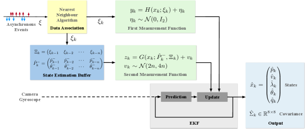
In this section, we present the proposed EKF-based asynchronous event blob tracker for event cameras (cf. Figure 3). We first present the EKF prediction step, before describing the measurement functions and the EKF update step. We will discuss the data association and other implementation details in the next section.
Recall the continuous-time system state (Equation 5) for . Define to be the estimated state and covariance of . The prediction step of our tracker is computed as a continuous-time diffusion associated with the stochastic differential equation (8), while the update step of our tracker is an asynchronous update based on pseudo measurements constructed from event data and undertaken when each new event becomes available, similar to [46, 47].
IV-A Asynchronous Object Dynamics and Prediction Step
The predicted state is computed by integrating the dynamics (8) without noise. We linearise the dynamics (8) about the predicted state in order to predict the covariance .
Linearising in Equation (7) about (the position components of ) yields
It follows that the dynamics of the true state , linearised about the estimated state , are
| (9) |
where is Wiener process with positive definite matrix
| (10) |
and the state matrix is a block matrix corresponding to the state partition of (5),
| (11) |
with as defined in (6). Note that, if is unavailable or zero (the camera is stationary), then . In this case, the dynamics (9) are exactly linear and are thus independent of the linearisation point ; that is, and does not depend on .
The state covariance , in the absence of measurements, is predicted as the solution of a continuous-time linear Gaussian diffusion process given by
| (12) |
where is computed around .
Let be a sequence of times associated with an event stream. For each given time , define the asynchronous system-state to be
| (13) |
Analogously, define asynchronous estimated state parameters at time . Given estimated state parameters at time the predicted state at time is the solution of (8) without noise for initial condition . The predicted covariance at time is the solution of (12) for initial condition . The actual computation of the prediction step used for the tracker algorithm is detailed in §V-E.
IV-B Two-Stage Pseudo Measurement Construction
Let be a sequence of events. The natural measurement available for event blob target tracking is the location of each event , available at discrete asynchronous times . The associated generative noise model for the raw event location measurement is given by (4). However, this model cannot be used directly in the proposed event-blob target tracking filter since the square-root uncertainty in the generative noise model is itself a state to be estimated by the filter (i.e., determined by variables in ). Instead, we will derive a pseudo measurement with known measurement covariance and use the theory of Kalman filtering with constraints [48].
Define a measurement function by
| (14) |
where is a function of the state parametrised by the measurement . Recalling (4), then by construction
where recall is an independent and identically distributed (i.i.d.) Gaussian process with known covariance. In particular, the expected value .
Define a new measurement model
| (15) |
with pseudo measurements . The generative noise model (15) with measurements has known stochastic parameters and can be used in a Kalman filter construction.
The measurement (15) is insufficient to provide observability of the full state . Intuitively, this can be seen by noting that a decreasing measurement error can be modelled either as indicating should be moved towards or that should be increased (see Figure 16 in the ablation study Section XI-B).
To overcome this issue, we introduce an additional pseudo measurement specifically designed to observe the shape parameter . The approach is to construct a chi-squared statistic from a buffer of prior state estimates that allows estimation of the shape parameters .
Assume that the extended Kalman filter has been operating for asynchronous iterations, with events received for the target. During initialisation we will run a bootstrap filter to generate an initial time-stamps to enable a warm start for the full filter. For a fixed index and window length , let and denote the state-estimate filter predictions based on measurements , where . Define to be the buffer of state prediction estimates
| (16) |
and to be the buffer of the associated events
| (17) |
For , define
| (18) |
where are the principal correlations at time , while the prior filter states are used to rotate the image moment to the best estimate of its orientation. Note that we do not use all the available data at time for the estimation of since doing so would introduce undesirable stochastic dependencies.
Let be a constant estimate of an over-bound for the uncertainty in . Define
| (19) |
Note that and . Replacing the estimates in (19) by their expected values yields a scaled version of the event generation model (4). Thus, the primary contribution to the uncertainty in will be a Gaussian distribution . Variance in is bounded by the estimated parameter . Since this variance has a similar structure to the variance in it can be approximated as contributing additional uncertainty to . The additional uncertainty in is only present in the rotation matrix and its contribution to uncertainty in is negligible. Thus, the uncertainty in can be modelled by
Define a new virtual output function
| (20) |
with dependence on through in (cf. Equation (19)). Since are normally distributed with unit covariance, the output function is the sum of the squares of independent 2-dimensional Gaussian random variables. Consequently, it follows a chi-squared distribution with an order of . According to the central limit theorem [49], as becomes sufficiently large, the chi-squared distribution converges to a normal distribution with a mean of and a variance of . Based on this, we propose a pseudo measurement model
| (21) |
with pseudo measurements .
This development depends on the bound . In practice, the uncertainty in is often much smaller compared to the uncertainty in the event position associated with the actual shape of the object. Typically is 100 to 1000 larger than , corresponding to a . Although this bound makes little difference in practice, it provides theoretical certainty that the filter will not become overconfident.
Define the combined virtual measurement
| (22) |
The expected value is for all by the definitions of and . Note that is a function of the (current) event and (current) state , while is a function only of the (past) events and the (past) filter estimate before the update step in the Kalman filter. It follows that the random variables in (15) and (21) are independent. This leads to the generative noise model
| (23) | |||||
| (24) | |||||
where and are independent.
IV-C EKF Update Step
We linearise the two non-linear measurement models and (15)-(21) by computing the Jacobian matrices of the and measurement functions. The linearised observation model for the state is written
| (25) | ||||
The detailed partial derivatives are provided in Appendix XI-A.
From here, we follow the standard extended Kalman filter algorithm to compute the pre-fit residual Kalman filter gain to be
| (26) |
Finally, the updated state estimate and covariance estimate are given by
| (27) | |||
| (28) |
V Implementation of Asynchronous Event Blob Tracker
In this section, we present the track initialisation, data association logic and other implementation details of the proposed AEB tracker.
V-A Track Initialisation
Following the precedent set by our primary comparison algorithms (ACE [50] and HASTE [23]), we use manual selection (click on screen) or predefined locations for specific experimental studies to initialise tracks in the suite of experimental studies documented in Section VI. In practice, the AEB tracker would be initialised using detection algorithms methodologies tailored to specific applications, such as high speed particle tracking [12] or eye tracking [14], which require specialised detection methodologies. There are a range of potential algorithms in the literature that could be used for this purpose [20, 16]. Further discussion of automated track initialisation is beyond the scope of the present paper.
We initialise targets with zero initial linear and angular velocity, and the initial target size is set to a value at least two times larger than the maximum expected blob size to make the initial transient of the filter more robust.
In addition to the initial states, the proposed filter requires estimates of process noise covariance and an initial prior for the state covariance. The tuning of these parameters follows standard practice for Kalman filter algorithms, allowing for data-based methods like Expectation Maximisation [51, 52]. Alternatively, manual tuning of process noise and prior covariances can be performed to align with the specific application and anticipated motion. The covariance prior for blob location and size is determined based on an estimation of the error in the blob detection methodology. The covariance for linear and angular velocity is set in an order of magnitude larger than the position estimate to allow the filter to quickly converge for these states. In cases of highly erratic motion, the value of can be increased to model stochastic variation in the linear optical flow of the target. For less erratic motions, can be decreased to enhance the algorithm’s resilience to outliers and noisy data. The better the predictive model of the motion of the target is, the smaller the value of can be made. In particular, when an IMU is present and ego-motion of the target for camera rotation can be estimated, this will tend to allow for significantly smaller and improve outlier rejection and robustness of the tracking performance. This is important since the ego-rotation of the camera generates the most spurious outlier events from the background texture. Default parameters for the covariance prior and that we have found to work well across a wide range of scenarios is documented in the companion code.
V-B Data Association
Data association in visual target tracking is arguably one of the most difficult problems. In this paper, we take a simple approach that considers all events in a neighbourhood of the event blob to be inliers. As long as the signal-to-noise ratio of the number of events generated by an event blob target to the background noise events is high enough, the disturbance from background noise events will be small and the filter will maintain track. Furthermore, any background noise events that are spatially homogeneous, such as an overall change of illumination, will be distributed in the developed pseudo measurements and will have only a marginal effect on the filter tracking performance. It is only when two objects generating a large number of events cross in the image that the algorithm may lose track. This may be due to two targets crossing in the image, such as when the tail lights from one car occlude the tail lights of another car. Or when the ego-motion of the camera causes a high-contrast background feature to cross behind a low-intensity target. Measuring camera ego-motion by an IMU and predicting the target’s position in the corresponding direction helps to address the second case.
There remains the question of choosing the neighbourhood in which to associate inliers and outliers. The size of this neighbourhood must be adapted dynamically to adjust for the changing size of the target in the image. Our data association approach uses the nearest neighbour classifier with a dynamic threshold . That is, any event that lies less than pixels from the predicted state estimate is associated with the target and used in the filter. The threshold is chosen as a low-pass version of . In continuous-time, this low-pass filer is written
| (29) |
where is the filter gain and is the desired ratio between the distance threshold and the estimated target size. Integrating (29) over the time interval for constant yields
| (30) | ||||
The gain is chosen based on the expected continuous-time dynamics of the target in the image.
V-C Multi-target Tracking
Our AEB tracker tracks multiple targets independently. Each target is updated as an individual state asynchronously as events arrive. This approach allows us to maintain separate and accurate tracking for multiple blob-like targets. When a target is detected a separate state model and the corresponding matrices (e.g., , , etc.,) is initialised for each new target as discussed in Section V-A. Events are processed asynchronously and assigned to separate targets using our data association method as discussed in Section V-B. These events are used to update the state of the associated target through our proposed algorithm. Any event not associated with a target is discarded.
V-D Non-flickering Object Tracking
 |
Flickering targets such as LED lights or non-flickering drones with spinning rotors trigger events that can be approximated to a spatial-temporal Gaussian event blob (Figure 2). However, a moving non-flickering object triggers a bimodal distribution of event data where the leading edge events have one polarity while the trailing edge events have the opposite polarity, depending on the intensity contrast of the blob to the background (see Figure 4). In this case, an unmodified version of the AEB tracker algorithm tends to track either the leading or trailing edge of the target and may sometimes switch between the two edges causing inconsistent velocity estimation. This behaviour only happens for non-flickering blob targets and arises because of the bimodal distribution of events.
To overcome this, we add a simple polarity offset parameter that models the pixel offset, with respect to a central point, between the leading and trailing edge polarity of the observed blob. We expand the state model to include the offset parameter. We add rotation dynamics with stochastic diffusion for the offset parameter to the state dynamics (8)
| (31) |
recalling from (6) and . The offset is used to compensate the event position in the first pseudo measurement function
| (32) |
where is the event polarity at event timestamp . Note that the polarity offset will converge to the corresponding direction as the velocity estimate if the blob is a light blob on a dark background and to the opposite direction to the velocity if it is a dark blob on a light background in order to balance the event polarities correctly. An analogous change is applied to the second pseudo measurement function (21).
V-E Prediction Step Integration
Since events are triggered in microsecond time resolution, the continuous-time prediction step in Equation (9)-(12) are well-approximated by a first-order Euler integration scheme. For each timestamp drawn from the events associated with a specific blob, define the time interval
| (33) |
The predicted estimate of the prior state and state covariance are computed by
| (34a) | ||||
| (34b) | ||||
V-F Computational Cost
The AEB tracker includes two main steps: data association and the extended Kalman filter. The data association step has a linear event complexity of for input events, effectively passing only a subset of events to the extended Kalman filter, where . The extended Kalman filter operates with a time complexity of , where denotes the buffer length in (16)-(17). In practice, the buffer length is typically set to , and it is worth noting that remains significantly larger than . As a result, our algorithm maintains an overall linear event complexity of .
Since the data association step only scales linearly with the event rate and this process significantly reduces the number of events used in the Extended Kalman filter, the algorithm is highly efficient for real-time implementation. The efficiency and asynchronous processing of the AEB tracker make it well-suited for implementation on FPGA. Such systems have the potential to be particularly advantageous for high-performance embedded robotic systems.
VI Experimental Evaluation
 |
This section is the first of two results sections. In this section we evaluate the AEB tracker in a controlled laboratory environments to provide comparative results to state-of-the-art event-based corner and blob tracking algorithms. Later, in Section VII we provide some real-world case studies. We provide two comparisons in this section; firstly tracking a spinning target to demonstrate the maximum optical flow that can be tracked, and secondly, tracking ego-motion of blobs for fast unstructured camera motion comparing tracking performance with and without IMU data.
VI-A Indoor Dataset Collection
For the ‘Fast-Spinning’ indoor experiment, we record high-resolution events using a Prophesee Gen4 pure event camera (7201280 pixels). We evaluate the tracking performance of different event-based corner and blob tracking algorithms at varying speeds. To achieve this, we have constructed a spinning disk test-bed (Figure 6) with adjustable spin rates, and we use a black square on a white disk as the target to provide corners for the corner detection algorithms to operate.
For the ‘Fast Moving Camera with Ego-motion’ experiment, we record data using a hybrid event-frame DAVIS 240C camera (180240 pixels) that outputs synchronised events, reference frames and IMU data. Note that we do not record frame data because the hybrid DAVIS cameras usually generate a large number of noisy events at the shutter time of each frame when operating in hybrid mode [55].
 |
 |
 |
| (a) | (b) | (c) |
VI-B Fast-Spinning Data
In this section, we evaluate our method against the most relevant state-of-the-art object-tracking algorithms that use only events as input, operate efficiently (preferably asynchronously), and require no training process. The comparisons include ACE from [50], four HASTE methods from [23], the generic object tracking method from the industrial Prophesee software [53] and the Rectangular Cluster Tracker (RCT) function from the jAER software [54]. In addition, we broaden our scope by comparing with event-based corner detection methods, including the popular asynchronous corner tracking algorithm Arc* [20] and the widely used benchmark method EOF [16]. Note that we limit our comparisons to event-based methods due to the extreme nature of our targeted scenarios in this paper. Frame-based cameras lack the capability to capture information for tracking fast motion or in poor lighting due to motion blur and jumps in blob location between frames (Fig. 6). All algorithms (where velocity is estimated) use a constant velocity model, that is, linear trajectories for the blobs. We do not provide algorithms with prior knowledge that the target trajectory is circular. This mismatch makes the dataset challenging at sufficiently high optical flow.
 |
| Algorithms | Max Speed (pixels/s) |
|---|---|
| ACE [50] | 914 |
| haste_correction [23] | 939 |
| haste_correction* [23] | 925 |
| haste_difference [23] | 992 |
| haste_difference* [23] | 1476 |
| Prophesee [53] | 2620 |
| jAER [54] | 9830 |
| AB_tracker (ours) | 11320 |
 |
The main panel of Figure 5 plots the -component of the blob position for each of the different algorithms during an experiment where the optical flow increases from 100 pixels/s to more than 11000 pixels/s over 90 seconds. The graphic above the main panel plots the period of time for which each algorithm provides reliable tracking of the blob. The plotted line indicates the period up to which the algorithm loses track the first time. The solid dot terminations indicate the end-of-life of the target track while the open circle terminations to the dotted line indicates that future tracks last less than one cycle. The bottom sub-figures highlight zooms of short windows of data to demonstrate key behaviour of the algorithms. The first window, at 1000 pixels/s, captures the moment when the ACE [50] and the four HASTE algorithms [23] begin to lose track. These algorithms have enduring state estimates and since the blob is travelling in a circular trajectory they often recapture the blob at a later moment as it recrosses the location of the state estimate. This intermittent tracking persists for some time but tracking failures become more regular and eventually the estimates drift from the circular route of the blob and tracking is lost. We also note that ACE [50] and HASTE [23] depend heavily on good identification of the feature template and this is only reliably possible at low speeds. The second figure captures the moment that the Prophesee [53] method loses track, while the third window captures the moment that the jAER [54] loses track. The Prophesee [53] was run with default parameters while the jAER [54] was hand-tuned working with the author (jAER [54]) to achieve the best performance on the test dataset possible. Both these algorithms delete target hypotheses when they lose track. This is indicated with a terminal point on the track in the zoomed windows. Both these algorithms also include detection routines and initialise new targets, which (if they happen to be the correct blob) are able to maintain track for a few additional cycles. However, the first tracking failure indicates the onset of non-robustness in the tracking. Both algorithms regularly lose track for optical flow higher than that indicated in the graphic above the main plot. Our proposed method continues to track stably up to the physical limitations of the experimental platform ( 6 rev/s). Table I presents the maximum optical flow that each algorithm could reliably maintain track.
In addition to the position estimation, jAER [54] and our proposed method also estimate the target velocity. In Figure 7, we plot the velocity estimates and of the target by the jAER [54] and our method. The figures illustrate the linear increase in peak velocity of the oscillation to around 11000 pixels/s in both the and directions. The two zoomed-in plots show the detailed behaviour of the velocity estimates of both algorithms for 9000 pixels/s and 11000 pixels/s and demonstrate the stability of our algorithm in comparison to the much noisier estimates provided by the jAER algorithm [54].
Apart from the blob tracking methods, we have also provided qualitative comparison studies with event-based corner detection methods, including the popular asynchronous corner tracking algorithm Arc* [20] and the widely used benchmark method EOF [16] at 1000 pixels/s and 9000 pixels/s is shown in Figure 8. We mark the corners detected by EOF [16] by green filled dots, Arc* [20] by magenta circles and the position estimated by our proposed method by an orange star. The two compared algorithms mostly detect corners around the target at low speed but fail at high speed and mainly detect the centre of the spinning test bed. Neither algorithm is able to provide reliable target tracking at high optical flow for this simple scenario.
 |
 |
|
 |
 |
|
| (a) no IMU | (b) with IMU (b) |
 |
VI-C Fast Moving Camera with Ego-motion
This section evaluates the effectiveness of compensating for camera ego-motion using IMU data in our tracker. The experiment involved tracking the black shapes on a white background in an image where the camera was rapidly shaken by hand. The dataset is similar to, and we used the same shapes image, as the popular dataset proposed by [56], but with more aggressive camera motions, and all targets remain in the camera field-of-view. Maximum optical flow rates are 1000 pixels/s with abrupt changes in direction.
In Figures 9 and 10, we compare the tracking trajectory of our AEB tracker with and without including camera ego-motion using IMU data. Brighter colours represent trajectories where no IMU data is available, while darker colours correspond to the case where gyroscope measurements from a camera-mounted IMU are available and used to predict ego-motion in the filter as outlined in Section IV. Figure 10 demonstrates that the ‘no IMU’ trajectories lag slightly behind those of the ego-motion compensated model. This effect is also visible in Fig. 9 where the position estimates of the ‘no IMU’ filter are lagging the latest event data slightly more than the estimates obtained using IMU to compensate ego-motion. Compensating camera ego-motion also reduces overshoot when the camera motion changes direction at high speed (Fig. 10). The combination of these effects makes the ‘no IMU’ case slightly less robust and we were able to induce a tracking failure when the camera was shaken at nearly 6Hz with optical flow rates between 1000 pixels/s. The authors note that although including camera ego-motion is clearly beneficial, the performance of the algorithm without ego-motion compensation is better than expected and is sufficient for many real-world applications.
 |
VII Real-World Case Study
In this section, we showcase our AEB tracker in two challenging real-world scenarios: tracking automotive tail light at night and tracking a quickly moving drone in complex environments, with applications to estimating time-to-contact and range estimation.
VII-A Outdoor Data Collection
Apart from recording event data using a Prophesee camera, we also use a FLIR RGB frame camera (Chameleon3USB3, 20481536 pixels) to capture high quality image frames for the real-world case study. The two cameras were placed side-by-side and time-synchronised by an external trigger (see Figure 13). The RGB camera frames were re-projected to the event camera image plane using stereo camera calibration. The re-projection mismatch due to the disparity between the two cameras is minor for far-away outdoor scenes. Both datasets include high-speed targets and challenging lighting conditions, allowing a comprehensive evaluation of tracking and shape estimation, as well as for downstream tasks such as time-to-contact estimation and range estimation. For the flying quadrotor dataset, we used a small quadrotor equipped with a Real-Time Kinematic (RTK) positioning GPS (see Figure 13).
VII-B Night Driving Experiment
In this experiment, the event camera system was mounted on a tripod (held down by hand in the foot well) inside a car driving on a public road at night. The proposed algorithm is used to track the tail lights of other vehicles, and we demonstrate its performance by using the output states to estimate time-to-contact (TTC) at more than 100kHz.
 |
 |
VII-B1 Time-To-Contact
Time-to-contact (TTC) defines the estimated time before a collision occurs between two objects, typically a vehicle and an obstacle or another vehicle. We estimate TTC by computing the rate of variation of the pixel distance between the left and right tail lights on the front cars in the image [58, 59]. Our filter provides high-rate estimates of the position and velocity of the event blobs associated with the left and right tail lights on each car at time , denoted as , , , and , respectively. The visual distance between the tail lights is defined to be
| (35) |
in pixels. The relative velocity between the left and right tail lights is defined to be the relative blob velocity in the direction of displacement (in pixels/s),
| (36) |
The TTC, measured in seconds, is the ratio of the visual distance between the left and right tail lights to the relative visual velocity between the lights on the same car in pixels [58, 59]
| (37) |
The inverse TTC
| (38) |
is most commonly used as a cue for obstacle avoidance since it is a bounded signal and setting warning thresholds is straightforward as shown in Figure 11.
VII-B2 Experiments
In Figure 11, we present an example of tracking the tail lights of three cars at night, travelling with an average speed of approximately 90 km/h. The figure displays the reference images captured by an RGB frame-based camera in (a) and the event reconstructions (obtained using the event high-pass filter [57]) in (b) across three different timestamps. Only the actual tail lights of the cars were tracked (marked with red ellipses on images (b)) and not the reflections of the tail lights visible in the bonnet of the car. By choosing the bias of the Prophesee Gen4 camera carefully, we are able to preserve events associated with the high-frequency LED lights and reduce background ego-motion events leading to high signal-to-noise event data. This trivialises the data association and enables robust, accurate, high-band width performance of our event blob tracker. Conversely, the RGB reference frames are mostly dark and blurry and obtaining dynamic information on relative motion in the image from this data would be difficult.
We estimate the inverse time-to-contact (TTC) of the left, middle, and right car separately and plot them in Figure 11c)-e). The timestamps corresponding to the RGB and event images in the top rows are marked in the plots below; timestamps (1), (2), and (3) are distinguished by a blue, orange, and pink dashed line, respectively. A positive indicates that the distance to a given car is decreasing, while a negative indicates that the distance to a given car is increasing (and consequently no collision can occur). For illustrative purposes, we have chosen to indicate a safety threshold at when the following car is around 3.3 seconds from collision with the leading car if the velocities were to be kept constant. Values exceeding this are shown in red in Figure 11c)-g).
Figure 11d) indicates the experimental vehicle maintaining a relatively constant TTC to the middle car in the same lane, consistent with safe driving margins. Figure 11e) shows the inverse TTC of the right car exceeds the safety threshold at approximately 4.3 seconds, shortly before we overtake it at 4.6 seconds. No TTC data is shown in Figure 11e) after 4.6 seconds since the car is not visible. In Figure 11c), the inverse TTC of the left car exceeds the safety threshold around 5 seconds. See the RGB frames and event reconstructions in Figure 11a)-b) for reference.
Irregularities in the road surface induce bouncing and swaying motion of the vehicle frame that, since the camera is held firmly to the dashboard of the car, lead to horizontal linear velocity of the camera and results in rapid changes in TTC. There are several clear short peaks in 11d), both positive and negative, due to small bumps and depressions in the road surface. For example, the brief 50-millisecond black (negative) peak that appears around 3.3 seconds in Figure 11d) along with the red peak in Figure 11e) would indicate that the left front wheel has encountered a bump inducing the vehicle to pitch backward and sway to the right. The motion can be appreciated in the supplementary video for the full sequence, although since the entire bump sequence occurs in a period of around 50ms the actual motion of the car is correspondingly small.
Figure 11f) provides a zoomed-in view of the red box section in Figure 11e) of 200 milliseconds in length, and Figure 11g) provides a further zoomed-in view of the yellow box section within subplot (f) of 4 milliseconds in length. These plots demonstrate the exceptionally high temporal resolution of our tracker, processing updates at more than 100kHz. This remarkable speed minimises latency for vital decision-making processes such as braking and acceleration, particularly in emergency situations. It clearly surpasses the capabilities of frame-based TTC algorithms, which are limited by the frequency of incoming RGB frames (typically around 40Hz), or even pseudo-frame event based algorithms (requiring around 1K to 10K events per pseudo-frame) that would operate in the order of 10-100Hz. This performance, for a single event camera at night and without any additional active sensors like Lidar or Radar, demonstrates the potential of applying event cameras, and the proposed AEB tracker, to problems in autonomous driving.
VII-C Flying Quadrotor Experiment
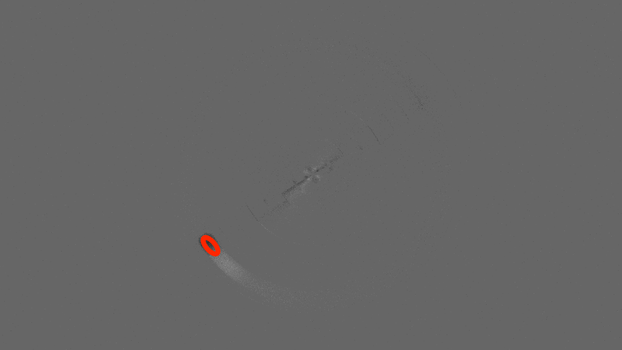
We demonstrate the performance of the proposed AEB tracker by tracking a flying quadrotor under various camera motions and lighting conditions shown in Figure 12. The average speed of the drone in the image is around 150 pixels/s, with some fast motions, such as fast flips, reaching speeds of 400 pixels/s. Figure 12a)-b) demonstrates the tracking performance in well-lit conditions, while data shown in Figure 12c)-d) demonstrate the performance in poorly lit conditions. The RGB images and event reconstruction images are provided for reference only and the filter is implemented on pure asynchronous event data. The red ellipses superimposed on the event reconstruction images illustrate the position, size, and orientation of the quadrotor as estimated by our AEB tracker. The minor axis of the ellipse aligns with the drone’s heading direction. Please also refer to the supplementary video to see the tracking performance.
The first two columns in Figure 12 show the reference frames and event reconstruction recorded with a stationary camera. In these conditions, the majority of the events are triggered by the movement of the quadrotor since it is the only object in the scene that changes brightness or motion. Therefore, the event reconstruction frames mainly consist of a gray background with an event blob triggered by the target. With good lighting conditions and a simple background, the target is easily distinguishable in both frames and event data (see Figure 12a). The advantage of our proposed algorithm over frame-based algorithms becomes more apparent in low-light conditions or environments with complex backgrounds. As shown in Figure 12b), the complex background in the frames makes tracking using RGB frames extremely challenging when the quadrotor crosses trees. In contrast, our AEB tracker can still track the quadrotor successfully. In the poorly lit sequences in Figure 12c)-d), the RGB frames only capture a faint green light emitted by an LED on the quadrotor, making tracking nearly impossible. On the other hand, the event camera can still capture unique event blobs of the quadrotor even in low light or in front of a complex background, providing sufficient information for our AEB tracker to achieve reliable tracking performance even in these challenging scenarios.
In the third column in Figure 12, when the camera is also moving, the background triggers many events, posing a challenge for tracking. The dynamic nearest neighbour data association approach (cf. Section V-B) selectively feeds events to the filter based on their proximity to the centre of the target and estimation of the target size. Only events within a dynamic threshold from the target’s centre are considered, effectively rejecting the vast majority of background noise. Although overall the tracking performance is excellent, the present algorithm can still lose track if substantial ego-motion of the camera occurs just as the target crosses a high contrast feature in the scene. This is particularly the case if the camera ego-motion tracks the target, since this reduces the optical flow of the target and increases the optical flow of the scene. In such situations, a scene feature blob can capture the filter state and draw it away from the target. Interestingly, this scenario is almost always related to the rotational ego-motion of the camera, since such motion generates the majority of optical flow in a scene. The corresponding filter velocity of the incorrect blob track could then be computed a-priori from the angular velocity of the camera, and this prior information could be exploited to reject false background tracks. Implementation of this concept is beyond the scope of the present paper but is relevant in the context of the future potential of the algorithm.
VII-C1 Qualitative Tracking Performance
To provide a qualitative measure of tracking performance we have overlaid the estimated trajectory of the tracked quadrotor on event reconstructions (obtained using the event-based high-pass filter [57]) during aerobatic manoeuvres. In Figure 14, red dots represent the continuous-time trajectory estimated by our AEB tracker while the background frames show the reconstructed intensity image from events. The close alignment between the red estimated trajectory and the observed event trajectory shows that our tracker accurately tracks the trajectory of the target quadrotor. The quadrotor was also equipped with RTK-GPS and the full 3D trajectory is shown as an orange trajectory in the perspective image in Figure 14. The corresponding zigzag and ‘E’ sub-trajectories are indicated in yellow. The camera position and East-North-Up direction are marked at the bottom right of the figure.
 |
VII-C2 Range Estimation
The shape parameters estimated in the proposed filter allow us to derive an estimate of range for a target with known size. The target shape parameters encode the visual second-order moment of the event blob. Since the quadrotor is disc shaped, the maximum of the visual second-order moment is visually related to the diameter of the quadrotor. By triangulation, the range can be estimated by
| Range | (39) |
where is the actual diameter of the target in meters and is the camera focal length. Note that we estimate the real-world target range based on the object’s real-world size and the camera’s focal length as prior knowledge, assuming the target size is constant.
We provide an example of range estimation for a quadrotor as it approaches the camera location in low-light conditions from a distance of approximately 17 meters to a distance of less than 8 meters in Figure 15. The image data is shown at three time-stamps each indicated by a different colour while the detailed range estimation data is shown in red in the following graph. The reference data points (in blue) are computed from RTK-GPS log from the vehicle compared to a known GPS location of the camera. Note that the RTK-GPS is only available at 5Hz and our AEB tracker achieves more than a 50kHz update.
The quadrotor is almost impossible to visually identify or track using the dark RGB images in Figure 15. This is particularly the case when it flies in front of the dark mountains in the background. The precision of the proposed range information is strongly coupled with the high filter update rates that allow for temporal smoothing of the inferred shape parameters. In particular, even though the virtual measurement function based on the chi-squared statistic does involve temporal averaging, the time window on which this statistic is computed is so short (due to the high filter update rate) compared to the vehicle dynamics that the proposed range estimate is remarkably reliable.
 |
VIII Limitations and Future Works
The proposed algorithm uses a simple and computationally efficient data association method that is suitable for many general tasks. However, this simplicity limits its application in tasks with crossing targets and large amounts of extraneous events generated by textured background and ego-motion of the camera. Future research avenues include the design of a more robust data association algorithm for general tasks and the creation of specific data association methods tailored to specialised tasks that are robust to ego-motion. A second avenue for further work is to develop a robust detection method method and building a complete detection and tracking system to complement the spatio-temporal Gaussian likelihood model for event blob target tracking. Finally, it is of interest to extend the approach track general spatio-temporal features rather than just blobs.
IX Conclusion
This paper presents a novel asynchronous event blob tracker for tracking event blobs in real time. The proposed filter achieves accurate tracking and blob shape estimation even under low-light environments and high-speed motion. It fully exploits the advantages of events by processing each event and updating the filter state asynchronously, achieving high temporal resolution state estimation (over 50kHz for the experiments undertaken). The algorithm outperforms state-of-the-art event tracking algorithms in laboratory based experimental testing, achieving tracking rates in excess of 11000 pixels/s. The high-rate, robust filter output directly enables downstream tasks such as range estimation and time-to-contact in autonomous driving, demonstrating the practical potential of the algorithm in a wide range of computer vision and robotics applications that require precise tracking and size estimation of fast-moving targets.
 |
 |
 |
 |
 |
|
 |
 |
 |
 |
 |
|
X Acknowledgement
The authors would like to thank Professor Tobias Delbruck of ETH Zurich for his guidance in using and tuning parameters within the jAER software [54], along with his insightful suggestions to this paper. We also sincerely thank Dr. Andrew Tridgell and Ms. Michelle Rossouw from the Ardupilot Community for their invaluable help collecting and processing the quadrotor dataset. We thank Dr. Iain Guilliard and Mr. Angus Apps from the Australian National University for their contributions in modularising the codebase to enhance accessibility.
XI Appendix
XI-A Partial Derivatives of Observation Model
The partial derivatives of with respect to , and are given by
| (40) | ||||
The partial derivatives of with respect to , and are given by
| (41) | ||||
where
| (42) | ||||
XI-B Ablation Study
In this section we present an ablation study to evaluate the effectiveness of our second measurement function in the combined measurement function (22) and experimentally demonstrate that adding enhances the observability of the shape parameter , as discussed in Section IV-B.
We use the ‘Fast-Spinning’ dataset for this comparison. Figure 16 illustrates the size estimation and tracking performance of using the combined measurement function in (a) and using only the first measurement function in (b). The background intensity is generated using high-pass filter [57] for display only. The estimated target position and size are marked by red ellipses.
We initialise the target position and size at timestamp . After 0.2 milliseconds, the ellipse computed by the combined measurement function in (a) quickly shrinks to the corresponding target size, while the ellipse of using the single measurement in (b) remains almost unchanged. Subsequently, the ellipse in (a) further shrinks to the actual target size and the filter tracks the moving target accurately. However, the ellipse in (b) using only the first measurement function , tracks the target but demonstrates a gradual increase in estimated size and eventually loses track.
References
- [1] G. Gallego, T. Delbrück, G. Orchard, C. Bartolozzi, B. Taba, A. Censi, S. Leutenegger, A. J. Davison, J. Conradt, K. Daniilidis, and D. Scaramuzza, “Event-based vision: A survey,” IEEE transactions on pattern analysis and machine intelligence, vol. 44, no. 1, pp. 154–180, 2020.
- [2] J. N. P. Martel, J. Müller, J. Conradt, and Y. Sandamirskaya, “An active approach to solving the stereo matching problem using event-based sensors,” in IEEE Int. Symp. Circuits Syst. (ISCAS), 2018, pp. 1–5.
- [3] Z. Wang, Y. Ng, P. van Goor, and R. Mahony, “Event camera calibration of per-pixel biased contrast threshold,” Australasian Conference on Robotics and Automation, ACRA, 2019.
- [4] M. Litzenberger, C. Posch, D. Bauer, A. N. Belbachir, P. Schön, B. Kohn, and H. Garn, “Embedded vision system for real-time object tracking using an asynchronous transient vision sensor,” in Digital Signal Processing Workshop, 2006, pp. 173–178.
- [5] T. Delbruck and P. Lichtsteiner, “Fast sensory motor control based on event-based hybrid neuromorphic-procedural system,” in IEEE Int. Symp. Circuits Syst. (ISCAS), 2007, pp. 845–848.
- [6] T. Delbruck and M. Lang, “Robotic goalie with 3ms reaction time at 4% CPU load using event-based dynamic vision sensor,” Front. Neurosci., vol. 7, p. 223, 2013.
- [7] T. Chin, S. Bagchi, A. P. Eriksson, and A. van Schaik, “Star tracking using an event camera,” in IEEE Conf. Comput. Vis. Pattern Recog. Workshops (CVPRW), 2019.
- [8] T. Chin and S. Bagchi, “Event-based star tracking via multiresolution progressive hough transforms,” in IEEE Winter Conf. Appl. Comput. Vis. (WACV), 2020.
- [9] Y. Ng, Y. Latif, T.-J. Chin, and R. Mahony, “Asynchronous kalman filter for event-based star tracking,” in Computer Vision–ECCV 2022 Workshops: Tel Aviv, Israel, October 23–27, 2022, Proceedings, Part I. Springer, 2023, pp. 66–79.
- [10] Z. Ni, C. Pacoret, R. Benosman, S.-H. Ieng, and S. Régnier, “Asynchronous event-based high speed vision for microparticle tracking,” J. Microscopy, vol. 245, no. 3, pp. 236–244, 2012.
- [11] D. Drazen, P. Lichtsteiner, P. Häfliger, T. Delbrück, and A. Jensen, “Toward real-time particle tracking using an event-based dynamic vision sensor,” Experiments in Fluids, vol. 51, no. 5, pp. 1465–1469, 2011.
- [12] Y. Wang, R. Idoughi, and W. Heidrich, “Stereo event-based particle tracking velocimetry for 3d fluid flow reconstruction,” in Computer Vision–ECCV 2020: 16th European Conference, Glasgow, UK, August 23–28, 2020, Proceedings, Part XXIX 16. Springer, 2020, pp. 36–53.
- [13] A. N. Angelopoulos, J. N. Martel, A. P. Kohli, J. Conradt, and G. Wetzstein, “Event-based near-eye gaze tracking beyond 10,000 hz,” IEEE Transactions on Visualization and Computer Graphics, vol. 27, no. 5, pp. 2577–2586, 2021.
- [14] C. Ryan, B. O’Sullivan, A. Elrasad, A. Cahill, J. Lemley, P. Kielty, C. Posch, and E. Perot, “Real-time face & eye tracking and blink detection using event cameras,” Neural Networks, vol. 141, pp. 87–97, 2021.
- [15] A. Z. Zhu, N. Atanasov, and K. Daniilidis, “Event-based visual inertial odometry,” in IEEE Conf. Comput. Vis. Pattern Recog. (CVPR), 2017, pp. 5816–5824.
- [16] ——, “Event-based feature tracking with probabilistic data association,” in IEEE Int. Conf. Robot. Autom. (ICRA), 2017, pp. 4465–4470.
- [17] J. Manderscheid, A. Sironi, N. Bourdis, D. Migliore, and V. Lepetit, “Speed invariant time surface for learning to detect corner points with event-based cameras,” in IEEE Conf. Comput. Vis. Pattern Recog. (CVPR), 2019.
- [18] S. Hu, Y. Kim, H. Lim, A. J. Lee, and H. Myung, “ecdt: Event clustering for simultaneous feature detection and tracking,” in 2022 IEEE/RSJ International Conference on Intelligent Robots and Systems (IROS). IEEE, 2022, pp. 3808–3815.
- [19] X. Clady, S.-H. Ieng, and R. Benosman, “Asynchronous event-based corner detection and matching,” Neural Netw., vol. 66, pp. 91–106, 2015.
- [20] I. Alzugaray and M. Chli, “Asynchronous corner detection and tracking for event cameras in real time,” IEEE Robotics and Automation Letters, vol. 3, no. 4, pp. 3177–3184, 2018.
- [21] F. Barranco, C. Fermuller, and E. Ros, “Real-time clustering and multi-target tracking using event-based sensors,” in 2018 IEEE/RSJ International Conference on Intelligent Robots and Systems (IROS). IEEE, 2018, pp. 5764–5769.
- [22] R. Li, D. Shi, Y. Zhang, K. Li, and R. Li, “Fa-harris: A fast and asynchronous corner detector for event cameras,” in 2019 IEEE/RSJ International Conference on Intelligent Robots and Systems (IROS). IEEE, 2019, pp. 6223–6229.
- [23] I. Alzugaray and M. Chli, “Haste: multi-hypothesis asynchronous speeded-up tracking of events,” in 31st British Machine Vision Virtual Conference (BMVC 2020). ETH Zurich, Institute of Robotics and Intelligent Systems, 2020, p. 744.
- [24] J. Duo and L. Zhao, “An asynchronous real-time corner extraction and tracking algorithm for event camera,” Sensors, vol. 21, no. 4, p. 1475, 2021.
- [25] D. Gehrig, H. Rebecq, G. Gallego, and D. Scaramuzza, “EKLT: Asynchronous photometric feature tracking using events and frames,” Int. J. Comput. Vis., 2019.
- [26] E. Mueggler, N. Baumli, F. Fontana, and D. Scaramuzza, “Towards evasive maneuvers with quadrotors using dynamic vision sensors,” in 2015 European Conference on Mobile Robots (ECMR). IEEE, 2015, pp. 1–8.
- [27] A. Mitrokhin, C. Fermuller, C. Parameshwara, and Y. Aloimonos, “Event-based moving object detection and tracking,” in IEEE/RSJ Int. Conf. Intell. Robot. Syst. (IROS), 2018.
- [28] D. Falanga, S. Kim, and D. Scaramuzza, “How fast is too fast? the role of perception latency in high-speed sense and avoid,” IEEE Robotics and Automation Letters, vol. 4, no. 2, pp. 1884–1891, 2019.
- [29] D. Falanga, K. Kleber, and D. Scaramuzza, “Dynamic obstacle avoidance for quadrotors with event cameras,” Science Robotics, vol. 5, no. 40, p. eaaz9712, 2020.
- [30] N. J. Sanket, C. M. Parameshwara, C. D. Singh, A. V. Kuruttukulam, C. Fermüller, D. Scaramuzza, and Y. Aloimonos, “Evdodgenet: Deep dynamic obstacle dodging with event cameras,” in 2020 IEEE International Conference on Robotics and Automation (ICRA). IEEE, 2020, pp. 10 651–10 657.
- [31] J. P. Rodríguez-Gómez, A. G. Eguíluz, J. Martínez-de Dios, and A. Ollero, “Asynchronous event-based clustering and tracking for intrusion monitoring in uas,” in 2020 IEEE International Conference on Robotics and Automation (ICRA). IEEE, 2020, pp. 8518–8524.
- [32] H. Li and L. Shi, “Robust event-based object tracking combining correlation filter and cnn representation,” Frontiers in neurorobotics, vol. 13, p. 82, 2019.
- [33] H. Chen, Q. Wu, Y. Liang, X. Gao, and H. Wang, “Asynchronous tracking-by-detection on adaptive time surfaces for event-based object tracking,” in Proceedings of the 27th ACM International Conference on Multimedia, 2019, pp. 473–481.
- [34] B. Ramesh, S. Zhang, Z. W. Lee, Z. Gao, G. Orchard, and C. Xiang, “Long-term object tracking with a moving event camera,” in British Mach. Vis. Conf. (BMVC), 2018.
- [35] H. Chen, D. Suter, Q. Wu, and H. Wang, “End-to-end learning of object motion estimation from retinal events for event-based object tracking,” in Proceedings of the AAAI Conference on Artificial Intelligence, vol. 34, no. 07, 2020, pp. 10 534–10 541.
- [36] J. Zhang, B. Dong, H. Zhang, J. Ding, F. Heide, B. Yin, and X. Yang, “Spiking transformers for event-based single object tracking,” in Proceedings of the IEEE/CVF conference on Computer Vision and Pattern Recognition, 2022.
- [37] Z. Zhu, J. Hou, and X. Lyu, “Learning graph-embedded key-event back-tracing for object tracking in event clouds,” Advances in Neural Information Processing Systems, vol. 35, pp. 7462–7476, 2022.
- [38] N. Messikommer*, C. Fang*, M. Gehrig, and D. Scaramuzza, “Data-driven feature tracking for event cameras,” IEEE Conference on Computer Vision and Pattern Recognition, 2023.
- [39] J. Zhang, X. Yang, Y. Fu, X. Wei, B. Yin, and B. Dong, “Object tracking by jointly exploiting frame and event domain,” in Proceedings of the IEEE/CVF International Conference on Computer Vision, 2021, pp. 13 043–13 052.
- [40] C. Iaboni, D. Lobo, J.-W. Choi, and P. Abichandani, “Event-based motion capture system for online multi-quadrotor localization and tracking,” Sensors, vol. 22, no. 9, p. 3240, 2022.
- [41] G. R. Müller and J. Conradt, “A miniature low-power sensor system for real time 2d visual tracking of led markers,” in 2011 IEEE International Conference on Robotics and Biomimetics. IEEE, 2011, pp. 2429–2434.
- [42] A. Censi, J. Strubel, C. Brandli, T. Delbruck, and D. Scaramuzza, “Low-latency localization by active LED markers tracking using a dynamic vision sensor,” in IEEE/RSJ Int. Conf. Intell. Robot. Syst. (IROS), 2013.
- [43] Z. Wang, Y. Ng, J. Henderson, and R. Mahony, “Smart visual beacons with asynchronous optical communications using event cameras,” in ”International Conference on Intelligent Robots and Systems (IROS 2022)”, 2022.
- [44] Z. Wang, D. Yuan, Y. Ng, and R. Mahony, “A linear comb filter for event flicker removal,” in ”International Conference on Robotics and Automation (ICRA)”, 2022.
- [45] P. I. Corke, W. Jachimczyk, and R. Pillat, Robotics, vision and control: fundamental algorithms in MATLAB. Springer, 2011, vol. 73.
- [46] Z. Wang, Y. Ng, C. Scheerlinck, and R. Mahony, “An asynchronous kalman filter for hybrid event cameras,” in Int. Conf. Comput. Vis. (ICCV), 2021.
- [47] ——, “An asynchronous linear filter architecture for hybrid event-frame cameras,” IEEE Transactions on Pattern Analysis and Machine Intelligence, 2023.
- [48] S. J. Julier and J. J. LaViola, “On kalman filtering with nonlinear equality constraints,” IEEE transactions on signal processing, vol. 55, no. 6, pp. 2774–2784, 2007.
- [49] G. E. Box, W. H. Hunter, S. Hunter et al., Statistics for experimenters. John Wiley and sons New York, 1978, vol. 664.
- [50] I. Alzugaray and M. Chli, “ACE: An efficient asynchronous corner tracker for event cameras,” in 3D Vision (3DV), 2018, pp. 653–661.
- [51] R. H. Shumway, D. S. Stoffer, and D. S. Stoffer, Time series analysis and its applications. Springer, 2000, vol. 3.
- [52] E. E. Holmes, “Derivation of an em algorithm for constrained and unconstrained multivariate autoregressive state-space (marss) models,” arXiv preprint arXiv:1302.3919, 2013.
- [53] “Prophesee Software Tool for Generic Object Tracking,” https://docs.prophesee.ai/stable/samples/modules/analytics/tracking_generic_cpp.html, accessed on: .
- [54] “jAER Open Source Project: Java tools for Address-Event Representation (AER) neuromorphic processing,” https://github.com/SensorsINI/jaer, 2007, accessed on: .
- [55] Z. Wang, L. Pan, Y. Ng, Z. Zhuang, and R. Mahony, “Stereo hybrid event-frame (shef) cameras for 3d perception,” in 2021 IEEE/RSJ International Conference on Intelligent Robots and Systems (IROS). IEEE, 2021, pp. 9758–9764.
- [56] E. Mueggler, H. Rebecq, G. Gallego, T. Delbruck, and D. Scaramuzza, “The event-camera dataset and simulator: Event-based data for pose estimation, visual odometry, and SLAM,” Int. J. Robot. Research, vol. 36, no. 2, pp. 142–149, 2017.
- [57] C. Scheerlinck, N. Barnes, and R. Mahony, “Continuous-time intensity estimation using event cameras,” in Asian Conference on Computer Vision. Springer, 2018, pp. 308–324.
- [58] A. Negre, C. Braillon, J. L. Crowley, and C. Laugier, “Real-time time-to-collision from variation of intrinsic scale,” in Experimental Robotics: The 10th International Symposium on Experimental Robotics. Springer, 2008, pp. 75–84.
- [59] S. Gonner, D. Muller, S. Hold, M. Meuter, and A. Kummert, “Vehicle recognition and ttc estimation at night based on spotlight pairing,” in 2009 12th International IEEE Conference on Intelligent Transportation Systems. IEEE, 2009, pp. 1–6.
XII Biography Section
![[Uncaptioned image]](https://cdn.awesomepapers.org/papers/fedbef22-994a-4f3d-8e37-4443e538a3b0/ziwei.png) |
Ziwei Wang is a Ph.D. student in the Systems Theory and Robotics (STR) group at the College of Engineering and Computer Science, Australian National University (ANU), Canberra, Australia. She received her B.Eng degree from ANU (Mechatronics) in 2019. Her interests include event-based vision, asynchronous image processing and robotic applications. She is an IEEE student member. |
![[Uncaptioned image]](https://cdn.awesomepapers.org/papers/fedbef22-994a-4f3d-8e37-4443e538a3b0/timothy-molloy.jpg) |
Timothy L. Molloy (Member, IEEE) was born in Emerald, Australia. He received the BE and PhD degrees from the Queensland University of Technology (QUT) in 2010 and 2015, respectively. He is currently a Senior Lecturer in the School of Engineering at the Australian National University (ANU). Prior to joining ANU, he was an Advance Queensland Research Fellow at QUT (2017-2019), and a Research Fellow at the University of Melbourne (2020-2022). His interests include signal processing and information theory for robotics and control. Dr. Molloy is the recipient of a QUT University Medal, a QUT Outstanding Doctoral Thesis Award, a 2018 Boeing Wirraway Team Award, and an Advance Queensland Early-Career Fellowship. |
![[Uncaptioned image]](https://cdn.awesomepapers.org/papers/fedbef22-994a-4f3d-8e37-4443e538a3b0/PieterZoomed.jpg) |
Pieter van Goor is a research fellow at the Australian National University. He received the BEng(R&D)/BSc (2018) and Ph.D. (Engineering) (2023) degrees from the Australian National University . His research interests include applications of Lie group symmetries and geometric methods to problems in control and robotics, and in particular visual spatial awareness. He is an IEEE member. |
![[Uncaptioned image]](https://cdn.awesomepapers.org/papers/fedbef22-994a-4f3d-8e37-4443e538a3b0/Rob_photo.jpg) |
Robert Mahony (Fellow, IEEE) is a Professor in the School of Engineering at the Australian National University. He is the lead of the Systems Theory and Robotics (STR) group. He received his BSc in 1989 (applied mathematics and geology) and his PhD in 1995 (systems engineering) both from the Australian National University. He is a fellow of the IEEE. His research interests are in non-linear systems theory with applications in robotics and computer vision. He is known for his work in aerial robotics, geometric observer design, robotic vision, and optimisation on matrix manifolds. |