This paper was converted on www.awesomepapers.org from LaTeX by an anonymous user.
Want to know more? Visit the Converter page.

Asymptotic theory of CC-pseudo-cones111This paper was supported by the NSFC (No. 12371060), the Shaanxi Fundamental Science Research Project for Mathematics and Physics (No. 22JSZ012) and the Excellent Graduate Training Program of SNNU (No. LHRCCX23142).

Xudong Wang, Wenxue Xu, Jiazu Zhou, Baocheng Zhu
Abstract

In this paper, we study the non-degenerated CC-pseudo-cones which can be uniquely decomposed into the sum of a CC-asymptotic set and a CC-starting point. Combining this with the novel work in [34], we introduce the asymptotic weighted co-volume functional TΘ(E)T_{\Theta}(E) of the non-degenerated CC-pseudo-cone EE, which is also a generalized function with the singular point oo (the origin). Using our convolution formula for TΘ(E)T_{\Theta}(E), we establish a decay estimate for TΘ(E)T_{\Theta}(E) at infinity and present some interesting results. As applications of this asymptotic theory, we prove a weighted Brunn-Minkowski type inequality and study the solutions to the weighted Minkowski problem for pseudo-cones. Moreover, we pose an open problem regarding TΘ(E)T_{\Theta}(E), which we call the asymptotic Brunn-Minkowski inequality for CC-pseudo-cones.

Mathematics Subject Classification 2020. 52A30, 52A39, 52A40.

Keywords. CC-pseudo-cone, CC-starting point, asymptotic weighted co-volume, Brunn-Minkowski type inequality.

1 Introduction

The polar operator on the space 𝒦n\mathscr{K}^{n} of convex bodies and its functional counterpart, the Legendre transform on the class Cvx(n)\text{Cvx}(\mathbb{R}^{n}) of lower semi-continuous convex functions, play an important role in convex geometry, see [28] for more details. As an abstraction, an order reversing involution on certain partially ordered sets is called a duality. All dualities on 𝒦n\mathscr{K}^{n} and Cvx(n)\text{Cvx}(\mathbb{R}^{n}) are completely characterized by the polar operator [8] and the Legendre transform [4], respectively. In [3, 5], Artstein-Avidan and Milman introduced a new duality transform that is different from the Legendre transform on the sub-class Cvx0(n)\text{Cvx}_{0}(\mathbb{R}^{n}) (the class of geometric convex functions) of Cvx(n)\text{Cvx}(\mathbb{R}^{n}). Naturally, a question arises: what is the geometric version corresponding to this new duality transform? In a special case, Rashkovskii [27] studied the copolarity of coconvex sets in the positive orthant of n\mathbb{R}^{n}. Later, Artstein-Avidan, Sadovsky and Wyczesany [6] pointed out that all order reversing quasi-involutions can be induced by a cost function and exhibited various attractive dualities. Moreover, they systematically studied this geometric version of the new duality transform (termed dual polarity) and showed that the acting object of the dual polarity is a cone-like unbounded closed convex set. They also established the Blaschke-Santaló type inequality for the cone-like sets under the condition of essential symmetry. The cone-like set and dual polarity were further examined in [42], where the authors referred to this cone-like set as the pseudo-cone.

On the other hand, inspired by the works of Khovanskii and Timorin [19] and Milman and Rotem [25], Schneider [30] established the Brunn-Minkowski theory for CC-close sets, where CC is a pointed closed convex cone in n\mathbb{R}^{n}. Similar to the dual Minkowski problem posed by Huang, Lutwak, Yang and Zhang [16] for convex bodies, Li, Ye and the fourth author [22] introduced the concept of CC-compatible sets and studied their copolarity to address the dual Minkowski problem for unbounded closed convex sets. Adopting terms and conventions from [33, 34], these related results have shown that dual polarity is equivalent to copolarity and that CC-compatible sets are the same as CC-pseudo-cones. Quite recently, Semenov and Zhao [37] studied some characterizations of the CC-asymptotic sets to solve the Minkowski problem for the CC-asymptotic sets given by the infinity measure. Inspired by these, our first result in this paper is a classification of CC-pseudo-cones. That is, a non-degenerated CC-pseudo-cone can be uniquely decomposed into the sum of a CC-asymptotic set and a point in CC. To state this result precisely, we gather some foundational concepts, which can be found in [6, 22, 30, 33, 34, 35, 42].

Denote by ,\langle\cdot,\cdot\rangle and |||\cdot| the inner product and norm in n\mathbb{R}^{n}, respectively. We write B2nB_{2}^{n} and 𝕊n1\mathbb{S}^{n-1} for the unit ball and the unit sphere in n\mathbb{R}^{n}, respectively. The topological boundary and the topological interior of a subset EnE\subset\mathbb{R}^{n} are denoted by E\partial E and intE\text{int}\,E, respectively. Denote by HuH_{u}^{-} a negative half-space with the outer normal vector u𝕊n1u\in\mathbb{S}^{n-1}. Let CC be a pointed closed convex cone in n\mathbb{R}^{n} with non-empty interior, i.e., CC is a nn-dimensional closed convex cone that is line-free. The polar cone of CC is defined by C={yn|x,y0,xC}C^{\circ}=\{y\in\mathbb{R}^{n}\,|\,\langle x,y\rangle\leqslant 0,\,\forall\,x\in C\}, which is also line-free. Denote by ΩC=𝕊n1intC\Omega_{C}=\mathbb{S}^{n-1}\cap\text{int}\,C and ΩC=𝕊n1intC\Omega_{C^{\circ}}=\mathbb{S}^{n-1}\cap\text{int}\,C^{\circ}. Let o𝔸Co\notin\mathbb{A}\subset C be an unbounded closed convex set and A=C𝔸A=C\setminus\mathbb{A}. If AA has finite volume, then 𝔸\mathbb{A} is called a CC-close set and AA is called a CC-coconvex set. Specifically, a CC-close set 𝔸\mathbb{A} is called a CC-full set if AA is bounded. Moreover, 𝔸\mathbb{A} is called a CC-asymptotic set if 𝔸\mathbb{A} is asymptotic to C\partial C at infinity, i.e.,

limx𝔸,|x|+d(x,C)=0,\lim_{x\in\partial\mathbb{A},|x|\rightarrow+\infty}d(x,\partial C)=0, (1)

where d(x,C)d(x,\partial C) is the distance from xx to C\partial C. Let EnE\subset\mathbb{R}^{n} be a non-empty closed convex set. The recession cone of EE is defined by recE={xn|E+xE}{\rm rec}\,E=\{x\in\mathbb{R}^{n}\,|\,E+x\subset E\}. If EE is unbounded, then recE{\rm rec}\,E is a closed convex cone. Let oEno\notin E\subset\mathbb{R}^{n} be a non-empty closed convex set, EE is called a pseudo-cone if there holds λxE\lambda x\in E for any λ1\lambda\geqslant 1 and xEx\in\,E. For an nn-dimensional pointed closed convex cone CC, if EE is a pseudo-cone and recE=C{\rm rec}\,E=C, then EE is called a CC-pseudo-cone.

Now, we present a asymptotic characterization for the CC-pseudo-cones. For the definition of the support function of CC-pseudo-cones, please see (3).

Theorem 1.

Let CC be a pointed closed convex cone in n\mathbb{R}^{n} with non-empty interior and oEno\notin E\subset\mathbb{R}^{n} be a CC-pseudo-cone, then the following two statements are equivalent:
(i)(i) There is a point zCz\in C such that hE(v)=z,vh_{E}(v)=\langle z,v\rangle for all vΩCv\in\partial\Omega_{C^{\circ}};
(ii)(ii) EE can be uniquely decomposed into E=z+𝔸E=z+\mathbb{A}, where 𝔸\mathbb{A} is a CC-asymptotic set and zCz\in C.

We call a CC-pseudo-cone satisfying (i)(i) or (ii)(ii) in Theorem 1 as a non-degenerated CC-pseudo-cone. Moreover, for a non-degenerated CC-pseudo-cone E=z+𝔸E=z+\mathbb{A}, we call zz as the CC-starting point of EE and z+Cz+C as the asymptotic cone of EE. If z=oz=o, then Theorem 1 reduces to Theorem 2.6 in [37]. But the methods in this paper are different from [37]. There is a beautiful example of the degenerated CC-pseudo-cone proposed by Schneider in high dimension (n3n\geqslant 3), please see Figure 1 in Section 3. Furthermore, from a new perspective, the CC-starting point of a non-degenerated CC-pseudo-cone can offer insights into the conic linear bundle. As applications of this asymptotic theory of CC-pseudo-cones, one can establish a strengthened version of the Brunn-Minkowski inequality for CC-coconvex sets [30], see Section 6 for details.

Since the main behavior of a CC-pseudo-cone concentrates around the origin, i.e., all CC-pseudo-cones have almost same asymptotic behavior at infinity, the usual Lebesgue measure space is not suitable for CC-pseudo-cones. Following Schneider’s idea on the finiteness of the measure [34], one can endow a weight on CC to ensure the compactness for CC-pseudo-cones. Throughout this paper, we denote the weight function by Θ:C{o}(0,)\Theta:C\setminus\{o\}\rightarrow(0,\infty), which is a (q)(-q)-homogeneous continuous function with qq\in\mathbb{R}. A good example of such a weight function is Θ(y)=|y|q\Theta(y)=|y|^{-q} for any yC{o}y\in C\setminus\{o\}.

The weighted surface area measure [34] of EE is given by the push-forward measure of the weighted boundary Hausdorff measure, specifically,

Sn1Θ(E,)=𝝂EΘ(n1eE),S^{\Theta}_{n-1}(E,\cdot)={\boldsymbol{\nu}_{E}}_{\sharp}\,\Theta(\mathscr{H}^{n-1}\llcorner\partial_{e}E),

where 𝝂E\boldsymbol{\nu}_{E} is the Gauss image of EE and eE=Ecl(CE)\partial_{e}E=E\cap\text{cl}\,(C\setminus E) is the effective boundary of EE (see [22] or section 2 for more details). Schneider [34] showed that for q>n1q>n-1 and every CC-pseudo-cone EE, Sn1Θ(E,)S^{\Theta}_{n-1}(E,\cdot) is finite. Moreover, the weighted volume VΘ(E)V_{\Theta}(E) and the weighted co-volume V¯Θ(E)\overline{V}_{\Theta}(E) of CC-pseudo-cone EE are defined as follows:

VΘ(E)=EΘ(x)𝑑n(x),V¯Θ(E)=CEΘ(x)𝑑n(x).V_{\Theta}(E)=\int_{E}\Theta(x)\,d\mathscr{H}^{n}(x),\quad\overline{V}_{\Theta}(E)=\int_{C\setminus E}\Theta(x)\,d\mathscr{H}^{n}(x).

Schneider [34] also proved that for any n1<q<nn-1<q<n and every CC-pseudo-cone EE, V¯Θ(E)\overline{V}_{\Theta}(E) is finite.

From the asymptotic perspective of a CC-pseudo-cone, we define the asymptotic weighted co-volume functional of non-degenerated CC-pseudo-cones as follows: Let zz be the CC-starting point of the CC-pseudo-cone EE, expressed as E=z+𝔸E=z+\mathbb{A} for some CC-asymptotic set 𝔸\mathbb{A}. The asymptotic weighted co-volume of EE is defined by

TΘ(E)=TΘ(𝔸,z)=(z+C)EΘ(x)𝑑n(x).T_{\Theta}(E)=T_{\Theta}(\mathbb{A},z)=\int_{(z+C)\setminus E}\Theta(x)\,d\mathscr{H}^{n}(x).

We can view this asymptotic weighted co-volume TΘ(E)T_{\Theta}(E) as a functional of two variables. If we fix a CC-asymptotic set 𝔸\mathbb{A}, then TΘ(E)=TΘ(𝔸,)T_{\Theta}(E)=T_{\Theta}(\mathbb{A},\cdot) becomes a generalized function on CC. As our second result, we summarize and enhance Schneider’s finiteness theory from [34] into the following results.

Theorem 2.

Let EE be a CC-pseudo-cone and 𝔸\mathbb{A} be a CC-asymptotic set with zoz\neq o. Then the following table holds:

condition measure Sn1Θ(E,)S_{n-1}^{\Theta}(E,\cdot) VΘ(E)V_{\Theta}(E) V¯Θ(E)\overline{V}_{\Theta}(E) TΘ(𝔸,o)T_{\Theta}(\mathbb{A},o) TΘ(𝔸,z)T_{\Theta}(\mathbb{A},z)
q>nq>n finite finite ++\infty ++\infty finite
q=nq=n finite ++\infty ++\infty ++\infty finite
n1<q<nn-1<q<n finite ++\infty finite finite finite
0qn10\leqslant q\leqslant n-1 finite or ++\infty ++\infty finite or ++\infty finite or ++\infty finite or ++\infty

In the table above, the case of n1<q<nn-1<q<n has been solved by Schneider [34]. Here, we focus more on the case of q>nq>n. The highlighted (in blue) entries indicate that there is useful and interesting information regarding the finiteness of the asymptotic weighted co-volume and the weighted co-volume of the CC-pseudo-cone EE. This suggests that as qq exceeds nn, we can gain additional insights into the structure and properties of CC-pseudo-cones. For example, we demonstrate that for every q>nq>n and any CC-asymptotic set 𝔸\mathbb{A}, there exists a basic yet important convolution formula (see Section 4 for details):

TΘ(𝔸,z)=𝝌CΘ(z)VΘ(z+𝔸),zC,T_{\Theta}(\mathbb{A},z)=\boldsymbol{\chi}_{-C}\ast\Theta\,(z)-V_{\Theta}(z+\mathbb{A}),\,z\in C,

where 𝝌C\boldsymbol{\chi}_{-C} is the characteristic function of C-C. Fixing a CC-asymptotic set 𝔸\mathbb{A}, TΘ(𝔸,)T_{\Theta}(\mathbb{A},\cdot) is a generalized function on CC. We establish a decay estimate for TΘ(𝔸,)T_{\Theta}(\mathbb{A},\cdot) at infinity, and then we obtain the following interesting formula: Let q>nq>n and ozCo\neq z\in C. If the weight function Θ\Theta is C1C^{1}-smooth, then

𝝌CΘ(z)=1nqz+CΘz(x)𝑑n(x).\boldsymbol{\chi}_{-C}\ast\Theta\,(z)=\frac{1}{n-q}\int_{z+C}\frac{\partial\Theta}{\partial z}(x)\,d\mathscr{H}^{n}(x).

We believe that this imperceptible formula will be instrumental in establishing the Brunn-Minkowski inequality for TΘT_{\Theta}.

Based on the fact that the Minkowski sum of two CC-pseudo-cones is also a CC-pseudo-cone (see Lemma 3.9 in [37]), we can derive the following Brunn-Minkowski type inequality. For 0qn10\leqslant q\leqslant n-1, we call a CC-pseudo-cone EE as a (C,Θ)(C,\Theta)-close set if V¯Θ(E)<+\overline{V}_{\Theta}(E)<+\infty.

Theorem 3.

Suppose that 0qn10\leqslant q\leqslant n-1. Let E1E_{1} and E2E_{2} be two (C,Θ)(C,\Theta)-close sets. Then, we have

V¯Θ(E1+E2)1nqV¯Θ(E1)1nq+V¯Θ(E2)1nq.\overline{V}_{\Theta}(E_{1}+E_{2})^{\frac{1}{n-q}}\leqslant\overline{V}_{\Theta}(E_{1})^{\frac{1}{n-q}}+\overline{V}_{\Theta}(E_{2})^{\frac{1}{n-q}}. (2)

Moreover, if q[0,n1)q\in[0,n-1), the equality holds in inequality (2) if and only if E1E_{1} and E2E_{2} are dilates of each other.

From the asymptotic perspective of CC-pseudo-cones, we conjecture that the following Brunn-Minkowski type inequality holds. Open problem (Asymptotic Brunn-Minkowski inequality for CC-pseudo-cones): Let E1,E2E_{1},E_{2} be two non-degenerated CC-pseudo-cones, and let z1,z2oz_{1},z_{2}\neq o be their respective CC-starting points. For λ(0,1)\lambda\in(0,1) and 0qn0\leqslant q\neq n, there holds

TΘ(λE1+(1λ)E2)1nqλTΘ(E1)1nq+(1λ)TΘ(E2)1nq?T_{\Theta}(\lambda E_{1}+(1-\lambda)E_{2})^{\frac{1}{n-q}}\leqslant\lambda T_{\Theta}(E_{1})^{\frac{1}{n-q}}+(1-\lambda)T_{\Theta}(E_{2})^{\frac{1}{n-q}}?
Remark 1 (Weighted theory v.s. dual theory).

Comparing the weighted Brunn-Minkowski theory for CC-pseudo-cones in [34] with the dual Brunn-Minkowski theory for CC-compatible sets in [22], we would like to note that the dual theory is a logarithmic version of the isotropic weighted theory. The weight functions Θ\Theta, which can be isotropic or anisotropic, have two representative examples in [34]: |x|q|x|^{-q} and 𝔲,xq\langle\mathfrak{u},x\rangle^{-q} for xC{o}x\in C\setminus\{o\} and some fixed unit vector 𝔲ΩC(ΩC)\mathfrak{u}\in\Omega_{C}\cap(-\Omega_{C^{\circ}}). If we consider the weight function Θ=|x|qn\Theta=|x|^{q-n}, then the qq-th dual curvature measure of the CC-pseudo-cone EE in [22] is given by

dC~q(E,)=1nhE()dSn1Θ(E,).d\widetilde{C}_{q}(E,\cdot)=-\frac{1}{n}h_{E}(\cdot)\,dS_{n-1}^{\Theta}(E,\cdot).

The qq-dual volume of CC-pseudo-cone EE is defined as

V~q(E)=1nΩCeρEq(u)𝑑u.\widetilde{V}_{q}(E)=\frac{1}{n}\int_{\Omega_{C}^{e}}\rho_{E}^{q}(u)\,du.

Here, hEh_{E} and ρE\rho_{E} denote the support function and radial function of EE, respectively. By applying Theorem 2, we will show that V~q(E)\widetilde{V}_{q}(E) is finite for every CC-pseudo-cone EE and for any q(,0)(0,1)q\in(-\infty,0)\cup(0,1) in Section 4.

Related results of the noncompact version of the classical Minkowski problem have long been studied by Pogorelov [26], Bakelman [7], and Urbas [38]. Subsequently, Chou and Wang [12] studied the smooth solutions to noncompact Minkowski problems in detail. Recently, Choi et al. [9, 10, 11] studied significant problems related to the evolution of hypersurfaces asymptotic to a cylinder. In cases where these hypersurfaces are asymptotic to a cone, Schneider [30, 34] was the first to investigate the noncompact Minkowski problem. Moreover, concerning the weighted Minkowski problem for CC-pseudo-cones, Schneider [34] provided an elegant result that characterizes the weighted surface area measure for n1<q<nn-1<q<n. As applications of our asymptotic theory, we present solutions to the weighted Minkowski problem for 0q<n10\leqslant q<n-1 as follows.

Theorem 4.

For q[0,n1)q\in[0,n-1), given a nonzero finite Borel measure μ\mu on ΩC\Omega_{C^{\circ}}, there exists a (C,Θ)(C,\Theta)-close set EE such that Sn1Θ(E,)=μS^{\Theta}_{n-1}(E,\cdot)=\mu. Moreover, if KK and LL are CC-determined sets by ωΩC\omega\subset\Omega_{C^{\circ}} such that Sn1Θ(K,)=Sn1Θ(L,)=μS^{\Theta}_{n-1}(K,\cdot)=S^{\Theta}_{n-1}(L,\cdot)=\mu, then K=LK=L.

The organization of this paper is as follows. In Section 2, we discuss the push-forward measure and co-area formula related to CC-pseudo-cones. Section 3 presents the asymptotic theory of CC-pseudo-cones. Section 4 summarizes results on the finiteness of the weighted co-volume and the asymptotic weighted co-volume. In Section 5, we provide integral formulas for the (asymptotic) weighted co-volume and the weighted surface area measure. Theorem 3 and the asymptotic Brunn-Minkowski inequality for CC-pseudo-cones are discussed in Section 6. Finally, we study the weighted Minkowski problem with subcritical exponent.


Acknowledgement. The authors would like to thank Professor Rolf Schneider for providing a crucial example of the degenerated CC-pseudo-cone.

2 Background: Push-forward measure and the Co-area formula

In this section, we introduce some tools related to CC-pseudo-cones. Let EnE\subset\mathbb{R}^{n} be a non-empty closed convex set. The recession cone of EE is defined as recE={xn|E+xE}.{\rm rec}\,E=\{x\in\mathbb{R}^{n}\,|\,E+x\subset E\}. If EE is unbounded, then recE{\rm rec}\,E is a closed convex cone.

Definition 1 (see [6, 33, 34, 42]).

Let oEno\notin E\subset\mathbb{R}^{n} be a non-empty closed convex set. The set EE is called a pseudo-cone if λxE\lambda x\in E for any λ1\lambda\geqslant 1 and xEx\in\,E. Crucially, we have:

Eis a pseudo-cone if and only ifErecE.E\ \text{is a pseudo-cone if and only if}\ E\subset{\rm rec}\,E.

Moreover, if EE is nn-dimensional and line-free, then recE{\rm rec}\,E is an nn-dimensional pointed closed convex cone and EE is called a (recE)({\rm rec}\,E)-pseudo-cone; Conversely, given an nn-dimensional pointed closed convex cone CC, if EE is a pseudo-cone and recE=C{\rm rec}\,E=C, then EE is called a CC-pseudo-cone.

Let EE be a CC-pseudo-cone. The support function of EE is defined by

hE(v)=max{x,v|xE},vΩC.h_{E}(v)=\max\{\langle x,v\rangle\,|\,x\in E\},\,v\in\Omega_{C^{\circ}}. (3)

Note that <hE(v)<0-\infty<h_{E}(v)<0 for any vΩCv\in\Omega_{C^{\circ}}, we denote h¯E=hE\overline{h}_{E}=-h_{E}. The radial function of EE is defined by

ρE(u)=min{r>0|ruE},uΩC.\rho_{E}(u)=\min\{r>0\,|\,ru\in E\},\,u\in\Omega_{C}.

Fixed 𝔲ΩC(ΩC)\mathfrak{u}\in\Omega_{C}\cap(-\Omega_{C^{\circ}}), then 𝔲,x>0\langle\mathfrak{u},x\rangle>0 for any xC{o}x\in C\setminus\{o\} (see e.g., [33]). Define C(t)={xC|x,𝔲=t}C(t)=\{x\in C\,|\,\langle x,\mathfrak{u}\rangle=t\} and C(t)={xC|x,𝔲t}C^{-}(t)=\{x\in C\,|\,\langle x,\mathfrak{u}\rangle\leqslant t\}.

Li, Ye and the fourth author [22] introduced the following notion of CC-compatible set.

Definition 2 (see [22]).

Let oECo\notin E\subset C be a non-empty set. The closed convex hull of EE with respect to CC is defined by

conv(E,C)\displaystyle{\rm conv}(E,C) ={E~|E~is a C-full set such thatEE~}\displaystyle=\bigcap\{\widetilde{E}|\widetilde{E}\ \text{is a C-full set such that}\ E\subset\widetilde{E}\}
={E~|E~is a C-close set such thatEE~}\displaystyle=\bigcap\{\widetilde{E}|\widetilde{E}\ \text{is a C-close set such that}\ E\subset\widetilde{E}\}
={E~|E~contains x+C for allxE}\displaystyle=\bigcap\{\widetilde{E}|\widetilde{E}\ \text{contains x+C for all}\ x\in E\}
=CvΩC{Hv|EHv}.\displaystyle=C\cap\bigcap_{v\in\Omega_{C^{\circ}}}\{H_{v}^{-}|\,E\subset H_{v}^{-}\}.

If conv(E,C)=E{\rm conv}(E,C)=E, then EE is called a CC-compatible set.

Lemma 1 (see [22]).

Let oECo\notin E\subset C, then EE is a CC-pseudo-cone if and only if it is a CC-compatible set.

Let EE be a CC-pseudo-cone. Some geometric mappings and sets associated with EE, such as the Gauss image map and the effective boundary of EE, as discussed in [22], are summarized as follows:

transport mappings{𝝂E:(eE)(ΩCe),β𝝂E(β),rE:ΩCeeE,uρE(u)u,𝜶E:(ΩCe)(ΩCe),ω𝝂E(rE(ω)),\qquad\quad\text{transport mappings}\left\{\begin{aligned} \boldsymbol{\nu}_{E}:\mathscr{B}(\partial_{e}E)&\rightarrow\mathscr{B}(\Omega_{C^{\circ}}^{e}),\,\beta\mapsto\boldsymbol{\nu}_{E}(\beta),\\ r_{E}:\Omega_{C}^{e}&\rightarrow\partial_{e}E,\,u\mapsto\rho_{E}(u)u,\\ \boldsymbol{\alpha}_{E}:\mathscr{B}(\Omega_{C}^{e})&\rightarrow\mathscr{B}(\Omega_{C^{\circ}}^{e}),\,\omega\mapsto\boldsymbol{\nu}_{E}(r_{E}(\omega)),\\ \end{aligned}\right.
transport inverse mappings{𝝂E:(ΩCe)(eE),η𝝂E(η),rE1:eEΩCe,xx|x|,𝜶E:(ΩCe)(ΩCe),ηrE1(𝝂E(η)).\text{transport inverse mappings}\left\{\begin{aligned} \boldsymbol{\nu}^{*}_{E}:\mathscr{B}(\Omega_{C^{\circ}}^{e})&\rightarrow\mathscr{B}(\partial_{e}E),\,\eta\mapsto\boldsymbol{\nu}^{*}_{E}(\eta),\\ r^{-1}_{E}:\partial_{e}E&\rightarrow\Omega_{C}^{e},\,x\mapsto\frac{x}{|x|},\\ \boldsymbol{\alpha}^{*}_{E}:\mathscr{B}(\Omega_{C^{\circ}}^{e})&\rightarrow\mathscr{B}(\Omega_{C}^{e}),\,\eta\mapsto r^{-1}_{E}(\boldsymbol{\nu}^{*}_{E}(\eta)).\\ \end{aligned}\right.

For more details, one can refer to [22, p. 2018-2019]. Let Θ\Theta be a positive continuous function on C{0}C\setminus\{0\}. We consider two measures with density Θ\Theta: the Θ\Theta-weighted spherical Lebesgue measure, denoted by Θμ𝕊n1ΩCe\Theta\mu_{\mathbb{S}^{n-1}}\llcorner\Omega_{C}^{e} and the Θ\Theta-weighted boundary Hausdorff measure, denoted by Θn1eE\Theta\mathscr{H}^{n-1}\llcorner\partial_{e}E. The measure Θn1eE\Theta\mathscr{H}^{n-1}\llcorner\partial_{e}E can be pushed forward to the Θ\Theta-weighted surface area measure Sn1Θ(E,)S^{\Theta}_{n-1}(E,\cdot) on ΩCe\Omega_{C^{\circ}}^{e} via the Gauss image map 𝝂E\boldsymbol{\nu}_{E}. Specifically, for any Borel set η(ΩCe)\eta\in\mathscr{B}(\Omega_{C^{\circ}}^{e}),

Sn1Θ(E,η)=𝝂E(Θn1eE)(η)=𝝂E(η)eEΘ(x)𝑑n1(x).S^{\Theta}_{n-1}(E,\eta)={\boldsymbol{\nu}_{E}}_{\sharp}(\Theta\mathscr{H}^{n-1}\llcorner\partial_{e}E)\,(\eta)=\int_{\boldsymbol{\nu}^{*}_{E}(\eta)\cap\partial_{e}E}\Theta(x)\,d\mathscr{H}^{n-1}(x). (4)

It is not hard to verify that Sn1Θ(E,)S^{\Theta}_{n-1}(E,\cdot) is a Radon measure on ΩCe\Omega_{C^{\circ}}^{e}. By the standard approximation theory in measure theory, (4) is equivalent to the following: for any bounded measurable function ff on ΩCe\Omega_{C^{\circ}}^{e},

ΩCef(v)𝑑Sn1Θ(E,v)=eEf(νE(x))Θ(x)𝑑n1(x),\int_{\Omega_{C^{\circ}}^{e}}f(v)\,dS^{\Theta}_{n-1}(E,v)=\int_{\partial_{e}E}f(\nu_{E}(x))\Theta(x)\,d\mathscr{H}^{n-1}(x), (5)

where νE\nu_{E} is the Gauss map of EE defined n1\mathscr{H}^{n-1}-a.e. on eE\partial_{e}E.

To transform the boundary integrals and the spherical integrals, one can apply the co-area formula of Federer [13, Theorem 3.2.22] and the approximation Jacobian of the radial map. For further details, please refer to [18, p. 170], [22, p. 2022], and [34, p. 9]. To ensure rigor, we provide a simple yet important lemma:

Lemma 2.

The radial map rEr_{E} of the CC-pseudo-cone EE is an internally closed Lipschitz homeomorphism between ΩCe\Omega_{C}^{e} and eE\partial_{e}E. Therefore, we can conclude that the convex hypersurface E\partial E is a spherical locally Lipschitz graph on ΩC\Omega_{C}.

Proof.

There exists a hyperplane Hn1H\cong\mathbb{R}^{n-1} such that EE can be represented by the epigraph of some convex function ff on HH, with C{0}H+HC\setminus\{0\}\subset H^{+}\setminus H. For any compact subset ωΩC\omega\subset\Omega_{C} and any u1,u2ωu_{1},u_{2}\in\omega, there exists an (n1)(n-1)-dimensional convex body KHK\subset H such that

rE(ui)=(xi,f(xi)),xiK,i=1,2.r_{E}(u_{i})=(x_{i},f(x_{i})),\,x_{i}\in K,\,i=1,2.

Since ff is a convex function on n1\mathbb{R}^{n-1}, it follows that ff is Lipschitz on KK, and we denote the Lipschitz constant by Lip(f)=C1\text{Lip}(f)=C_{1}. Thus, one has

|rE(u1)rE(u2)|=|x1x2|2+|f(x1)f(x2)|21+C12|x1x2|.|r_{E}(u_{1})-r_{E}(u_{2})|=\sqrt{|x_{1}-x_{2}|^{2}+|f(x_{1})-f(x_{2})|^{2}}\leqslant\sqrt{1+C_{1}^{2}}\ |x_{1}-x_{2}|.

Since ωC{0}H+H\omega\subset C\setminus\{0\}\subset H^{+}\setminus H is compact and oEo\notin E, there exists a constant C2C_{2}, depending only on ω\omega and EE, such that 1C2<ρE(u)<C2\frac{1}{C_{2}}<\rho_{E}(u)<C_{2} for all uωu\in\omega. Note that uiu_{i} can be represented as ui=(1ρE(ui)xi,1(|xi|ρE(ui))2)u_{i}=\bigg{(}\frac{1}{\rho_{E}(u_{i})}x_{i},\sqrt{1-\big{(}\frac{|x_{i}|}{\rho_{E}(u_{i})}\big{)}^{2}}\bigg{)} for i=1,2i=1,2. Thus

|u1u2||1ρE(u1)x11ρE(u2)x2||1C2x11C2x2|.|u_{1}-u_{2}|\geqslant\Big{|}\frac{1}{\rho_{E}(u_{1})}x_{1}-\frac{1}{\rho_{E}(u_{2})}x_{2}\Big{|}\geqslant\Big{|}\frac{1}{C_{2}}x_{1}-\frac{1}{C_{2}}x_{2}\Big{|}.

Therefore, one has

|rE(u1)rE(u2)|1+C12|x1x2|C21+C12|u1u2|,|r_{E}(u_{1})-r_{E}(u_{2})|\leqslant\sqrt{1+C_{1}^{2}}\ |x_{1}-x_{2}|\leqslant C_{2}\sqrt{1+C_{1}^{2}}\ |u_{1}-u_{2}|,

which shows that rEr_{E} is a Lipschitz mapping on ω\omega, i.e., rEr_{E} is internally closed Lipschitz on ΩCe\Omega_{C}^{e}. It is clear that rE1r^{-1}_{E} is Lipschitz on eE\partial_{e}E. ∎

Due to Lemma 2, rEr_{E} is differentiable almost everywhere on ΩCe\Omega_{C}^{e} and rE1r^{-1}_{E} is differentiable almost everywhere on eE\partial_{e}E. Let vΩCv\in\Omega_{C^{\circ}} be a regular normal vector of EE, x=𝝂E(v)x=\boldsymbol{\nu}_{E}^{*}(v) and u=rE1(x)u=r_{E}^{-1}(x). By establishing the orthonormal frame {e1,,en1}\{e_{1},\cdots,e_{n-1}\} of 𝕊n1\mathbb{S}^{n-1} at vv, we obtain the orthogonal decomposition:

{u=i=1n1u,eiei+u,vvi=1n1siei+sv,x=ρE(u)u=i=1n1x,eiei+x,vvi=1n1hiei+hE(v)v,\left\{\begin{aligned} u&=\sum_{i=1}^{n-1}\langle u,e_{i}\rangle e_{i}+\langle u,v\rangle v\triangleq\sum_{i=1}^{n-1}s_{i}e_{i}+sv,\\ x&=\rho_{E}(u)u=\sum_{i=1}^{n-1}\langle x,e_{i}\rangle e_{i}+\langle x,v\rangle v\triangleq\sum_{i=1}^{n-1}h_{i}e_{i}+h_{E}(v)v,\end{aligned}\right.

where hih_{i} is the covariant partial derivative of the support function hh with respect to the frame {e1,,en1}\{e_{1},\cdots,e_{n-1}\}. Denote by Id the identity mapping on TxET_{x}\partial E, then the tangent mapping of rE1r_{E}^{-1} at xx is given by (noting that rE1r^{-1}_{E} is differentiable n1\mathscr{H}^{n-1}-a.e. on eE\partial_{e}E):

d(x|x|)=1|x|(Idu(uId)).d\Big{(}\frac{x}{|x|}\Big{)}=\frac{1}{|x|}(\text{Id}-u\otimes(u\otimes\text{Id})).

Therefore, using the Gram matrix of {d(x|x|)(e1),,d(x|x|)(en1)}\Big{\{}d\Big{(}\frac{x}{|x|}\Big{)}(e_{1}),\cdots,d\Big{(}\frac{x}{|x|}\Big{)}(e_{n-1})\Big{\}}, we have

|d(x|x|)(e1)d(x|x|)(en1)|=h¯|x|n,\Big{|}d\Big{(}\frac{x}{|x|}\Big{)}(e_{1})\wedge\cdots\wedge d\Big{(}\frac{x}{|x|}\Big{)}(e_{n-1})\Big{|}=\frac{\overline{h}}{|x|^{n}},

thus the (n1,n1)(\mathscr{H}^{n-1},n-1)-approximate Jacobian of rE1r_{E}^{-1} at n1\mathscr{H}^{n-1}-a.e. xeEx\in\partial_{e}E is

apJn1rE1(x)=|d(x|x|)(e1)d(x|x|)(en1)|=|hE(v)||x|n=|v,u|ρEn1(u).ap\,J_{n-1}r_{E}^{-1}(x)=\Big{|}d\Big{(}\frac{x}{|x|}\Big{)}(e_{1})\wedge\cdots\wedge d\Big{(}\frac{x}{|x|}\Big{)}(e_{n-1})\Big{|}=\frac{|h_{E}(v)|}{|x|^{n}}=\frac{|\langle v,u\rangle|}{\rho_{E}^{n-1}(u)}.

Since rErE1=Idr_{E}\circ r_{E}^{-1}=\text{Id}, the (n1,n1)(\mathscr{H}^{n-1},n-1)-approximate Jacobian of rEr_{E} at μ𝕊n1\mu_{\mathbb{S}^{n-1}}-a.e. uΩCeu\in\Omega_{C}^{e} is

apJn1rE(u)=(apJn1rE1(x))1=ρEn1(u)|v,u|=ρEn(u)|x,v|.ap\,J_{n-1}r_{E}(u)=(ap\,J_{n-1}r_{E}^{-1}(x))^{-1}=\frac{\rho_{E}^{n-1}(u)}{|\langle v,u\rangle|}=\frac{\rho_{E}^{n}(u)}{|\langle x,v\rangle|}.

Applying the co-area formula in [13, Theorem 3.2.22], for any integrable functions ff on ΩCe\Omega_{C}^{e} and gg on eE\partial_{e}E, we have

{ΩCef(u)ρEn(u)h¯E(αE(u))𝑑μ𝕊n1(u)=eEf(x|x|)𝑑n1(x),eEg(x)h¯E(νE(x))|x|n𝑑n1(x)=ΩCeg(rE(u))𝑑μ𝕊n1(u).\left\{\begin{aligned} \int_{\Omega_{C}^{e}}f(u)\frac{\rho_{E}^{n}(u)}{\overline{h}_{E}(\alpha_{E}(u))}\,d\mu_{\mathbb{S}^{n-1}}(u)=\int_{\partial_{e}E}f\Big{(}\frac{x}{|x|}\Big{)}\,d\mathscr{H}^{n-1}(x),\\ \int_{\partial_{e}E}g(x)\frac{\overline{h}_{E}(\nu_{E}(x))}{|x|^{n}}\,d\mathscr{H}^{n-1}(x)=\int_{\Omega_{C}^{e}}g(r_{E}(u))\,d\mu_{\mathbb{S}^{n-1}}(u).\\ \end{aligned}\right. (6)

3 Asymptotic analysis of CC-pseudo-cones

As an unbounded closed convex set in CC, the CC-pseudo-cone is a central research object in unbounded Brunn-Minkowski theory. In this section, we will discuss some asymptotic properties of CC-pseudo-cones. These properties are useful for establishing the Brunn-Minkowski theory for more general unbounded closed convex sets.

Lemma 3.

If 𝔸\mathbb{A} is a CC-asymptotic set, then 𝔸\mathbb{A} is a CC-pseudo-cone and

𝔸=vΩCH(v,h𝔸(v)).\mathbb{A}=\bigcap_{v\in\Omega_{C^{\circ}}}H^{-}(v,h_{\mathbb{A}}(v)).
Proof.

For a CC-asymptotic set 𝔸\mathbb{A}, its normal vectors belong to ΩCΩC\Omega_{C^{\circ}}\cup\partial\Omega_{C^{\circ}} due to formula (1). Since 𝔸\mathbb{A} is also a closed convex set and h𝔸(w)=0h_{\mathbb{A}}(w)=0 for any wΩCw\in\partial\Omega_{C^{\circ}}, we have

𝔸\displaystyle\mathbb{A} =vΩCΩCH(v,h𝔸(v))\displaystyle=\bigcap_{v\in\Omega_{C^{\circ}}\cup\partial\Omega_{C^{\circ}}}H^{-}(v,h_{\mathbb{A}}(v))
=(wΩCH(w,h𝔸(w)))(vΩCH(v,h𝔸(v)))\displaystyle=\bigg{(}\bigcap_{w\in\partial\Omega_{C^{\circ}}}H^{-}(w,h_{\mathbb{A}}(w))\bigg{)}\bigcap\bigg{(}\bigcap_{v\in\Omega_{C^{\circ}}}H^{-}(v,h_{\mathbb{A}}(v))\bigg{)}
CvΩCH(v,h𝔸(v)).\displaystyle\supset C\cap\bigcap_{v\in\Omega_{C^{\circ}}}H^{-}(v,h_{\mathbb{A}}(v)).

Combining this with Definition 2, we have

conv(𝔸,C)\displaystyle\text{conv}(\mathbb{A},C) =CvΩC{Hv|𝔸Hv}\displaystyle=C\cap\bigcap_{v\in\Omega_{C^{\circ}}}\{H_{v}^{-}|\,\mathbb{A}\subset H_{v}^{-}\}
CvΩCH(v,h𝔸(v))\displaystyle\subset C\cap\bigcap_{v\in\Omega_{C^{\circ}}}H^{-}(v,h_{\mathbb{A}}(v))
𝔸\displaystyle\subset\mathbb{A}
conv(𝔸,C),\displaystyle\subset\text{conv}(\mathbb{A},C),

which shows that 𝔸\mathbb{A} is a CC-compatible set (𝔸\mathbb{A} is also a CC-pseudo-cone), and hence

𝔸=CvΩCH(v,h𝔸(v)).\mathbb{A}=C\cap\bigcap_{v\in\Omega_{C^{\circ}}}H^{-}(v,h_{\mathbb{A}}(v)).

Suppose there exists a point xvΩCH(v,h𝔸(v))x\in\bigcap_{v\in\Omega_{C^{\circ}}}H^{-}(v,h_{\mathbb{A}}(v)) but xCx\notin C.Let pC(x)p_{C}(x) and pC(x)p_{C^{\circ}}(x) denote the metric projection of xx on CC and CC^{\circ}, respectively. Define d(x,C)=|xpC(x)|d(x,C)=|x-p_{C}(x)|. Let

{α=arctanδd(x,C)|x|2d(x,C)2,β=arctand(x,C)|x|2d(x,C)2,\left\{\begin{aligned} \alpha&=\arctan\frac{\delta d(x,C)}{\sqrt{|x|^{2}-d(x,C)^{2}}},\\ \beta&=\arctan\frac{d(x,C)}{\sqrt{|x|^{2}-d(x,C)^{2}}},\end{aligned}\right.

where δ>0\delta>0 is sufficiently small such that

v0=pC(x)|pC(x)|(tanα)pC(x)|pC(x)|(|pC(x)|tanα)2+|pC(x)|2ΩC.v_{0}=\frac{p_{C^{\circ}}(x)-|p_{C^{\circ}}(x)|(\tan\alpha)\frac{p_{C}(x)}{|p_{C}(x)|}}{\sqrt{(|p_{C^{\circ}}(x)|\tan\alpha)^{2}+|p_{C^{\circ}}(x)|^{2}}}\in\Omega_{C^{\circ}}.

Thus, xH(v0,h𝔸(v0))x\in H^{-}(v_{0},h_{\mathbb{A}}(v_{0})), which implies x,v0h𝔸(v0)<0\langle x,v_{0}\rangle\leqslant h_{\mathbb{A}}(v_{0})<0. However,

x,v0\displaystyle\langle x,v_{0}\rangle =x,pC(x)|pC(x)|(tanα)x,pC(x)|pC(x)|(|pC(x)|tanα)2+|pC(x)|2\displaystyle=\frac{\langle x,p_{C^{\circ}}(x)\rangle-|p_{C^{\circ}}(x)|(\tan\alpha)\frac{\langle x,p_{C}(x)\rangle}{|p_{C}(x)|}}{\sqrt{(|p_{C^{\circ}}(x)|\tan\alpha)^{2}+|p_{C^{\circ}}(x)|^{2}}}
=|x||pC(x)|cos(π2β)|pC(x)|(tanα)|x||pC(x)|cosβ|pC(x)|(|pC(x)|tanα)2+|pC(x)|2\displaystyle=\frac{|x||p_{C^{\circ}}(x)|\cos(\frac{\pi}{2}-\beta)-|p_{C^{\circ}}(x)|(\tan\alpha)\frac{|x||p_{C}(x)|\cos\beta}{|p_{C}(x)|}}{\sqrt{(|p_{C^{\circ}}(x)|\tan\alpha)^{2}+|p_{C^{\circ}}(x)|^{2}}}
=|x||pC(x)|(|pC(x)|tanα)2+|pC(x)|2(sinβtanαcosβ)>0,\displaystyle=\frac{|x||p_{C^{\circ}}(x)|}{\sqrt{(|p_{C^{\circ}}(x)|\tan\alpha)^{2}+|p_{C^{\circ}}(x)|^{2}}}(\sin\beta-\tan\alpha\cos\beta)>0,

where we used

sinβtanαcosβ=cosβ(tanβtanα)=(1δ)d(x,C)cosβ|x|2d(x,C)2>0.\sin\beta-\tan\alpha\cos\beta=\cos\beta(\tan\beta-\tan\alpha)=\frac{(1-\delta)d(x,C)\cos\beta}{\sqrt{|x|^{2}-d(x,C)^{2}}}>0.

This contradiction shows that vΩCH(v,h𝔸(v))C\bigcap_{v\in\Omega_{C^{\circ}}}H^{-}(v,h_{\mathbb{A}}(v))\subset C, which implies

𝔸=CvΩCH(v,h𝔸(v))=vΩCH(v,h𝔸(v)).\mathbb{A}=C\cap\bigcap_{v\in\Omega_{C^{\circ}}}H^{-}(v,h_{\mathbb{A}}(v))=\bigcap_{v\in\Omega_{C^{\circ}}}H^{-}(v,h_{\mathbb{A}}(v)).

Let EE be a CC-pseudo-cone and pE(o)p_{E}(o) be the metric projection of the origin oo on EE, uC𝕊n1u\in\partial C\cap\mathbb{S}^{n-1}. Denote by lx,u={x+λu|λ>0,xnandu𝕊n1}l_{x,u}=\{x+\lambda u\,|\,\forall\ \lambda>0,\ x\in\mathbb{R}^{n}\ \text{and}\ u\in\mathbb{S}^{n-1}\} the ray starting at xnx\in\mathbb{R}^{n} in the direction u𝕊n1u\in\mathbb{S}^{n-1}. If Ex0+CE\subset x_{0}+C for some x0Cx_{0}\in C, we define the following set

E|u={xE|λ,μ0such thatx=x0+λ(pE(o)x0)+μu},\partial E|_{u}=\{x\in\partial E\,|\,\exists\lambda,\mu\geqslant 0\ \text{such that}\,x=x_{0}+\lambda(p_{E}(o)-x_{0})+\mu u\},

then there exists a boundary partition

E=uC𝕊n1E|u.\partial E=\bigcup_{u\in\partial C\cap\mathbb{S}^{n-1}}\partial E|_{u}.

Moreover, we define the function fu,x0f_{u,x_{0}} as fu,x0(|x|)=d(x,lx0,u),xE|uf_{u,x_{0}}(|x|)=d(x,l_{x_{0},u}),\ x\in\partial E|_{u}.

Lemma 4.

Let EE be a CC-pseudo-cone, uC𝕊n1u\in\partial C\cap\mathbb{S}^{n-1} and x0Cx_{0}\in C. If Ex0+CE\subset x_{0}+C, then the function fu,x0f_{u,x_{0}} is monotonically decreasing. Therefore, there exists the following limiting function

limxE|u,|x|+fu,x0(|x|)f~u,x0.\lim_{x\in\partial E|_{u},\,|x|\rightarrow+\infty}f_{u,x_{0}}(|x|)\triangleq\widetilde{f}_{u,x_{0}}. (7)

Moreover, the following holds

fu,x0(|x|)f~u,x00,uniformly onΩC,as|x|+.f_{u,x_{0}}(|x|)-\widetilde{f}_{u,x_{0}}\rightrightarrows 0,\ \mbox{uniformly on}\ \partial\Omega_{C},\ \mbox{as}\ |x|\rightarrow+\infty.
Proof.

For any uC𝕊n1u\in\partial C\cap\mathbb{S}^{n-1}, let x1,x2E|ux_{1},x_{2}\in\partial E|_{u} with |x1|<|x2||x_{1}|<|x_{2}|. Since a CC-pseudo-cone is the same as a CC-compatible set and given that x1Ex_{1}\in E, we have

E=conv(E,C)conv({x1},C)=x1+C{x1+λu|λ>0}=lx1,u.E=\text{conv}(E,C)\supset\text{conv}(\{x_{1}\},C)=x_{1}+C\supset\{x_{1}+\lambda u\,|\,\lambda>0\}=l_{x_{1},u}.

Combining with |x1|<|x2||x_{1}|<|x_{2}|, we find that the ray lx2,ul_{x_{2},u} lies in between lx0,ul_{x_{0},u} and lx1,ul_{x_{1},u}. Thus,

fu,x0(|x1|)fu,x0(|x2|).f_{u,x_{0}}(|x_{1}|)\geqslant f_{u,x_{0}}(|x_{2}|).

For xE|ux\in\partial E|_{u} with |x|=N>0|x|=N>0, we denote by α(u,N)\alpha(u,N) the angle between uu and xx0x-x_{0}, then fu,x0(|x|)=|xx0|sinα(u,N)f_{u,x_{0}}(|x|)=|x-x_{0}|\,\sin\alpha(u,N). Let p=pE(o)x0|pE(o)x0|p=\frac{p_{E}(o)-x_{0}}{|p_{E}(o)-x_{0}|}, and let pu^\widehat{p\,u} be the geodesic curve between pp and uu on 𝕊n1\mathbb{S}^{n-1}. By the formula (7), we have f~u,x0=d(lx0,u,E|u)\widetilde{f}_{u,x_{0}}=d(l_{x_{0},u},\partial E|_{u}). Due to the continuity of the boundary of the closed convex sets CC and EE, f~u,x0\widetilde{f}_{u,x_{0}} is continuous with respect to uu. Similarly, sinα(u,N)\sin\alpha(u,N) is also continuous with respect to uu. Therefore, for any ε>0\varepsilon>0, there exists an open neighborhood U(pu^)U(\widehat{p\,u}) of the geodesic curve pu^\widehat{p\,u} in 𝕊n1\mathbb{S}^{n-1} such that

|sinα(u,N)sinα(v,N)|<ε|\sin\alpha(u,N)-\sin\alpha(v,N)|<\varepsilon (8)

and

|f~u,x0f~v,x0|<ε|\widetilde{f}_{u,x_{0}}-\widetilde{f}_{v,x_{0}}|<\varepsilon (9)

for all vU(pu^)ΩCv\in U(\widehat{p\,u})\cap\partial\Omega_{C} and N>|pE(o)|N>|p_{E}(o)|. Now, the collection {U(pu^)|uΩC}\{U(\widehat{p\,u})\,|\,u\in\partial\Omega_{C}\} forms a family of open covers of the spherical closed convex set 𝕊n1C=uΩCpu^\mathbb{S}^{n-1}\cap C=\bigcup_{u\in\partial\Omega_{C}}\widehat{p\,u}. By the Heine-Borel finite covering theorem, there exists a finite sub-family {U(pui^)|uiΩC}i=1m\{U(\widehat{p\,u_{i}})\,|\,u_{i}\in\partial\Omega_{C}\}_{i=1}^{m} of {U(pu^)|uΩC}\{U(\widehat{p\,u})\,|\,u\in\partial\Omega_{C}\} such that

𝕊n1Ci=1mU(pui^).\mathbb{S}^{n-1}\cap C\subset\bigcup_{i=1}^{m}U(\widehat{p\,u_{i}}).

Hence, for any vΩCv\in\partial\Omega_{C}, there exists an uivu_{i_{v}} such that vU(puiv^)v\in U(\widehat{p\,u_{i_{v}}}) for some 1ivm1\leqslant i_{v}\leqslant m.

For the above ε>0\varepsilon>0 and for every uiΩCu_{i}\in\partial\Omega_{C}, by the formula (7), we have

limxE|ui,|x|+(fui,x0(|x|)f~ui,x0)=0.\lim_{x\in\partial E|_{u_{i}},\,|x|\rightarrow+\infty}\big{(}f_{u_{i},x_{0}}(|x|)-\widetilde{f}_{u_{i},x_{0}}\big{)}=0.

Thus, there exists Ni>0N_{i}>0 such that for all xE|uix\in\partial E|_{u_{i}} with |x|Ni|x|\geqslant N_{i}, the following holds

fui,x0(|x|)f~ui,x0<ε.f_{u_{i},x_{0}}(|x|)-\widetilde{f}_{u_{i},x_{0}}<\varepsilon. (10)

Now, let N0=max{N1,,Nm}N_{0}=\max\{N_{1},\cdots,N_{m}\}. Consider vΩCv\in\partial\Omega_{C} and xE|vx\in\partial E|_{v} with |x|N0|x|\geqslant N_{0}.
Case 11: If v=uiv=u_{i} for some 1im1\leqslant i\leqslant m, then by (10), we have

fv,x0(|x|)f~v,x0<ε.f_{v,x_{0}}(|x|)-\widetilde{f}_{v,x_{0}}<\varepsilon.

Case 22: If vU(puiv^)v\in U(\widehat{p\,u_{i_{v}}}) for some 1ivm1\leqslant i_{v}\leqslant m, then

fv,x0(|x|)f~v,x0\displaystyle f_{v,x_{0}}(|x|)-\widetilde{f}_{v,x_{0}} fv,x0(N0)f~v,x0=N0sinα(v,N0)f~v,x0\displaystyle\leqslant f_{v,x_{0}}(N_{0})-\widetilde{f}_{v,x_{0}}=N_{0}\,\sin\alpha(v,N_{0})-\widetilde{f}_{v,x_{0}}
=N0(sinα(v,N0)sinα(uiv,N0)+sinα(uiv,N0))\displaystyle=N_{0}\big{(}\sin\alpha(v,N_{0})-\sin\alpha(u_{i_{v}},N_{0})+\sin\alpha(u_{i_{v}},N_{0})\big{)}
f~uiv,x0+f~uiv,x0f~v,x0\displaystyle\quad-\widetilde{f}_{u_{i_{v}},x_{0}}+\widetilde{f}_{u_{i_{v}},x_{0}}-\widetilde{f}_{v,x_{0}}
=N0(sinα(v,N0)sinα(uiv,N0))+(fuiv,x0(N0)f~uiv,x0)\displaystyle=N_{0}\big{(}\sin\alpha(v,N_{0})-\sin\alpha(u_{i_{v}},N_{0})\big{)}+(f_{u_{i_{v}},x_{0}}(N_{0})-\widetilde{f}_{u_{i_{v}},x_{0}})
+(f~uiv,x0f~v,x0)\displaystyle\quad+(\widetilde{f}_{u_{i_{v}},x_{0}}-\widetilde{f}_{v,x_{0}})
<(N0+2)ε,\displaystyle<(N_{0}+2)\varepsilon,

where we used (8), (9) and (10).

Therefore, for the above ε>0\varepsilon>0, if |x|N0|x|\geqslant N_{0}, then

0fv,x0(|x|)f~v,x0<(N0+2)ε0\leqslant f_{v,x_{0}}(|x|)-\widetilde{f}_{v,x_{0}}<(N_{0}+2)\varepsilon

for all vΩCv\in\partial\Omega_{C}. This shows that fv,x0(|x|)f~v,x00uniformly onΩCf_{v,x_{0}}(|x|)-\widetilde{f}_{v,x_{0}}\rightrightarrows 0\ \text{uniformly on}\ \partial\Omega_{C} as xEx\in\partial E and |x|+|x|\rightarrow+\infty. ∎

Definition 3 (CC-starting point).

Let EE be a CC-pseudo-cone and zCz\in C. We call zz as the CC-starting point of EE if Ez+CE\subset z+C and

fu,z(|x|)0,uniformly onΩC,f_{u,z}(|x|)\rightrightarrows 0,\,\text{uniformly on}\ \partial\Omega_{C},

as |x|+|x|\rightarrow+\infty with xE|u\,x\in\partial E|_{u}.

Remark 2.

If zz is a CC-starting point of CC-pseudo-cone EE, then zz is unique. To do so, let p1p_{1} and p2p_{2} be two CC-starting points of EE. For some u¯ΩC\bar{u}\in\partial\Omega_{C}, we have

fu¯,p1(|x|)=d(x,lp1,u¯)0,fu¯,p2(|x|)=d(x,lp2,u¯)0,f_{\bar{u},p_{1}}(|x|)=d(x,l_{p_{1},\bar{u}})\rightarrow 0,\,f_{\bar{u},p_{2}}(|x|)=d(x,l_{p_{2},\bar{u}})\rightarrow 0,

as|x|+withxE|u¯\text{as}\ |x|\rightarrow+\infty\,\text{with}\ x\in\partial E|_{\bar{u}}. By the uniqueness of limits, it follows that lp1,u¯=lp2,u¯l_{p_{1},\bar{u}}=l_{p_{2},\bar{u}}. Therefore, we conclude that p1=p2p_{1}=p_{2}.

Lemma 5.

Let EE be a CC-pseudo-cone and zCz\in C, then

hE(v)=z,vfor allvΩCif and only ifzis the C-starting point ofE.h_{E}(v)=\langle z,v\rangle\ \mbox{for all}\ v\in\partial\Omega_{C^{\circ}}\ \mbox{if and only if}\ z\ \mbox{is the C-starting point of}\ E.
Proof.

(i)(i) Without loss of generality, let EE be not a closed convex cone. Note that

C=vΩCH(v,0),C=\bigcap_{v\in\partial\Omega_{C^{\circ}}}H^{-}(v,0),

we have

z+C\displaystyle z+C =z+vΩCH(v,0)=vΩC(z+H(v,0))\displaystyle=z+\bigcap_{v\in\partial\Omega_{C^{\circ}}}H^{-}(v,0)=\bigcap_{v\in\partial\Omega_{C^{\circ}}}(z+H^{-}(v,0))
=vΩCH(v,z,v)=vΩCH(v,hE(v))CE,\displaystyle=\bigcap_{v\in\partial\Omega_{C^{\circ}}}H^{-}(v,\langle z,v\rangle)=\bigcap_{v\in\partial\Omega_{C^{\circ}}}H^{-}(v,h_{E}(v))\triangleq C_{E},

where z+H(v,0)=H(v,z,v)z+H^{-}(v,0)=H^{-}(v,\langle z,v\rangle) can be checked easily. Since EH(v,hE(v))E\subset H^{-}(v,h_{E}(v)) for all vΩCv\in\partial\Omega_{C^{\circ}}, one has

ECE=z+C.E\subset C_{E}=z+C.

By Lemma 4, we have

fu,z(|x|)f~u,z0,uniformly onΩCas|x|+withxE|u.f_{u,z}(|x|)-\widetilde{f}_{u,z}\rightrightarrows 0,\,\text{uniformly on}\ \partial\Omega_{C}\ \text{as}\ |x|\rightarrow+\infty\ \text{with}\ x\in\partial E|_{u}.

We claim that f~u,z=0\widetilde{f}_{u,z}=0 for any uΩCu\in\partial\Omega_{C}. To do so, assume there exists u0ΩCu_{0}\in\partial\Omega_{C} such that f~u0,z>0\widetilde{f}_{u_{0},z}>0. Denote by γ\gamma the angle between u0u_{0} and pE(o)zp_{E}(o)-z, then the ray

l~u0=f~u0,z|pE(o)z|sinγ(pE(o)z(|pE(o)z|cosγ)u0)+lz,u0a+lz,u0\widetilde{l}_{u_{0}}=\frac{\widetilde{f}_{u_{0},z}}{|p_{E}(o)-z|\sin\gamma}\big{(}p_{E}(o)-z-(|p_{E}(o)-z|\cos\gamma)u_{0}\big{)}+l_{z,u_{0}}\triangleq a+l_{z,u_{0}}

is an asymptotic line of E|u0\partial E|_{u_{0}} in the 22-dimensional plane L=z+span{u0,pE(o)z}L=z+\text{span}\{u_{0},p_{E}(o)-z\}. Thus,

(12a+lz,u0)E=.\Big{(}\frac{1}{2}a+l_{z,u_{0}}\Big{)}\cap E=\emptyset.

By Theorem 1.3.7 in [28], the ray (12a+lz,u0)(\frac{1}{2}a+l_{z,u_{0}}) and the set EE can be separated by a hyperplane H(w)H(w) with the normal ww, where EH(w)E\subset H^{-}(w). Clearly, (12a+lz,u0)(\frac{1}{2}a+l_{z,u_{0}}) is parallel to H(w)H(w). If wΩCw\in\Omega_{C^{\circ}}, then u0,w<0\langle u_{0},w\rangle<0. Since 12a+lz,u0H+(w)\frac{1}{2}a+l_{z,u_{0}}\subset H^{+}(w), we have

12a,w+λu0,w=12a+λu0,w0.\frac{1}{2}\langle a,w\rangle+\lambda\langle u_{0},w\rangle=\Big{\langle}\frac{1}{2}a+\lambda u_{0},w\Big{\rangle}\geqslant 0.

Letting λ+\lambda\rightarrow+\infty, leads to the conclusion 0-\infty\geqslant 0, a contradiction. Thus, we conclude that wΩCw\in\partial\Omega_{C^{\circ}}.

Next, we claim that lz,u0H(w)l_{z,u_{0}}\subset H(w). Suppose lz,u0H(w)l_{z,u_{0}}\nsubseteq H^{-}(w), then lz,u0H+(w)H(w)l_{z,u_{0}}\subset H^{+}(w)\setminus H(w). Since wΩCw\in\partial\Omega_{C^{\circ}} and EH(w)E\in H^{-}(w), it follows that H(w,hE(w))H(w)H^{-}(w,h_{E}(w))\subset H^{-}(w). This gives

lz,u0z+C=CE=vΩCH(v,hE(v))H(w,hE(w))H(w),l_{z,u_{0}}\subset z+C=C_{E}=\bigcap_{v\in\partial\Omega_{C^{\circ}}}H^{-}(v,h_{E}(v))\subset H^{-}(w,h_{E}(w))\subset H^{-}(w),

which is a contradiction. If lz,u0H(w)H(w)l_{z,u_{0}}\subset H^{-}(w)\setminus H(w), then lz,u0,w<τ\langle l_{z,u_{0}},w\rangle<\tau for some τ\tau\in\mathbb{R}. In the plane LL, since 12a+lz,u0H+(w)L\frac{1}{2}a+l_{z,u_{0}}\subset H^{+}(w)\cap L, the point pE(o)12a+lz,u0p_{E}(o)\notin\frac{1}{2}a+l_{z,u_{0}} lies on the other side satisfies pE(o),w>τ\langle p_{E}(o),w\rangle>\tau, which contradicts the fact that pE(o)EH(w)p_{E}(o)\in E\subset H^{-}(w). Thus, we conclude that lz,u0H(w)l_{z,u_{0}}\subset H(w).

Let v0ΩCv_{0}\in\partial\Omega_{C^{\circ}} satisfy u0,v0=0\langle u_{0},v_{0}\rangle=0. We can choose a geodesic curve wv0^\widehat{wv_{0}} connecting ww and v0v_{0} on ΩC\partial\Omega_{C^{\circ}}. For any vwv0^v\in\widehat{wv_{0}}, we have

lz,u0z+C=CEH(v,hE(v)).l_{z,u_{0}}\subset z+C=C_{E}\subset H^{-}(v,h_{E}(v)).

Noting that lz,u0H(v0,hE(v0))l_{z,u_{0}}\subset H(v_{0},h_{E}(v_{0})), we conclude that H(v,hE(v))CE=lz,u0H(v,h_{E}(v))\cap C_{E}=l_{z,u_{0}} for vwv0^{w,v0}v\in\widehat{wv_{0}}\setminus\{w,v_{0}\}. By the properties of H(v,hE(v))H(v,h_{E}(v)), there exists a sequence {xi}i=1+E\{x_{i}\}_{i=1}^{+\infty}\subset E such that

d(xi,lz,u0)0asi+.d(x_{i},l_{z,u_{0}})\rightarrow 0\ \text{as}\ i\rightarrow+\infty. (11)

Since f~u,x0=d(lx0,u,E|u)\widetilde{f}_{u,x_{0}}=d(l_{x_{0},u},\partial E|_{u}) is continuous with respect to uu, there is a small neighbourhood U(u0)U(u_{0}) of u0u_{0} such that f~u,x0>δ\widetilde{f}_{u,x_{0}}>\delta for some δ>0\delta>0 and any uU(u0)u\in U(u_{0}). Consequently, by the sufficiently small neighborhood U(u0)U(u_{0}) and CEH(u0,hE(u0))C_{E}\subset H^{-}(u_{0},h_{E}(u_{0})), we have

d(uU(u0)E|u,H(u0,hE(u0)))>δ2.d\Big{(}\bigcup_{u\in U(u_{0})}\partial E|_{u},H(u_{0},h_{E}(u_{0}))\Big{)}>\frac{\delta}{2}. (12)

Using the convexity of EE and the convergence (11), we have

conv{xi,uU(u0)E|u}KiEandd(Ki,lz,u0)0,asi+.\text{conv}\Big{\{}x_{i},\bigcup_{u\in U(u_{0})}\partial E|_{u}\Big{\}}\triangleq K_{i}\subset E\,\ \mbox{and}\,\ d(K_{i},l_{z,u_{0}})\rightarrow 0,\ \mbox{as}\ i\rightarrow+\infty.

Note that lz,u0H(u0,hE(u0))l_{z,u_{0}}\subset H(u_{0},h_{E}(u_{0})), the above results contradict with (12). Thus, we conclude that

f~u,z0.\widetilde{f}_{u,z}\equiv 0.

In other words, we have fu,z(|x|)0uniformly onΩCas|x|+withxE|uf_{u,z}(|x|)\rightrightarrows 0\,\text{uniformly on}\ \partial\Omega_{C}\ \text{as}\ |x|\rightarrow+\infty\,\text{with}\ x\in\partial E|_{u}. Therefore, zz is indeed the CC-starting point of EE.

(ii)(ii) Let zCz\in C be the CC-starting point of the CC-pseudo-cone EE, then Ez+CE\subset z+C and

fu,z(|x|)0,uniformly onΩC,f_{u,z}(|x|)\rightrightarrows 0,\,\text{uniformly on}\ \partial\Omega_{C}, (13)

as |x|+|x|\rightarrow+\infty with xE|u\,x\in\partial E|_{u}. Since Ez+CE\subset z+C, one has hE(v)hz+C(v)=z,vh_{E}(v)\leqslant h_{z+C}(v)=\langle z,v\rangle for all vΩCv\in\partial\Omega_{C^{\circ}}. Suppose that there exists a point v0ΩCv_{0}\in\partial\Omega_{C^{\circ}} such that

hE(v0)<hz+C(v0)=z,v0,h_{E}(v_{0})<h_{z+C}(v_{0})=\langle z,v_{0}\rangle,

then one has

d(lz,u0,H(v0,hE(v0))=z,v0hE(v0)>0,d(l_{z,u_{0}},H(v_{0},h_{E}(v_{0}))=\langle z,v_{0}\rangle-h_{E}(v_{0})>0,

where u0ΩCu_{0}\in\partial\Omega_{C} satisfies u0v0u_{0}\perp v_{0}. Since EH(v0,hE(v0))E\subset H^{-}(v_{0},h_{E}(v_{0})), for all xE|u0x\in\partial E|_{u_{0}}, one has

fu0,z(|x|)d(lz,u0,H(v0,hE(v0))>0.f_{u_{0},z}(|x|)\geqslant d(l_{z,u_{0}},H(v_{0},h_{E}(v_{0}))>0.

This contradicts with (13). Therefore, hE(v)=z,vh_{E}(v)=\langle z,v\rangle for all vΩCv\in\partial\Omega_{C^{\circ}}. ∎

Lemma 6.

Let oECo\notin E\subset C and zCz\in C. If EE is a CC-asymptotic set, then z+Ez+E is a CC-pseudo-cone and zz is the CC-starting point of z+Ez+E. Conversely, if EE is a CC-pseudo-cone and zz is the CC-starting point of EE, then z+E-z+E is a CC-asymptotic set.

Proof.

(i)(i) Suppose that EE is a CC-asymptotic set and zCz\in C. By Lemma 3, we have

z+E\displaystyle z+E =z+uΩCH(u,hE(u))\displaystyle=z+\bigcap_{u\in\Omega_{C^{\circ}}}H^{-}(u,h_{E}(u))
=uΩC(z+H(u,hE(u)))=uΩCH(u,hz+E(u)).\displaystyle=\bigcap_{u\in\Omega_{C^{\circ}}}\big{(}z+H^{-}(u,h_{E}(u))\big{)}=\bigcap_{u\in\Omega_{C^{\circ}}}H^{-}(u,h_{z+E}(u)).

Since z+ECz+E\subset C is an unbounded closed convex set, by Definition 2, one has

conv(z+E,C)\displaystyle\text{conv}(z+E,C) =CuΩC{Hu|z+EHu}=CuΩCH(u,hz+E(u))\displaystyle=C\cap\bigcap_{u\in\Omega_{C^{\circ}}}\{H_{u}^{-}|\,z+E\subset H_{u}^{-}\}=C\cap\bigcap_{u\in\Omega_{C^{\circ}}}H^{-}(u,h_{z+E}(u))
=C(z+E)=z+Econv(z+E,C),\displaystyle=C\cap(z+E)=z+E\subset\text{conv}(z+E,C),

which shows z+E=conv(z+E,C)z+E=\text{conv}(z+E,C). Therefore, z+Ez+E is a CC-compatible set, i.e., z+Ez+E is a CC-pseudo-cone. Since EE is a CC-asymptotic set, one has

limxE,|x|+d(z+x,z+C)=0.\lim_{x\in\partial E,|x|\rightarrow+\infty}d(z+x,z+\partial C)=0. (14)

By Lemma 4, there holds fu,z(|x|)f~u,z0uniformly onΩC,as|x|+f_{u,z}(|x|)-\widetilde{f}_{u,z}\rightrightarrows 0\ \mbox{uniformly on}\ \partial\Omega_{C},\ \mbox{as}\ |x|\rightarrow+\infty. Suppose that f~u,z>0\widetilde{f}_{u^{\prime},z}>0 for some uΩCu^{\prime}\in\partial\Omega_{C}, then there is a neighborhood U(u)ΩCU(u^{\prime})\subset\partial\Omega_{C} of uu^{\prime} such that f~u,z>δ\widetilde{f}_{u,z}>\delta for all uU(u)u\in U(u^{\prime}) and some δ>0\delta>0 from the continuity of the distance function f~u,z\widetilde{f}_{u,z}. Therefore, one has

d(uU(u)(z+C)|u,uU(u)E|u)δ.d\Big{(}\bigcup_{u\in U(u^{\prime})}\partial(z+C)|_{u},\bigcup_{u\in U(u^{\prime})}\partial E|_{u}\Big{)}\geqslant\delta.

This contradicts with (14). Thus, fu,z(|x|)0uniformly onΩC,as|x|+f_{u,z}(|x|)\rightrightarrows 0\ \mbox{uniformly on}\ \partial\Omega_{C},\ \mbox{as}\ |x|\rightarrow+\infty, i.e., zz is the CC-starting point of z+Ez+E.

(ii)(ii) Let EE be a CC-pseudo-cone and zz be the CC-starting point of EE. By Definition 3, we have Ez+CE\subset z+C, i.e., z+EC-z+E\subset C and

fu,z(|x|)=d(x,lz,u)0uniformly onΩC,f_{u,z}(|x|)=d(x,l_{z,u})\rightrightarrows 0\,\text{uniformly on}\ \partial\Omega_{C},

as|x|+withxE|u\text{as}\ |x|\rightarrow+\infty\ \text{with}\ \,x\in\partial E|_{u}. Thus, for any given ε>0\varepsilon>0, there exists N>0N>0 such that if |x|>N|x|>N and xE|ux\in\partial E|_{u}, then d(x,lz,u)<εd(x,l_{z,u})<\varepsilon for all uΩCu\in\partial\Omega_{C}. Hence, if |x|>N|x|>N and xEx\in\partial E, there exists some u¯ΩC\bar{u}\in\partial\Omega_{C} such that

d(x,z+C)d(x,lz,u¯)<ε.d(x,z+\partial C)\leqslant d(x,l_{z,\bar{u}})<\varepsilon.

This induces

lim|x|+x(z+E)d(x,C)=lim|x|+xEd(z+x,C)=lim|x|+xEd(x,z+C)=0,\lim_{\begin{subarray}{c}|x|\rightarrow+\infty\\ x\in\partial(-z+E)\end{subarray}}d(x,\partial C)=\lim_{\begin{subarray}{c}|x|\rightarrow+\infty\\ x\in\partial E\end{subarray}}d(-z+x,\partial C)=\lim_{\begin{subarray}{c}|x|\rightarrow+\infty\\ x\in\partial E\end{subarray}}d(x,z+\partial C)=0,

then z+E-z+E is a CC-asymptotic set. ∎

Here we gave the following results as an expansion to Theorem 1.

Theorem 5.

Let CC be a pointed closed convex cone in n\mathbb{R}^{n} with non-empty interior and oEno\notin E\subset\mathbb{R}^{n} be a CC-pseudo-cone, then the following three statements are equivalent:
(i)(i) There is a point zCz\in C such that hE(v)=z,vh_{E}(v)=\langle z,v\rangle for all vΩCv\in\partial\Omega_{C^{\circ}};
(ii)(ii) There is a point zCz\in C such that zz is the CC-starting point of EE;
(iii)(iii) EE can be uniquely decomposed into E=z+𝔸E=z+\mathbb{A}, where 𝔸\mathbb{A} is a CC-asymptotic set and zCz\in C.

Proof.

Lemma 5 shows that (i)(i) is equivalent to (ii)(ii). Now, we assume that EE satisfies (i)(i) or (ii)(ii). By Lemma 6, 𝔸=z+E\mathbb{A}=-z+E is a CC-asymptotic set. Thus, EE can be decomposed into

E=𝔸+z.E=\mathbb{A}+z.

Suppose that there are two CC-asymptotic set 𝔸1,𝔸2\mathbb{A}_{1},\mathbb{A}_{2} and z1,z2Cz_{1},z_{2}\in C such that

E=𝔸1+z1=𝔸2+z2,E=\mathbb{A}_{1}+z_{1}=\mathbb{A}_{2}+z_{2},

then 𝔸1+(z1z2)=𝔸2\mathbb{A}_{1}+(z_{1}-z_{2})=\mathbb{A}_{2}. Since 𝔸1\mathbb{A}_{1} is a CC-asymptotic set, one has

limx𝔸1,|x|+d(x,C)=0,\lim_{x\in\partial\mathbb{A}_{1},|x|\rightarrow+\infty}d(x,\partial C)=0,

which induces

limx𝔸2,|x|+d(x,(z1z2)+C)=0.\lim_{x\in\partial\mathbb{A}_{2},|x|\rightarrow+\infty}d(x,(z_{1}-z_{2})+\partial C)=0.

If z1z2oz_{1}-z_{2}\neq o, then the above formula contradicts with the fact that 𝔸2\mathbb{A}_{2} is a CC-asymptotic set. Thus, there are z1=z2z_{1}=z_{2} and 𝔸1=𝔸2\mathbb{A}_{1}=\mathbb{A}_{2}. This shows (iii)(iii) holds.

Conversely, if (iii)(iii) holds, then hE(v)=hz+𝔸(v)=h𝔸(v)+z,vh_{E}(v)=h_{z+\mathbb{A}}(v)=h_{\mathbb{A}}(v)+\langle z,v\rangle for all vΩCv\in\partial\Omega_{C^{\circ}}. For CC-asymptotic set 𝔸\mathbb{A}, we claim that h𝔸(v)=0h_{\mathbb{A}}(v)=0 for all vΩCv\in\partial\Omega_{C^{\circ}}. Otherwise, if h𝔸(v)<0h_{\mathbb{A}}(v^{\prime})<0 for some vΩCv^{\prime}\in\partial\Omega_{C^{\circ}}, then

𝔸CH(v,h𝔸(v)).\mathbb{A}\subset C\cap H^{-}(v^{\prime},h_{\mathbb{A}}(v^{\prime})).

Note that C=[CH(v,h𝔸(v))][CH+(v,h𝔸(v))]C=[C\cap H^{-}(v^{\prime},h_{\mathbb{A}}(v^{\prime}))]\cup[C\cap H^{+}(v^{\prime},h_{\mathbb{A}}(v^{\prime}))], so the above formula contradicts with the formula 1. Thus, hE(v)=z,vh_{E}(v)=\langle z,v\rangle for all vΩCv\in\partial\Omega_{C^{\circ}}, i.e., (i)(i) holds. ∎

As a special case, we have the following corollary.

Corollary 1.

Let EE be a CC-pseudo-cone. Then the following statements are equivalent:
(i)(i) EE is a CC-asymptotic set;
(ii)(ii) The origin oo is the CC-starting point of EE;
(iii)(iii) hE(v)=0h_{E}(v)=0 for all vΩCv\in\partial\Omega_{C^{\circ}}.

Remark 3.

Recently, the equivalence between (i)(i) and (iii)(iii) was also established by Semenov and Zhao [37].

Definition 4.

Let EE be a CC-pseudo-cone. If EE satisfies (i)(i) or (ii)(ii), (iii)(iii) in Theorem 5, then EE is called a non-degenerated CC-pseudo-cone; If EE does not satisfy (i)(i) in Theorem 5, then EE is called a degenerated CC-pseudo-cone.

Remark 4.

From the perspective of the CC-starting point, a non-degenerated CC-pseudo-cone has its CC-starting point, but a degenerated CC-pseudo-cone does have the CC-starting point. In the plane 2\mathbb{R}^{2}, each CC-pseudo-cone all are non-degenerated. However, there are many degenerated CC-pseudo-cones in high dimension. For example, please see Figure 1.
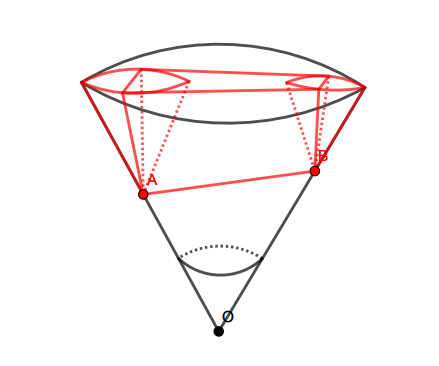
Refer to caption
Figure 1: The degenerated CC-pseudo-cone in 3\mathbb{R}^{3}

This is an example of the degenerated CC-pseudo-cone in 3\mathbb{R}^{3} and was provided by R. Schneider. In which, we place two points AA and BB on the boundary of the circular cone CC whose vertex is OO. Then the highlighted domain (in red) swept by the motion from A+CA+C to B+CB+C is a pseudo-cone, but it cannot be decomposed as Theorem 1.

Lemma 7.

Let 𝔸1,𝔸2\mathbb{A}_{1},\mathbb{A}_{2} be two CC-asymptotic sets. Then the Minkowski sum 𝔸1+𝔸2\mathbb{A}_{1}+\mathbb{A}_{2} is also a CC-asymptotic set.

Proof.

By Lemma 3, we have

𝔸1=vΩCH(v,h𝔸1(v)),𝔸2=vΩCH(v,h𝔸2(v)).\mathbb{A}_{1}=\bigcap_{v\in\Omega_{C^{\circ}}}H^{-}(v,h_{\mathbb{A}_{1}}(v)),\,\mathbb{A}_{2}=\bigcap_{v\in\Omega_{C^{\circ}}}H^{-}(v,h_{\mathbb{A}_{2}}(v)).

Clearly, 𝔸1\mathbb{A}_{1} and 𝔸2\mathbb{A}_{2} are unbounded closed convex sets contained in CC, so the Minkowski sum 𝔸1+𝔸2\mathbb{A}_{1}+\mathbb{A}_{2} is also an unbounded closed convex sets in CC. For any v𝕊n1Cv\in\mathbb{S}^{n-1}\setminus C^{\circ}, we have

sup{x+y,v|x𝔸1,y𝔸2}=sup{x,v|x𝔸1}+sup{y,v|y𝔸2}=+.\sup\{\langle x+y,v\rangle\,|\,x\in\mathbb{A}_{1},y\in\mathbb{A}_{2}\}=\sup\{\langle x,v\rangle\,|\,x\in\mathbb{A}_{1}\}+\sup\{\langle y,v\rangle\,|\,y\in\mathbb{A}_{2}\}=+\infty.

Hence, according to the closeness and convexity of 𝔸1+𝔸2\mathbb{A}_{1}+\mathbb{A}_{2}, it follows that

𝔸1+𝔸2=vΩCΩCH(v,h𝔸1+𝔸2(v)).\mathbb{A}_{1}+\mathbb{A}_{2}=\bigcap_{v\in\Omega_{C^{\circ}}\cup\partial\Omega_{C^{\circ}}}H^{-}(v,h_{\mathbb{A}_{1}+\mathbb{A}_{2}}(v)). (15)

By Corollary 1, we have h𝔸1+𝔸2(v)=h𝔸1(v)+h𝔸2(v)=0h_{\mathbb{A}_{1}+\mathbb{A}_{2}}(v)=h_{\mathbb{A}_{1}}(v)+h_{\mathbb{A}_{2}}(v)=0 for vΩCv\in\partial\Omega_{C^{\circ}}. Thus,

vΩCH(v,h𝔸1+𝔸2(v))=vΩCH(v,0)=C.\bigcap_{v\in\partial\Omega_{C^{\circ}}}H^{-}(v,h_{\mathbb{A}_{1}+\mathbb{A}_{2}}(v))=\bigcap_{v\in\partial\Omega_{C^{\circ}}}H^{-}(v,0)=C. (16)

Combining (15) with (16), one has

𝔸1+𝔸2\displaystyle\mathbb{A}_{1}+\mathbb{A}_{2} =(vΩCH(v,h𝔸1+𝔸2(v)))(vΩCH(v,0))\displaystyle=\Bigg{(}\bigcap_{v\in\Omega_{C^{\circ}}}H^{-}(v,h_{\mathbb{A}_{1}+\mathbb{A}_{2}}(v))\Bigg{)}\cap\Bigg{(}\bigcap_{v\in\partial\Omega_{C^{\circ}}}H^{-}(v,0)\Bigg{)}
=C(vΩCH(v,h𝔸1+𝔸2(v))),\displaystyle=C\cap\Bigg{(}\bigcap_{v\in\Omega_{C^{\circ}}}H^{-}(v,h_{\mathbb{A}_{1}+\mathbb{A}_{2}}(v))\Bigg{)},

which implies that conv(𝔸1+𝔸2,C)𝔸1+𝔸2\text{conv}(\mathbb{A}_{1}+\mathbb{A}_{2},C)\subset\mathbb{A}_{1}+\mathbb{A}_{2} by Definition 2. Therefore, 𝔸1+𝔸2\mathbb{A}_{1}+\mathbb{A}_{2} is a CC-compatible set. Since h𝔸1+𝔸2(v)=0h_{\mathbb{A}_{1}+\mathbb{A}_{2}}(v)=0 for all vΩCv\in\partial\Omega_{C^{\circ}}, we conclude that 𝔸1+𝔸2\mathbb{A}_{1}+\mathbb{A}_{2} is a CC-asymptotic set by Corollary 1. ∎

Corollary 2.

The Minkowski sum E+FE+F of two non-degenerated CC-pseudo-cones EE and FF is still a non-degenerated CC-pseudo-cone.

Proof.

Let z1z_{1} and z2z_{2} be the CC-starting point of EE and FF, respectively. By Theorem 5, there exists two CC-asymptotic set 𝔸1\mathbb{A}_{1} and 𝔸2\mathbb{A}_{2} such that

E=𝔸1+z1,F=𝔸2+z2.E=\mathbb{A}_{1}+z_{1},\,F=\mathbb{A}_{2}+z_{2}.

By Lemma 7, the Minkowski sum 𝔸1+𝔸2\mathbb{A}_{1}+\mathbb{A}_{2} is also a CC-asymptotic set. Noting that z1+z2Cz_{1}+z_{2}\in C and applying Theorem 5 again, the set

E+F=(𝔸1+z1)+(𝔸2+z2)=(𝔸1+𝔸2)+(z1+z2)E+F=(\mathbb{A}_{1}+z_{1})+(\mathbb{A}_{2}+z_{2})=(\mathbb{A}_{1}+\mathbb{A}_{2})+(z_{1}+z_{2})

is also a non-degenerated CC-pseudo-cone. ∎

Recently, Lemma 7 was also established by Semenov and Zhao [37]. Moreover, they also established the following results.

Lemma 8 (see [37]).

The Minkowski sum E+FE+F of two CC-pseudo-cones EE and FF is still a CC-pseudo-cone.

4 Finiteness of the asymptotic weighted co-volume

Recall that the weight function Θ:C{o}(0,)\Theta:C\setminus\{o\}\rightarrow(0,\infty) is a (q)(-q)-homogeneous continuous function with qq\in\mathbb{R}. By the compactness of the set C(1)={xC|x,𝔲=1}C(1)=\{x\in C\,|\,\langle x,\mathfrak{u}\rangle=1\}, we can define two positive constants

mΘ=minxC(1)Θ(x),MΘ=maxxC(1)Θ(x).m_{\Theta}=\min_{x\in C(1)}\Theta(x),\ \,M_{\Theta}=\max_{x\in C(1)}\Theta(x).

For any xC{o}x\in C\setminus\{o\}, since 1x,𝔲xC(1)\frac{1}{\langle x,\mathfrak{u}\rangle}x\in C(1), it follows that

mΘx,𝔲qΘ(x)MΘx,𝔲q.m_{\Theta}\langle x,\mathfrak{u}\rangle^{-q}\leqslant\Theta(x)\leqslant M_{\Theta}\langle x,\mathfrak{u}\rangle^{-q}. (17)

Let x0intEx_{0}\in\text{int}\,E and t0=x0,𝔲t_{0}=\langle x_{0},\mathfrak{u}\rangle. Then, we have x0+C=conv(x0,C)conv(E,C)=Ex_{0}+C=\text{conv}(x_{0},C)\subset\text{conv}(E,C)=E. Similar to [34], we define the sequence ti=t0+it_{i}=t_{0}+i, for ii\in\mathbb{N}, and the sequences of sets

{Ei={xE|tix,𝔲ti+1},Ei={xEi|ti<x,𝔲<ti+1},Ei¯=EC(ti+1)+{λ𝔲|1λ0},Ei¯={xEi¯|ti<x,𝔲<ti+1},Ei¯=EC(ti)+{λ𝔲| 0λ1},Ei¯={xEi¯|ti<x,𝔲<ti+1},\left\{\begin{aligned} E_{i}&=\{x\in E\,|\,t_{i}\leqslant\langle x,\mathfrak{u}\rangle\leqslant t_{i+1}\},\ \partial^{*}E_{i}=\{x\in\partial E_{i}\,|\,t_{i}<\langle x,\mathfrak{u}\rangle<t_{i+1}\},\\ \overline{E_{i}}&=E\cap C(t_{i+1})+\{\lambda\mathfrak{u}\,|\,-1\leqslant\lambda\leqslant 0\},\ \partial^{*}\overline{E_{i}}=\{x\in\partial\overline{E_{i}}\,|\,t_{i}<\langle x,\mathfrak{u}\rangle<t_{i+1}\},\\ \underline{E_{i}}&=E\cap C(t_{i})+\{\lambda\mathfrak{u}\,|\,0\leqslant\lambda\leqslant 1\},\ \partial^{*}\underline{E_{i}}=\{x\in\partial\underline{E_{i}}\,|\,t_{i}<\langle x,\mathfrak{u}\rangle<t_{i+1}\},\end{aligned}\right. (18)

where the upper cylinders Ei¯\overline{E_{i}}, lower cylinders Ei¯\underline{E_{i}}, and convex bodies EiE_{i} satisfy the relationship:

Ei¯EiEi¯.\underline{E_{i}}\subset E_{i}\subset\overline{E_{i}}. (19)

Firstly, we present the following result regrading the weighted volume of CC-pseudo-cones:

Lemma 9.

Let EE be a CC-pseudo-cone. If q>nq>n, then VΘ(E)V_{\Theta}(E) is finite; if qnq\leqslant n, then VΘ(E)V_{\Theta}(E) is infinite.

Proof.

Since Θ\Theta is continuous on C{o}C\setminus\{o\} and oEo\notin E, it follows that

EC(t0)Θ(x)𝑑n(x)<.\int_{E\cap C^{-}(t_{0})}\Theta(x)\,d\mathscr{H}^{n}(x)<\infty.

Then, the following integral can be divided as

EC(t0)Θ(x)𝑑n(x)=i=0+EiΘ(x)𝑑n(x)i=0+Ji(E).\int_{E\setminus C^{-}(t_{0})}\Theta(x)\,d\mathscr{H}^{n}(x)=\sum_{i=0}^{+\infty}\int_{E_{i}}\Theta(x)\,d\mathscr{H}^{n}(x)\triangleq\sum_{i=0}^{+\infty}J_{i}(E).

(i)(i). For q>nq>n, by (17) and (19), we have the following estimate:

Ji(E)\displaystyle J_{i}(E) EiMΘx,𝔲q𝑑n(x)\displaystyle\leqslant\int_{E_{i}}M_{\Theta}\langle x,\mathfrak{u}\rangle^{-q}\,d\mathscr{H}^{n}(x)
MΘEitiq𝑑n(x)=MΘtiqn(Ei)\displaystyle\leqslant M_{\Theta}\int_{E_{i}}t_{i}^{-q}\,d\mathscr{H}^{n}(x)=M_{\Theta}t_{i}^{-q}\mathscr{H}^{n}(E_{i})
MΘtiqn(Ei¯)=MΘtiqn1(EC(ti+1))\displaystyle\leqslant M_{\Theta}t_{i}^{-q}\mathscr{H}^{n}(\overline{E_{i}})=M_{\Theta}t_{i}^{-q}\mathscr{H}^{n-1}(E\cap C(t_{i+1}))
MΘtiqn1(C(ti+1))=MΘn1(C(1))tiq(t0+i+1)n1,\displaystyle\leqslant M_{\Theta}t_{i}^{-q}\mathscr{H}^{n-1}(C(t_{i+1}))=M_{\Theta}\mathscr{H}^{n-1}(C(1))\,t_{i}^{-q}(t_{0}+i+1)^{n-1},

which implies

limi+iqn+1Ji(E)\displaystyle\lim_{i\rightarrow+\infty}i^{q-n+1}J_{i}(E) limi+iqn+1MΘn1(C(1))tiq(t0+i+1)n1\displaystyle\leqslant\lim_{i\rightarrow+\infty}i^{q-n+1}M_{\Theta}\mathscr{H}^{n-1}(C(1))t_{i}^{-q}(t_{0}+i+1)^{n-1}
=MΘn1(C(1))limi+iq(t0+i+1)n1in1(t0+i)q\displaystyle=M_{\Theta}\mathscr{H}^{n-1}(C(1))\lim_{i\rightarrow+\infty}\frac{i^{q}(t_{0}+i+1)^{n-1}}{i^{n-1}(t_{0}+i)^{q}}
=MΘn1(C(1))<+.\displaystyle=M_{\Theta}\mathscr{H}^{n-1}(C(1))<+\infty.

According to the comparison test for pp-series, and since qn+1>1q-n+1>1, the infinite series i=0+Ji(E)\sum_{i=0}^{+\infty}J_{i}(E) is convergent, so VΘ(E)V_{\Theta}(E) is finite.
(ii)(ii). For qnq\leqslant n, as above, we have

Ji(E)\displaystyle J_{i}(E) mΘEiti+1q𝑑n(x)=mΘti+1qn(Ei)\displaystyle\geqslant m_{\Theta}\int_{E_{i}}t_{i+1}^{-q}\,d\mathscr{H}^{n}(x)=m_{\Theta}t_{i+1}^{-q}\mathscr{H}^{n}(E_{i})
mΘti+1qn(Ei¯)=mΘti+1qn1(EC(ti))\displaystyle\geqslant m_{\Theta}t_{i+1}^{-q}\mathscr{H}^{n}(\underline{E_{i}})=m_{\Theta}t_{i+1}^{-q}\mathscr{H}^{n-1}(E\cap C(t_{i}))
mΘti+1qn1((x0+C)C(ti))=mΘn1(x0+C(1))in1ti+1q\displaystyle\geqslant m_{\Theta}t_{i+1}^{-q}\mathscr{H}^{n-1}((x_{0}+C)\cap C(t_{i}))=m_{\Theta}\mathscr{H}^{n-1}(x_{0}+C(1))\,i^{n-1}t_{i+1}^{-q}
=mΘn1(C(1))in1ti+1q,\displaystyle=m_{\Theta}\mathscr{H}^{n-1}(C(1))\,i^{n-1}t_{i+1}^{-q},

which also leads to

limi+iqn+1Ji(E)\displaystyle\lim_{i\rightarrow+\infty}i^{q-n+1}J_{i}(E) mΘn1(C(1))limi+iq(t0+i+1)q=mΘn1(C(1))>0.\displaystyle\geqslant m_{\Theta}\mathscr{H}^{n-1}(C(1))\lim_{i\rightarrow+\infty}\frac{i^{q}}{(t_{0}+i+1)^{q}}=m_{\Theta}\mathscr{H}^{n-1}(C(1))>0.

Again, by the comparison test for pp-series, and since qn+11q-n+1\leqslant 1, we have i=0+Ji(E)=+\sum_{i=0}^{+\infty}J_{i}(E)=+\infty, so VΘ(E)V_{\Theta}(E) is infinite. ∎

Next, we provide the proof of a key estimate concerning the finiteness of weighted surface area measure, as discussed in [34, p. 9].

Lemma 10.

For the sets in (18), there exists a constant cc, independent of ii\in\mathbb{N}, such that

n1((Ei¯Ei)C(ti))cn2(EC(ti)).\mathscr{H}^{n-1}((\overline{E_{i}}\setminus E_{i})\cap C(t_{i}))\leqslant c\mathscr{H}^{n-2}(\partial E\cap C(t_{i})).
Proof.

Firstly, by the definitions in (18), we have

n1((Ei¯Ei)C(ti))\displaystyle\mathscr{H}^{n-1}((\overline{E_{i}}\setminus E_{i})\cap C(t_{i})) n1((Ei¯Ei)H(𝔲,ti))\displaystyle\leqslant\mathscr{H}^{n-1}((\overline{E_{i}}\setminus E_{i})\cap H(\mathfrak{u},t_{i}))
=n1(Ei¯H(𝔲,ti))n1(EiH(𝔲,ti))\displaystyle=\mathscr{H}^{n-1}(\overline{E_{i}}\cap H(\mathfrak{u},t_{i}))-\mathscr{H}^{n-1}(E_{i}\cap H(\mathfrak{u},t_{i}))
=n1(EC(ti+1))n1(EC(ti))\displaystyle=\mathscr{H}^{n-1}(E\cap C(t_{i+1}))-\mathscr{H}^{n-1}(E\cap C(t_{i}))
n1(C(ti+1))n1((x0+C)C(ti))\displaystyle\leqslant\mathscr{H}^{n-1}(C(t_{i+1}))-\mathscr{H}^{n-1}((x_{0}+C)\cap C(t_{i}))
=(t0+i+1)n1n1(C(1))in1n1(x0+C(1))\displaystyle=(t_{0}+i+1)^{n-1}\mathscr{H}^{n-1}(C(1))-i^{n-1}\mathscr{H}^{n-1}(x_{0}+C(1))
=n1(C(1))[(t0+i+1)n1in1]\displaystyle=\mathscr{H}^{n-1}(C(1))[(t_{0}+i+1)^{n-1}-i^{n-1}]
=n1(C(1))k=1n1(n1k)in1k(t0+1)k.\displaystyle=\mathscr{H}^{n-1}(C(1))\sum_{k=1}^{n-1}\dbinom{n-1}{k}i^{n-1-k}(t_{0}+1)^{k}.

Since the surface area of convex bodies increases monotonically with respect to set inclusion, we have

n2(EC(ti))n2((x0+C)C(ti))=in2n2(CC(1)),\mathscr{H}^{n-2}(\partial E\cap C(t_{i}))\geqslant\mathscr{H}^{n-2}((x_{0}+\partial C)\cap C(t_{i}))=i^{n-2}\mathscr{H}^{n-2}(\partial C\cap C(1)),

thus, we have

n1((Ei¯Ei)C(ti))n2(EC(ti))\displaystyle\frac{\mathscr{H}^{n-1}((\overline{E_{i}}\setminus E_{i})\cap C(t_{i}))}{\mathscr{H}^{n-2}(\partial E\cap C(t_{i}))} n1(C(1))n2(CC(1))k=1n1(n1k)i1k(t0+1)k\displaystyle\leqslant\frac{\mathscr{H}^{n-1}(C(1))}{\mathscr{H}^{n-2}(\partial C\cap C(1))}\sum_{k=1}^{n-1}\dbinom{n-1}{k}i^{1-k}(t_{0}+1)^{k}
n1(C(1))n2(CC(1))k=1n1(n1k)(t0+1)kc.\displaystyle\leqslant\frac{\mathscr{H}^{n-1}(C(1))}{\mathscr{H}^{n-2}(\partial C\cap C(1))}\sum_{k=1}^{n-1}\dbinom{n-1}{k}(t_{0}+1)^{k}\triangleq c.

Remark 5.

Using the above estimate, Schneider [34] proved that Sn1Θ(E,)S^{\Theta}_{n-1}(E,\cdot) is finite for any q>n1q>n-1 and every CC-pseudo-cone EE. In fact, one can also obtain the same results by using the binomial expansion and the comparison test for pp-series directly. When q<n1q<n-1, Schneider [34] provided a counterexample to show that Sn1Θ(E,ΩC)=+S^{\Theta}_{n-1}(E,\Omega_{C^{\circ}})=+\infty for some CC-pseudo-cone EE.

Counterexample 1.

For the critical case q=n1q=n-1, we provide a counterexample as follows. In the plane 2\mathbb{R}^{2}, let 𝔲=(22,22)\mathfrak{u}=(\frac{\sqrt{2}}{2},\frac{\sqrt{2}}{2}) and consider the weight function

Θ(x,y)=𝔲,(x,y)1=2x+y,(x,y)2.\Theta(x,y)=\langle\mathfrak{u},(x,y)\rangle^{-1}=\frac{\sqrt{2}}{x+y},\,(x,y)\in\mathbb{R}^{2}.

Choose a fixed cone C={(x,y)2|x0,y0}C=\{(x,y)\in\mathbb{R}^{2}\,|\,x\geqslant 0,y\geqslant 0\} and a CC-pseudo-cone

E={(x,y)C|y1x},E=\{(x,y)\in C\,|\,y\geqslant\frac{1}{x}\},

then we have

Sn1Θ(E,ΩC)\displaystyle S_{n-1}^{\Theta}(E,\Omega_{C^{\circ}}) ={(x,y)C|y=1x}Θ(x,y)𝑑s=0+2x+1x1+1x2𝑑x\displaystyle=\int_{\{(x,y)\in C\,|\,y=\frac{1}{x}\}}\Theta(x,y)\,ds=\int_{0}^{+\infty}\frac{\sqrt{2}}{x+\frac{1}{x}}\sqrt{1+\frac{1}{x^{2}}}\,dx
=20+11+x2𝑑x>21+11+x2𝑑x\displaystyle=\sqrt{2}\int_{0}^{+\infty}\frac{1}{\sqrt{1+x^{2}}}\,dx>\sqrt{2}\int_{1}^{+\infty}\frac{1}{\sqrt{1+x^{2}}}\,dx
1+1x𝑑x=+.\displaystyle\geqslant\int_{1}^{+\infty}\frac{1}{x}\,dx=+\infty.

Therefore, if qn1q\leqslant n-1, the weighted surface area measure of a CC-pseudo-cone may be infinite. However, it may also be finite, as in the case of CC-full sets.

The weighted co-volume of the CC-pseudo-cone EE can be divided into

V¯Θ(E)=(CE)𝔹nΘ(x)𝑑n(x)+(CE)𝔹nΘ(x)𝑑n(x)I0Θ(E)+IΘ(E).\overline{V}_{\Theta}(E)=\int_{(C\setminus E)\cap\,\mathbb{B}^{n}}\Theta(x)\,d\mathscr{H}^{n}(x)+\int_{(C\setminus E)\setminus\mathbb{B}^{n}}\Theta(x)\,d\mathscr{H}^{n}(x)\triangleq I^{\Theta}_{0}(E)+I^{\Theta}_{\infty}(E).

It has been proven that I0Θ(E)I^{\Theta}_{0}(E) is finite for q<nq<n and IΘ(E)I^{\Theta}_{\infty}(E) is finite for q>n1q>n-1 (see [34, Lemma 7]). Thus, V¯Θ(E)\overline{V}_{\Theta}(E) is finite for n1<q<nn-1<q<n. Here, we present some additional conclusions on the weighted co-volume.

Lemma 11.

If qnq\geqslant n, then I0Θ(E)I^{\Theta}_{0}(E) is infinite for every CC-pseudo-cone EE.

Proof.

According to (17) and the Cauchy-Schwarz inequality, we have

I0Θ(E)\displaystyle I^{\Theta}_{0}(E) =(CE)B2nΘ(x)𝑑n(x)\displaystyle=\int_{(C\setminus E)\cap B^{n}_{2}}\Theta(x)\,d\mathscr{H}^{n}(x)
mΘ(CE)B2nx,𝔲q𝑑n(x)\displaystyle\geqslant m_{\Theta}\int_{(C\setminus E)\cap B^{n}_{2}}\langle x,\mathfrak{u}\rangle^{-q}\,d\mathscr{H}^{n}(x)
mΘ(CE)B2n|x|q𝑑n(x).\displaystyle\geqslant m_{\Theta}\int_{(C\setminus E)\cap B^{n}_{2}}|x|^{-q}\,d\mathscr{H}^{n}(x).

Let r=min{1,minxE|x|}>0r=\min\{1,\min_{x\in E}|x|\}>0, then CrB2n(CE)B2nC\cap\,rB^{n}_{2}\subset(C\setminus E)\cap B^{n}_{2}. Thus,

I0Θ(E)\displaystyle I^{\Theta}_{0}(E) mΘCrB2n|x|q𝑑n(x)\displaystyle\geqslant m_{\Theta}\int_{C\cap\,rB^{n}_{2}}|x|^{-q}\,d\mathscr{H}^{n}(x)
=mΘC𝕊n10r1rqn+1𝑑r𝑑u\displaystyle=m_{\Theta}\int_{C\cap\,\mathbb{S}^{n-1}}\int_{0}^{r}\frac{1}{r^{q-n+1}}\,drdu
=mΘn1(C𝕊n1)0r1rqn+1𝑑r.\displaystyle=m_{\Theta}\mathscr{H}^{n-1}(C\cap\mathbb{S}^{n-1})\int_{0}^{r}\frac{1}{r^{q-n+1}}\,dr.

Since qn+11q-n+1\geqslant 1, we have

0r1rqn+1𝑑r=+.\int_{0}^{r}\frac{1}{r^{q-n+1}}\,dr=+\infty.

Thus, I0Θ(E)=+I^{\Theta}_{0}(E)=+\infty. ∎

Counterexample 2.

If qn1q\leqslant n-1, there is a counterexample that shows IΘ(E)I^{\Theta}_{\infty}(E) is infinite for some CC-pseudo-cone EE.

Proof.

In the plane 2\mathbb{R}^{2}, let us choose a fixed cone C={(x,y)2|x0,y0}C=\{(x,y)\in\mathbb{R}^{2}\,|\,x\geqslant 0,y\geqslant 0\} and consider the weight function

Θ(x,y)=(22,22),(x,y)q=(2x+y)q,(x,y)C,\Theta(x,y)=\big{\langle}(\frac{\sqrt{2}}{2},\frac{\sqrt{2}}{2}),(x,y)\big{\rangle}^{-q}=\Big{(}\frac{\sqrt{2}}{x+y}\Big{)}^{q},\ \,(x,y)\in C,

where 0<q10<q\leqslant 1. We construct a CC-pseudo-cone E=(1,1)+C={(x,y)2|x1,y1}E=(1,1)+C=\{(x,y)\in\mathbb{R}^{2}\,|\,x\geqslant 1,y\geqslant 1\}. For 0<q<10<q<1, we have

IΘ(E)\displaystyle I^{\Theta}_{\infty}(E) =(CE)𝔹nΘ(x,y)𝑑2(x,y)>[1,+)×[0,1](2x+y)q𝑑x𝑑y\displaystyle=\int_{(C\setminus E)\setminus\mathbb{B}^{n}}\Theta(x,y)\,d\mathscr{H}^{2}(x,y)>\int_{[1,+\infty)\times[0,1]}\Big{(}\frac{\sqrt{2}}{x+y}\Big{)}^{q}\,dxdy
=2q21+(011(x+y)q𝑑y)𝑑x=2q21q1+((1+x)1qx1q)𝑑x.\displaystyle=2^{\frac{q}{2}}\int_{1}^{+\infty}\bigg{(}\int_{0}^{1}\frac{1}{(x+y)^{q}}\,dy\bigg{)}\,dx=\frac{2^{\frac{q}{2}}}{1-q}\int_{1}^{+\infty}\big{(}(1+x)^{1-q}-x^{1-q}\big{)}\,dx.

Since

limx+(1+1x)1q11x=1q(0,1),\lim_{x\rightarrow+\infty}\frac{(1+\frac{1}{x})^{1-q}-1}{\frac{1}{x}}=1-q\in(0,1),

there exists N>1N>1 such that

(1+x)1qx1q=x1q((1+1x)1q1)1q2xq(1+x)^{1-q}-x^{1-q}=x^{1-q}\Big{(}(1+\frac{1}{x})^{1-q}-1\Big{)}\geqslant\frac{1-q}{2}\,x^{-q}

for all x>Nx>N. Thus,

IΘ(E)\displaystyle I^{\Theta}_{\infty}(E) =2q21q1+((1+x)1qx1q)𝑑x\displaystyle=\frac{2^{\frac{q}{2}}}{1-q}\int_{1}^{+\infty}\big{(}(1+x)^{1-q}-x^{1-q}\big{)}\,dx
2q21q(1N((1+x)1qx1q)𝑑x+1q2N+1xq𝑑x)\displaystyle\geqslant\frac{2^{\frac{q}{2}}}{1-q}\bigg{(}\int_{1}^{N}\big{(}(1+x)^{1-q}-x^{1-q}\big{)}\,dx+\frac{1-q}{2}\int_{N}^{+\infty}\frac{1}{x^{q}}\,dx\bigg{)}
=+.\displaystyle=+\infty.

For q=1q=1, since

limx+log(1+1x)1x=1,\lim_{x\rightarrow+\infty}\frac{\log(1+\frac{1}{x})}{\frac{1}{x}}=1,

there exists a constant N>1N>1 such that log(1+1x)>12x\log(1+\frac{1}{x})>\frac{1}{2x} for all x>Nx>N. Thus, we have

IΘ(E)\displaystyle I^{\Theta}_{\infty}(E) >21+(011x+y𝑑y)𝑑x=21+log(1+1x)𝑑x\displaystyle>\sqrt{2}\int_{1}^{+\infty}\bigg{(}\int_{0}^{1}\frac{1}{x+y}\,dy\bigg{)}\,dx=\sqrt{2}\int_{1}^{+\infty}\log(1+\frac{1}{x})\,dx
2(1Nlog(1+1x)𝑑x+N+12x𝑑x)=+.\displaystyle\geqslant\sqrt{2}\bigg{(}\int_{1}^{N}\log(1+\frac{1}{x})\,dx+\int_{N}^{+\infty}\frac{1}{2x}\,dx\bigg{)}=+\infty.

Therefore, if qn1q\leqslant n-1, then IΘ(E)I^{\Theta}_{\infty}(E) may be infinite. However, it may also be finite. ∎

Recall the pp-improper integral over infinite interval:

1+1xpdx={finite value,p>1,+,p1,\int_{1}^{+\infty}\frac{1}{x^{p}}\,dx=\left\{\begin{aligned} &\text{finite value},\ &p>1,\\ &+\infty,\ &p\leqslant 1,\end{aligned}\right.

and the pp-improper integral with singularities:

011xpdx={+,p1,finite value,p<1.\int_{0}^{1}\frac{1}{x^{p}}\,dx=\left\{\begin{aligned} &+\infty,\ &p\geqslant 1,\\ &\text{finite value},\ &p<1.\end{aligned}\right.

From the above discussion, it is clear that the weighted volume VΘ(E)V_{\Theta}(E) of a CC-pseudo-cone EE is the natural nn-dimensional generalization of the pp-improper integral over infinite interval, and the integral I0Θ(E)I^{\Theta}_{0}(E) is the natural nn-dimensional generalization of the pp-improper integral with singularities. However, neither VΘ(E)V_{\Theta}(E) nor I0Θ(E)I^{\Theta}_{0}(E) effectively captures the relative information about EE. Furthermore, the weighted co-volume V¯Θ(E)\overline{V}_{\Theta}(E) calculates some invalid volumes of EE form the perspective of the CC-starting point of EE. Therefore, we will focus on studying the asymptotic behavior of the weighted co-volume of EE.

Definition 5.

Let zz be the CC-starting point of CC-pseudo-cone EE, i.e., EE can be decomposed into the sum of a CC-asymptotic set 𝔸\mathbb{A} and the CC-starting point zz, then we define the asymptotic weighted co-volume of EE by

TΘ(E)=TΘ(𝔸,z)=VΘ((z+C)E)=(z+C)EΘ(x)𝑑n(x).T_{\Theta}(E)=T_{\Theta}(\mathbb{A},z)=V_{\Theta}((z+C)\setminus E)=\int_{(z+C)\setminus E}\Theta(x)\,d\mathscr{H}^{n}(x).
Remark 6.

Here we consider this asymptotic weighted co-volume TΘ(E)T_{\Theta}(E) as a functional of two variables. Thus, if we fix a CC-asymptotic set 𝔸\mathbb{A}, then TΘ(E)=TΘ(𝔸,)T_{\Theta}(E)=T_{\Theta}(\mathbb{A},\cdot) is precisely a generalized function on the cone CC.

It is evident that the weighted volume VΘ(E)V_{\Theta}(E) of a CC-pseudo-cone EE serves the nn-dimensional generalization of the pp-improper integral over infinite interval. However, the nn-dimensional generalization of the pp-improper integral with singularities is more intricate, involving both the weighted co-volume V¯Θ(E)\overline{V}_{\Theta}(E) and the asymptotic weighted co-volume TΘ(𝔸,z)T_{\Theta}(\mathbb{A},z). Moreover, the properties of the asymptotic weighted co-volume are superior to those of the weighted co-volume.

Lemma 12.

Let EE be a CC-asymptotic set and q>n1q>n-1. If zoz\neq o, TΘ(E,z)T_{\Theta}(E,z) is finite. If z=oz=o, the following holds:

TΘ(E,o)={finite,n1<q<n,+,qn.T_{\Theta}(E,o)=\left\{\begin{aligned} &\text{finite},\ n-1<q<n,\\ &+\infty,\ q\geqslant n.\end{aligned}\right.

Thus, the origin oo is the unique singularity of TΘ(E,)T_{\Theta}(E,\cdot) for qnq\geqslant n.

Proof.

According to the definition of the asymptotic weighted co-volume, we have

TΘ(E,z)\displaystyle T_{\Theta}(E,z) =((z+C)E)C(t0)Θ(x)𝑑n(x)+t0+((z+C)E)C(t)Θ(x)𝑑n1(x)𝑑t\displaystyle=\int_{((z+C)\setminus E)\cap C^{-}(t_{0})}\Theta(x)\,d\mathscr{H}^{n}(x)+\int_{t_{0}}^{+\infty}\int_{((z+C)\setminus E)\cap C(t)}\Theta(x)\,d\mathscr{H}^{n-1}(x)\,dt
J1~(E)+J2~(E).\displaystyle\triangleq\widetilde{J_{1}}(E)+\widetilde{J_{2}}(E).

(i)(i) If zoz\neq o, since Θ\Theta is continuous on C{o}C\setminus\{o\} and ((z+C)E)C(t0)C{o}((z+C)\setminus E)\cap C^{-}(t_{0})\subset C\setminus\{o\} is compact, the integral J1~(E)\widetilde{J_{1}}(E) is finite. Similar to Lemma 7 in [34], using (17), we obtain

J2~(E)\displaystyle\widetilde{J_{2}}(E) t0+((z+C)E)C(t)MΘtq𝑑n1(x)𝑑t\displaystyle\leqslant\int_{t_{0}}^{+\infty}\int_{((z+C)\setminus E)\cap C(t)}M_{\Theta}t^{-q}\,d\mathscr{H}^{n-1}(x)\,dt
=MΘt0+tq(n1((z+C)C(t))n1(EC(t)))𝑑t\displaystyle=M_{\Theta}\int_{t_{0}}^{+\infty}t^{-q}\big{(}\mathscr{H}^{n-1}((z+C)\cap C(t))-\mathscr{H}^{n-1}(E\cap C(t))\big{)}\,dt
MΘt0+tq((tz,𝔲)n1n1(CC(1))(tt0)n1n1(CC(1)))𝑑t\displaystyle\leqslant M_{\Theta}\int_{t_{0}}^{+\infty}t^{-q}\big{(}(t-\langle z,\mathfrak{u}\rangle)^{n-1}\mathscr{H}^{n-1}(C\cap C(1))-(t-t_{0})^{n-1}\mathscr{H}^{n-1}(C\cap C(1))\big{)}\,dt
=MΘn1(CC(1))t0+tq((tz,𝔲)n1(tt0)n1)𝑑t.\displaystyle=M_{\Theta}\mathscr{H}^{n-1}(C\cap C(1))\int_{t_{0}}^{+\infty}t^{-q}\big{(}(t-\langle z,\mathfrak{u}\rangle)^{n-1}-(t-t_{0})^{n-1}\big{)}\,dt.

Next, using the binomial expansion:

t0+tq((tz,𝔲)n1(tt0)n1)𝑑t=i=1n1(n1i)((z,𝔲)i(t0)i)t0+1tq+1+in𝑑t.\displaystyle\int_{t_{0}}^{+\infty}\!\!\!\!\!t^{-q}\big{(}(t-\langle z,\mathfrak{u}\rangle)^{n-1}-(t-t_{0})^{n-1}\big{)}\,dt\!=\!\sum_{i=1}^{n-1}\dbinom{n-1}{i}\big{(}(-\langle z,\mathfrak{u}\rangle)^{i}-(-t_{0})^{i}\big{)}\int_{t_{0}}^{+\infty}\!\!\!\!\!\frac{1}{t^{q+1+i-n}}\,dt.

Since q>n1q>n-1, we have q+1+in>i1q+1+i-n>i\geqslant 1 for i=1,,n1i=1,\cdots,n-1, which implies that

t0+1tq+1+in𝑑t<+.\int_{t_{0}}^{+\infty}\frac{1}{t^{q+1+i-n}}\,dt<+\infty.

Thus, TΘ(E,z)T_{\Theta}(E,z) is finite.
(ii)(ii) If z=oz=o, similar to [34, p. 13] and Lemma 11, for n1<q<nn-1<q<n we have

J1~(E)\displaystyle\widetilde{J_{1}}(E) =(CE)C(t0)Θ(x)𝑑n(x)MΘcqB2n(R)|x|q𝑑n(x)\displaystyle=\int_{(C\setminus E)\cap C^{-}(t_{0})}\Theta(x)\,d\mathscr{H}^{n}(x)\leqslant M_{\Theta}c^{-q}\int_{B^{n}_{2}(R)}|x|^{-q}\,d\mathscr{H}^{n}(x)
=nωnMΘcq0R1rq+1n𝑑r<+.\displaystyle=n\omega_{n}M_{\Theta}c^{-q}\int_{0}^{R}\frac{1}{r^{q+1-n}}\,dr<+\infty.

For qnq\geqslant n, we have

J1~(E)=(CE)C(t0)Θ(x)𝑑n(x)mΘ(CE)C(t0)|x|q𝑑n(x).\widetilde{J_{1}}(E)=\int_{(C\setminus E)\cap C^{-}(t_{0})}\Theta(x)\,d\mathscr{H}^{n}(x)\geqslant m_{\Theta}\int_{(C\setminus E)\cap C^{-}(t_{0})}|x|^{-q}\,d\mathscr{H}^{n}(x).

Let r=min{t0,minxE|x|}>0r=\min\{t_{0},\min_{x\in E}|x|\}>0, then CrB2n(CE)C(t0)C\cap\,rB^{n}_{2}\subset(C\setminus E)\cap C^{-}(t_{0}). Thus,

J1~(E)mΘCrB2n|x|q𝑑n(x)=mΘn1(C𝕊n1)0r1rqn+1𝑑r=+.\widetilde{J_{1}}(E)\geqslant m_{\Theta}\int_{C\cap\,rB^{n}_{2}}|x|^{-q}\,d\mathscr{H}^{n}(x)=m_{\Theta}\mathscr{H}^{n-1}(C\cap\mathbb{S}^{n-1})\int_{0}^{r}\frac{1}{r^{q-n+1}}\,dr=+\infty.

It is easy to check that J2~(E)<+\widetilde{J_{2}}(E)<+\infty for z=oz=o. Therefore,

TΘ(E,o)={finite,n1<q<n,infinite,qn.T_{\Theta}(E,o)=\left\{\begin{aligned} &\text{finite},\ &n-1<q<n,\\ &\text{infinite},\ &q\geqslant n.\end{aligned}\right.

Moreover, it is not hard to prove that TΘ(E,z)T_{\Theta}(E,z) is continuous, that is, TΘ(Ei,zi)TΘ(E,z)T_{\Theta}(E_{i},z_{i})\rightarrow T_{\Theta}(E,z) as (Ei,zi)(E,z)(E_{i},z_{i})\rightarrow(E,z), similarly to [34, p. 14]. ∎

Counterexample 3.

Let qn1q\leqslant n-1 and zoz\neq o. Then there exists some CC-asymptotic set EE such that TΘ(E,z)=+T_{\Theta}(E,z)=+\infty.

Proof.

Choose a fixed cone C={(x,y)2|x0,y0}C=\{(x,y)\in\mathbb{R}^{2}\,|\,x\geqslant 0,y\geqslant 0\} and consider the weight function

Θ(x,y)=(2x+y)q,(x,y)C,\Theta(x,y)=\Big{(}\frac{\sqrt{2}}{x+y}\Big{)}^{q},\,(x,y)\in C,

where 0<q10<q\leqslant 1. Let E={(x,y)C|y1x}E=\{(x,y)\in C\,|\,y\geqslant\frac{1}{x}\} be a CC-asymptotic set, and choose a CC-starting point z=(1,1)z=(1,1). For 0<q<10<q<1, we have

TΘ(E,z)\displaystyle T_{\Theta}(E,z) =(z+C)EΘ(x,y)𝑑2(x,y)>{(x,y)C|x2,1y1+1x}(2x+y)q𝑑x𝑑y\displaystyle=\int_{(z+C)\setminus E}\Theta(x,y)\,d\mathscr{H}^{2}(x,y)>\int_{\{(x,y)\in C\,|\,x\geqslant 2,1\leqslant y\leqslant 1+\frac{1}{x}\}}\Big{(}\frac{\sqrt{2}}{x+y}\Big{)}^{q}\,dxdy
=2q22+(11+x1(x+y)q𝑑y)𝑑x=2q21q2+((1+2x)1q(1+x)1q)𝑑x.\displaystyle=2^{\frac{q}{2}}\int_{2}^{+\infty}\bigg{(}\int_{1}^{1+x}\frac{1}{(x+y)^{q}}\,dy\bigg{)}\,dx=\frac{2^{\frac{q}{2}}}{1-q}\int_{2}^{+\infty}\big{(}(1+2x)^{1-q}-(1+x)^{1-q}\big{)}\,dx.

According to the limit

limx+(1+x1+x)1q1=21q1(0,1),\lim_{x\rightarrow+\infty}(1+\frac{x}{1+x})^{1-q}-1=2^{1-q}-1\in(0,1),

there exists N>1N>1 such that

(1+2x)1q(1+x)1q=(1+x)1q((1+x1+x)1q1)>21q12x1q(1+2x)^{1-q}-(1+x)^{1-q}=(1+x)^{1-q}\Big{(}(1+\frac{x}{1+x})^{1-q}-1\Big{)}>\frac{2^{1-q}-1}{2}\,x^{1-q}

for all x>Nx>N. Thus,

TΘ(E,z)\displaystyle T_{\Theta}(E,z) >2q21q2+((1+2x)1q(1+x)1q)𝑑x\displaystyle>\frac{2^{\frac{q}{2}}}{1-q}\int_{2}^{+\infty}\big{(}(1+2x)^{1-q}-(1+x)^{1-q}\big{)}\,dx
2q21q(2N((1+2x)1q(1+x)1q)𝑑x+21q12N+x1q𝑑x)\displaystyle\geqslant\frac{2^{\frac{q}{2}}}{1-q}\bigg{(}\int_{2}^{N}\big{(}(1+2x)^{1-q}-(1+x)^{1-q}\big{)}\,dx+\frac{2^{1-q}-1}{2}\int_{N}^{+\infty}x^{1-q}\,dx\bigg{)}
=+.\displaystyle=+\infty.

For q=1q=1, due to

limx+log(1+x1+x)=log2,\lim_{x\rightarrow+\infty}\log(1+\frac{x}{1+x})=\log 2,

there exists a constant N>1N>1 such that log(1+x1+x)>12log2\log(1+\frac{x}{1+x})>\frac{1}{2}\log 2 for all x>Nx>N. Thus,

TΘ(E,z)\displaystyle T_{\Theta}(E,z) >22+(11+x1x+y𝑑y)𝑑x=22+log(1+x1+x)𝑑x\displaystyle>\sqrt{2}\int_{2}^{+\infty}\bigg{(}\int_{1}^{1+x}\frac{1}{x+y}\,dy\bigg{)}\,dx=\sqrt{2}\int_{2}^{+\infty}\log(1+\frac{x}{1+x})\,dx
2(2Nlog(1+x1+x)𝑑x+12log2N+𝑑x)=+.\displaystyle\geqslant\sqrt{2}\bigg{(}\int_{2}^{N}\log(1+\frac{x}{1+x})\,dx+\frac{1}{2}\log 2\int_{N}^{+\infty}dx\bigg{)}=+\infty.

Therefore, if qn1q\leqslant n-1, the asymptotic weighted co-volume may be infinite, but it can also be finite. ∎

Proof of Theorem 2.

Let EE be a CC-pseudo-cone and let 𝔸\mathbb{A} be a CC-asymptotic set with zoz\neq o. According to Lemma 11, the weighted co-volume V¯Θ(E)\overline{V}_{\Theta}(E) is infinite for qnq\geqslant n; as stated in Remark 2, V¯Θ(E)\overline{V}_{\Theta}(E) can be either finite or infinite for 0<qn10<q\leqslant n-1. The behavior of TΘ(𝔸,o)T_{\Theta}(\mathbb{A},o) is same as V¯Θ(E)\overline{V}_{\Theta}(E). By Remark 5, the weighted surface area measure Sn1Θ(E,ΩC)S_{n-1}^{\Theta}(E,\Omega_{C^{\circ}}) can also be finite or infinite for 0qn10\leqslant q\leqslant n-1. From Lemma 9, the weighted volume VΘ(E)V_{\Theta}(E) is finite for q>nq>n and infinite for 0<qn0<q\leqslant n. According to Lemma 12 and Remark 3, TΘ(𝔸,z)T_{\Theta}(\mathbb{A},z) is finite for q>n1q>n-1, but it may be finite or infinite for 0<qn10<q\leqslant n-1. Finally, combining these results with those in [34], we can derive Theorem 2, which summarizes the behavior of the weighted co-volume, surface area measure, and asymptotic weighted co-volume.

condition measure Sn1Θ(E,)S_{n-1}^{\Theta}(E,\cdot) VΘ(E)V_{\Theta}(E) V¯Θ(E)\overline{V}_{\Theta}(E) TΘ(𝔸,o)T_{\Theta}(\mathbb{A},o) TΘ(𝔸,z)T_{\Theta}(\mathbb{A},z)
q>nq>n finite finite ++\infty ++\infty finite
q=nq=n finite ++\infty ++\infty ++\infty finite
n1<q<nn-1<q<n finite ++\infty finite finite finite
0<qn10<q\leqslant n-1 finite or ++\infty ++\infty finite or ++\infty finite or ++\infty finite or ++\infty

In the table above, the blue color indicates that there is some useful and interesting information. ∎

5 Integral formulas and convolution formulas

In Sections 3 and 4, we discussed several notable properties of the asymptotic CC-pseudo-cone. Based on these properties, we can explore the relationships between Sn1Θ(E,)S^{\Theta}_{n-1}(E,\cdot), V¯Θ(E)\overline{V}_{\Theta}(E), and TΘ(E)T_{\Theta}(E). Firstly, we present the following results.

Lemma 13.

Let EE be a CC-pseudo-cone and 0q<n0\leqslant q<n. Then, there exist integral representations of the weighted co-volume of EE as follows:

V¯Θ(E)\displaystyle\overline{V}_{\Theta}(E) =1nqΩCeΘ(u)ρEnq(u)𝑑u,\displaystyle=\frac{1}{n-q}\int_{\Omega_{C}^{e}}\Theta(u)\rho^{n-q}_{E}(u)\,du, (20)
V¯Θ(E)\displaystyle\overline{V}_{\Theta}(E) =1nqΩCeh¯E(v)𝑑Sn1Θ(E,v).\displaystyle=\frac{1}{n-q}\int_{\Omega_{C^{\circ}}^{e}}\overline{h}_{E}(v)\,dS^{\Theta}_{n-1}(E,v). (21)
Proof.

By using polar coordinates and the Newton-Leibniz formula for integrals, we have

V¯Θ(E)=ΩCe0ρE(u)Θ(ru)rn1𝑑r𝑑u=1nqΩCeΘ(u)ρEnq(u)𝑑u.\overline{V}_{\Theta}(E)=\int_{\Omega_{C}^{e}}\int_{0}^{\rho_{E}(u)}\Theta(ru)r^{n-1}\,drdu=\frac{1}{n-q}\int_{\Omega_{C}^{e}}\Theta(u)\rho^{n-q}_{E}(u)\,du.

Applying the co-area formula (6), we obtain

V¯Θ(E)\displaystyle\overline{V}_{\Theta}(E) =1nqΩCeΘ(u)ρEq(u)h¯E(αE(u))ρEn(u)h¯E(αE(u))𝑑μ𝕊n1(u)\displaystyle=\frac{1}{n-q}\int_{\Omega_{C}^{e}}\Theta(u)\rho^{-q}_{E}(u)\overline{h}_{E}(\alpha_{E}(u))\frac{\rho_{E}^{n}(u)}{\overline{h}_{E}(\alpha_{E}(u))}\,d\mu_{\mathbb{S}^{n-1}}(u)
=1nqeEΘ(x|x|)|x|qh¯E(νE(x))𝑑n1(x)\displaystyle=\frac{1}{n-q}\int_{\partial_{e}E}\Theta\left(\frac{x}{|x|}\right)|x|^{-q}\overline{h}_{E}(\nu_{E}(x))\,d\mathscr{H}^{n-1}(x)
=1nqeEh¯E(νE(x))Θ(x)𝑑n1(x),\displaystyle=\frac{1}{n-q}\int_{\partial_{e}E}\overline{h}_{E}(\nu_{E}(x))\Theta(x)\,d\mathscr{H}^{n-1}(x),

where h¯E(αE(u))=h¯E(νE(x))>0\overline{h}_{E}(\alpha_{E}(u))=\overline{h}_{E}(\nu_{E}(x))>0. By the push-forward formula (5), we conclude that

eEh¯E(νE(x))Θ(x)𝑑n1(x)=ΩCeh¯E(v)𝑑Sn1Θ(E,v).\int_{\partial_{e}E}\overline{h}_{E}(\nu_{E}(x))\Theta(x)\,d\mathscr{H}^{n-1}(x)=\int_{\Omega_{C^{\circ}}^{e}}\overline{h}_{E}(v)\,dS^{\Theta}_{n-1}(E,v).

Remark 7.

The integral formula analogous to (21) for the volume functional in the classical case can be established using approximations of convex polytopes (see e.g., [28, p. 275-276]). The study of the push-forward measure of the radial Gauss image was first undertaken by [16], utilizing the Gauss-Green formula for finite perimeter sets and various approximation techniques. In fact, the co-area formula of Federer [13] serves as a more powerful tool for these problems (see [28, chapter. 4] and [18, p. 170]). Generally, the volume formulas for general measures with continuous density have also been derived using the co-area formula, as demonstrated in [20]. In the case of CC-close sets, Schneider [30] utilized the volume formula for convex bodies in conjunction with approximation methods. Here, we also present a general version of the volume formula (21) utilizing the co-area formula.

Lemma 14.

Suppose q>n1q>n-1. Let EE be a CC-pseudo-cone with its decomposition E=z+𝔸E=z+\mathbb{A} for the CC-asymptotic set 𝔸\mathbb{A} and the starting point zoz\neq o. If qnq\neq n, we have

TΘ(𝔸,z)\displaystyle T_{\Theta}(\mathbb{A},z) =1nqΩCeh¯E(v)𝑑Sn1Θ(E,v)\displaystyle=\frac{1}{n-q}\int_{\Omega_{C^{\circ}}^{e}}\overline{h}_{E}(v)\,dS_{n-1}^{\Theta}(E,v) (22)
+1nqΩCz,v𝑑Sn1Θ(z+C,v).\displaystyle\quad+\frac{1}{n-q}\int_{\partial\Omega_{C^{\circ}}}\langle z,v\rangle\,dS_{n-1}^{\Theta}(z+C,v).

If q=nq=n, we have

TΘ(𝔸,z)\displaystyle T_{\Theta}(\mathbb{A},z) =eEΘ(x)h¯E(νE(x))log|x|dn1(x)\displaystyle=\int_{\partial_{e}E}\Theta(x)\overline{h}_{E}(\nu_{E}(x))\log|x|\,d\mathscr{H}^{n-1}(x) (23)
+z+CΘ(x)z,νz+C(x)log|x|dn1(x).\displaystyle\quad+\int_{z+\partial C}\Theta(x)\langle z,\nu_{z+C}(x)\rangle\log|x|\,d\mathscr{H}^{n-1}(x).
Proof.

If nq>n1n\neq q>n-1, since zoz\neq o, we have ΩCe=ΩC\Omega_{C}^{e}=\Omega_{C} and eE=E\partial_{e}E=\partial E. Thus,

TΘ(𝔸,z)\displaystyle T_{\Theta}(\mathbb{A},z) =(z+C)EΘ(x)𝑑n(x)=ΩCeρz+C(u)ρE(u)Θ(ru)rn1𝑑r𝑑u\displaystyle=\int_{(z+C)\setminus E}\Theta(x)\,d\mathscr{H}^{n}(x)=\int_{\Omega_{C}^{e}}\int_{\rho_{z+C}(u)}^{\rho_{E}(u)}\Theta(ru)r^{n-1}\,drdu
=ΩCeΘ(u)ρz+C(u)ρE(u)rn1q𝑑r𝑑u=1nqΩCeΘ(u)(ρEnq(u)ρz+Cnq(u))𝑑u\displaystyle=\int_{\Omega_{C}^{e}}\Theta(u)\int_{\rho_{z+C}(u)}^{\rho_{E}(u)}r^{n-1-q}\,drdu=\frac{1}{n-q}\int_{\Omega_{C}^{e}}\Theta(u)(\rho^{n-q}_{E}(u)-\rho^{n-q}_{z+C}(u))\,du
=1nqΩCeΘ(u)ρEnq(u)𝑑u1nqΩCΘ(u)ρz+Cnq(u)𝑑u\displaystyle=\frac{1}{n-q}\int_{\Omega_{C}^{e}}\Theta(u)\rho^{n-q}_{E}(u)\,du-\frac{1}{n-q}\int_{\Omega_{C}}\Theta(u)\rho^{n-q}_{z+C}(u)\,du
=1nqeEΘ(x)h¯E(νE(x))𝑑n1(x)\displaystyle=\frac{1}{n-q}\int_{\partial_{e}E}\Theta(x)\overline{h}_{E}(\nu_{E}(x))\,d\mathscr{H}^{n-1}(x)
1nqz+CΘ(x)h¯z+C(νz+C(x))𝑑n1(x)\displaystyle\quad-\frac{1}{n-q}\int_{z+\partial C}\Theta(x)\overline{h}_{z+C}(\nu_{z+C}(x))\,d\mathscr{H}^{n-1}(x)
=1nqΩCeh¯E(v)𝑑Sn1Θ(E,v)+1nqΩCz,v𝑑Sn1Θ(z+C,v).\displaystyle=\frac{1}{n-q}\int_{\Omega_{C^{\circ}}^{e}}\overline{h}_{E}(v)\,dS_{n-1}^{\Theta}(E,v)+\frac{1}{n-q}\int_{\partial\Omega_{C^{\circ}}}\langle z,v\rangle\,dS_{n-1}^{\Theta}(z+C,v).

If q=nq=n, we have

TΘ(𝔸,z)\displaystyle T_{\Theta}(\mathbb{A},z) =ΩCeΘ(u)ρz+C(u)ρE(u)1r𝑑r𝑑u\displaystyle=\int_{\Omega_{C}^{e}}\Theta(u)\int_{\rho_{z+C}(u)}^{\rho_{E}(u)}\frac{1}{r}\,drdu
=ΩCeΘ(u)(logρE(u)logρz+C(u))𝑑u\displaystyle=\int_{\Omega_{C}^{e}}\Theta(u)(\log\rho_{E}(u)-\log\rho_{z+C}(u))\,du
=ΩCeΘ(u)logρE(u)𝑑uΩCΘ(u)logρz+C(u)𝑑u\displaystyle=\int_{\Omega_{C}^{e}}\Theta(u)\log\rho_{E}(u)\,du-\int_{\Omega_{C}}\Theta(u)\log\rho_{z+C}(u)\,du
=eEΘ(x)h¯E(νE(x))log|x|dn1(x)\displaystyle=\int_{\partial_{e}E}\Theta(x)\overline{h}_{E}(\nu_{E}(x))\log|x|\,d\mathscr{H}^{n-1}(x)
+z+CΘ(x)z,νz+C(x)log|x|dn1(x).\displaystyle\quad+\int_{z+\partial C}\Theta(x)\langle z,\nu_{z+C}(x)\rangle\log|x|\,d\mathscr{H}^{n-1}(x).

According to the definition of the rr-th dual volume V~r()\widetilde{V}_{r}(\cdot) given in [22], the formula (20) implies that V~r()\widetilde{V}_{r}(\cdot) is finite, as follows.

Corollary 3.

For any r(,0)(0,1)r\in(-\infty,0)\cup(0,1), the rr-th dual volume V~r(E)\widetilde{V}_{r}(E) is finite for every CC-pseudo-cone EE.

Proof.

Let r<0r<0. Then we have

V~r(E)=1nΩCeρEr(u)𝑑u1n(minuΩCeρE(u))rΩCe𝑑u<+.\widetilde{V}_{r}(E)=\frac{1}{n}\int_{\Omega_{C}^{e}}\rho^{r}_{E}(u)\,du\leqslant\frac{1}{n}\big{(}\min_{u\in\Omega_{C}^{e}}\rho_{E}(u)\big{)}^{r}\int_{\Omega_{C}^{e}}du<+\infty.

Now, let r(0,1)r\in(0,1) with r=nqr=n-q, so q(n1,n)q\in(n-1,n). By the estimate (17), the formula (20), and the Cauchy-Schwarz inequality, we have

V¯Θ(E)\displaystyle\overline{V}_{\Theta}(E) =1nqΩCeΘ(u)ρEnq(u)𝑑u\displaystyle=\frac{1}{n-q}\int_{\Omega_{C}^{e}}\Theta(u)\rho^{n-q}_{E}(u)\,du
mΘnqΩCeu,𝔲qρEnq(u)𝑑u\displaystyle\geqslant\frac{m_{\Theta}}{n-q}\int_{\Omega_{C}^{e}}\langle u,\mathfrak{u}\rangle^{-q}\rho^{n-q}_{E}(u)\,du
mΘnqΩCeρEnq(u)𝑑u.\displaystyle\geqslant\frac{m_{\Theta}}{n-q}\int_{\Omega_{C}^{e}}\rho^{n-q}_{E}(u)\,du.

Thus, according to the finiteness of the weighted co-volume, we have

V~r(E)=V~nq(E)=1nΩCeρEnq(u)𝑑unqnmΘV¯Θ(E)<+.\widetilde{V}_{r}(E)=\widetilde{V}_{n-q}(E)=\frac{1}{n}\int_{\Omega_{C}^{e}}\rho^{n-q}_{E}(u)\,du\leqslant\frac{n-q}{n\,m_{\Theta}}\overline{V}_{\Theta}(E)<+\infty.

Lemma 15.

Let EE be a CC-pseudo-cone with its decomposition E=z+𝔸E=z+\mathbb{A} for the CC-asymptotic set 𝔸\mathbb{A} and the starting point zoz\neq o. If q>0q>0, we have the following convolution formula:

TΘ(𝔸,z)+VΘ(E)=𝝌CΘ(z).T_{\Theta}(\mathbb{A},z)+V_{\Theta}(E)=\boldsymbol{\chi}_{-C}\ast\Theta\,(z). (24)

In particular, if q>nq>n, we have

TΘ(𝔸,z)=𝝌CΘ(z)VΘ(z+𝔸),zC.T_{\Theta}(\mathbb{A},z)=\boldsymbol{\chi}_{-C}\ast\Theta\,(z)-V_{\Theta}(z+\mathbb{A}),\,z\in C. (25)
Proof.

Suppose q>nq>n. For zoz\neq o, both VΘ(E)V_{\Theta}(E) and TΘ(𝔸,z)T_{\Theta}(\mathbb{A},z) are finite. Noting that

𝝌z+C(x)=𝝌C(xz)=𝝌C(zx),xn,\boldsymbol{\chi}_{z+C}(x)=\boldsymbol{\chi}_{C}(x-z)=\boldsymbol{\chi}_{-C}(z-x),\,x\in\mathbb{R}^{n},

we have

TΘ(𝔸,z)\displaystyle T_{\Theta}(\mathbb{A},z) =n𝝌(z+C)E(x)Θ(x)𝑑n(x)\displaystyle=\int_{\mathbb{R}^{n}}\boldsymbol{\chi}_{(z+C)\setminus E}(x)\,\Theta(x)\,d\mathscr{H}^{n}(x)
=n(𝝌z+C(x)𝝌E(x))Θ(x)𝑑n(x)\displaystyle=\int_{\mathbb{R}^{n}}\big{(}\boldsymbol{\chi}_{z+C}(x)-\boldsymbol{\chi}_{E}(x)\big{)}\Theta(x)\,d\mathscr{H}^{n}(x)
=n𝝌z+C(x)Θ(x)𝑑n(x)n𝝌E(x)Θ(x)𝑑n(x)\displaystyle=\int_{\mathbb{R}^{n}}\boldsymbol{\chi}_{z+C}(x)\Theta(x)\,d\mathscr{H}^{n}(x)-\int_{\mathbb{R}^{n}}\boldsymbol{\chi}_{E}(x)\Theta(x)\,d\mathscr{H}^{n}(x)
=n𝝌C(zx)Θ(x)𝑑n(x)EΘ(x)𝑑n(x)\displaystyle=\int_{\mathbb{R}^{n}}\boldsymbol{\chi}_{-C}(z-x)\Theta(x)\,d\mathscr{H}^{n}(x)-\int_{E}\Theta(x)\,d\mathscr{H}^{n}(x)
=𝝌CΘ(z)VΘ(E),\displaystyle=\boldsymbol{\chi}_{-C}\ast\Theta\,(z)-V_{\Theta}(E),

where the weight function Θ\Theta can be extended to the whole space n\mathbb{R}^{n}, making the convolution 𝝌CΘ\boldsymbol{\chi}_{-C}\ast\Theta well-defined.

For z=oz=o, we have TΘ(𝔸,o)=+T_{\Theta}(\mathbb{A},o)=+\infty and

𝝌CΘ(o)=CΘ(x)𝑑n(x)>CB2nΘ(x)𝑑n(x)=+.\boldsymbol{\chi}_{-C}\ast\Theta\,(o)=\int_{C}\Theta(x)\,d\mathscr{H}^{n}(x)>\int_{C\cap B^{n}_{2}}\Theta(x)\,d\mathscr{H}^{n}(x)=+\infty.

Thus, (25) holds. Since VΘ(E)V_{\Theta}(E) is finite, (24) also holds for q>nq>n.

Now, suppose qnq\leqslant n. In this case, VΘ(E)=+V_{\Theta}(E)=+\infty. Since z+Cz+C is also a CC-pseudo-cone, we have

𝝌CΘ(z)=z+CΘ(x)𝑑n(x)=VΘ(z+C)=+.\boldsymbol{\chi}_{-C}\ast\Theta\,(z)=\int_{z+C}\Theta(x)\,d\mathscr{H}^{n}(x)=V_{\Theta}(z+C)=+\infty.

Thus, (24) holds trivially. ∎

It is easy to verify the following property from the definition of TΘT_{\Theta}, we omit the proof.

Lemma 16.

Let EE be a CC-pseudo-cone with its decomposition E=z+𝔸E=z+\mathbb{A}, where 𝔸\mathbb{A} is the CC-asymptotic set and zoz\neq o. If q>nq>n, then for any t>0t>0, we have

TΘ(t𝔸,tz)=tnqTΘ(𝔸,z).T_{\Theta}(t\mathbb{A},tz)=t^{n-q}T_{\Theta}(\mathbb{A},z).

If Θ\Theta is C1C^{1}-smooth function on C{o}C\setminus\{o\}, then we have the following variational results:

Lemma 17.

Let EE be a CC-pseudo-cone with its decomposition E=z+𝔸E=z+\mathbb{A}, where 𝔸\mathbb{A} is the CC-asymptotic set and zoz\neq o. If q>nq>n and Θ\Theta is C1C^{1}-smooth function on C{o}C\setminus\{o\}, then for any t>0t>0, we have

tq+1ndTΘ(𝔸,tz)dt=(nq)𝝌CΘ(z)z+1t𝔸Θ(x),z𝑑n(x).t^{q+1-n}\frac{d\,T_{\Theta}(\mathbb{A},tz)}{dt}=(n-q)\boldsymbol{\chi}_{-C}\ast\Theta\,(z)-\int_{z+\frac{1}{t}\mathbb{A}}\langle\nabla\Theta(x),z\rangle\,d\mathscr{H}^{n}(x). (26)

In particular,

ddt|t=1TΘ(𝔸,tz)=(nq)𝝌CΘ(z)EΘ(x),z𝑑n(x).\frac{d}{dt}\bigg{|}_{t=1}T_{\Theta}(\mathbb{A},tz)=(n-q)\boldsymbol{\chi}_{-C}\ast\Theta\,(z)-\int_{E}\langle\nabla\Theta(x),z\rangle\,d\mathscr{H}^{n}(x).
Proof.

Firstly, we observe that

𝝌CΘ(tz)=\displaystyle\boldsymbol{\chi}_{-C}\ast\Theta\,(tz)= n𝝌C(x)Θ(tzx)𝑑n(x)\displaystyle\int_{\mathbb{R}^{n}}\boldsymbol{\chi}_{-C}(x)\Theta(tz-x)\,d\mathscr{H}^{n}(x)
=\displaystyle= tqn𝝌C(x)Θ(z1tx)𝑑n(x)\displaystyle t^{-q}\int_{\mathbb{R}^{n}}\boldsymbol{\chi}_{-C}(x)\Theta(z-\frac{1}{t}x)\,d\mathscr{H}^{n}(x)
=\displaystyle= tnqn𝝌C(ty)Θ(zy)𝑑n(y)\displaystyle t^{n-q}\int_{\mathbb{R}^{n}}\boldsymbol{\chi}_{-C}(ty)\Theta(z-y)\,d\mathscr{H}^{n}(y)
=\displaystyle= tnqn𝝌C(y)Θ(zy)𝑑n(y)\displaystyle t^{n-q}\int_{\mathbb{R}^{n}}\boldsymbol{\chi}_{-C}(y)\Theta(z-y)\,d\mathscr{H}^{n}(y)
=\displaystyle= tnq𝝌CΘ(z),\displaystyle t^{n-q}\,\boldsymbol{\chi}_{-C}\ast\Theta\,(z),

then

TΘ(𝔸,tz)\displaystyle T_{\Theta}(\mathbb{A},tz) =𝝌CΘ(tz)VΘ(tz+𝔸)\displaystyle=\boldsymbol{\chi}_{-C}\ast\Theta\,(tz)-V_{\Theta}(tz+\mathbb{A})
=tnq𝝌CΘ(z)VΘ(tz+𝔸).\displaystyle=t^{n-q}\,\boldsymbol{\chi}_{-C}\ast\Theta\,(z)-V_{\Theta}(tz+\mathbb{A}).

On the other hand,

VΘ(tz+𝔸)\displaystyle V_{\Theta}(tz+\mathbb{A}) =tnqVΘ(z+1t𝔸)=tnqz+1t𝔸Θ(x)𝑑n(x)\displaystyle=t^{n-q}V_{\Theta}(z+\frac{1}{t}\mathbb{A})=t^{n-q}\int_{z+\frac{1}{t}\mathbb{A}}\Theta(x)\,d\mathscr{H}^{n}(x)
=tnq𝔸Θ(z+1ty)1tn𝑑n(y)\displaystyle=t^{n-q}\int_{\mathbb{A}}\Theta(z+\frac{1}{t}y)\frac{1}{t^{n}}\,d\mathscr{H}^{n}(y)
=tq𝔸Θ(z+1ty)𝑑n(y).\displaystyle=t^{-q}\int_{\mathbb{A}}\Theta(z+\frac{1}{t}y)\,d\mathscr{H}^{n}(y).

Taking the derivative with respect to tt, we obtain

dTΘ(𝔸,tz)dt\displaystyle\frac{d\,T_{\Theta}(\mathbb{A},tz)}{dt} =ddt(tnq𝝌CΘ(z))ddtVΘ(tz+𝔸)\displaystyle=\frac{d}{dt}\big{(}t^{n-q}\,\boldsymbol{\chi}_{-C}\ast\Theta\,(z)\big{)}-\frac{d}{dt}V_{\Theta}(tz+\mathbb{A})
=(nq)𝝌CΘ(z)tnq1+qtq1𝔸Θ(z+1ty)𝑑n(y)\displaystyle=(n-q)\boldsymbol{\chi}_{-C}\ast\Theta\,(z)t^{n-q-1}+qt^{-q-1}\int_{\mathbb{A}}\Theta(z+\frac{1}{t}y)\,d\mathscr{H}^{n}(y)
+tq1𝔸Θ(z+1ty),1ty𝑑n(y)\displaystyle\quad+t^{-q-1}\int_{\mathbb{A}}\langle\nabla\Theta(z+\frac{1}{t}y),\frac{1}{t}y\rangle\,d\mathscr{H}^{n}(y)
=(nq)𝝌CΘ(z)tnq1+qtnq11t𝔸Θ(z+x)𝑑n(x)\displaystyle=(n-q)\boldsymbol{\chi}_{-C}\ast\Theta\,(z)t^{n-q-1}+qt^{n-q-1}\int_{\frac{1}{t}\mathbb{A}}\Theta(z+x)\,d\mathscr{H}^{n}(x)
+tnq11t𝔸Θ(z+x),x𝑑n(x),\displaystyle\quad+t^{n-q-1}\int_{\frac{1}{t}\mathbb{A}}\langle\nabla\Theta(z+x),x\rangle\,d\mathscr{H}^{n}(x),

which implies

tq+1ndTΘ(𝔸,tz)dt=(nq)𝝌CΘ(z)+1t𝔸(qΘ(z+x)+Θ(z+x),x)𝑑n(x).t^{q+1-n}\frac{d\,T_{\Theta}(\mathbb{A},tz)}{dt}=(n-q)\boldsymbol{\chi}_{-C}\ast\Theta\,(z)+\int_{\frac{1}{t}\mathbb{A}}\big{(}q\Theta(z+x)+\langle\nabla\Theta(z+x),x\rangle\big{)}\,d\mathscr{H}^{n}(x).

Since Θ\Theta is a (q)(-q)-homogeneous function on C{o}C\setminus\{o\}, i.e.,

Θ(tx)=tqΘ(x).\Theta(tx)=t^{-q}\Theta(x).

Differentiating both sides of the above formula with respect to tt at t=1t=1, we obtain

Θ(x),x=qΘ(x),\langle\nabla\Theta(x),x\rangle=-q\Theta(x),

which gives

1t𝔸(qΘ(z+x)+Θ(z+x),x)𝑑n(x)\displaystyle\int_{\frac{1}{t}\mathbb{A}}\big{(}q\Theta(z+x)+\langle\nabla\Theta(z+x),x\rangle\big{)}\,d\mathscr{H}^{n}(x)
=\displaystyle= z+1t𝔸(qΘ(y)+Θ(y),yz)𝑑n(y)\displaystyle\int_{z+\frac{1}{t}\mathbb{A}}\big{(}q\Theta(y)+\langle\nabla\Theta(y),y-z\rangle\big{)}\,d\mathscr{H}^{n}(y)
=\displaystyle= z+1t𝔸Θ(y),z𝑑n(y).\displaystyle-\int_{z+\frac{1}{t}\mathbb{A}}\langle\nabla\Theta(y),z\rangle\,d\mathscr{H}^{n}(y).

Thus, we have

tq+1ndTΘ(𝔸,tz)dt=(nq)𝝌CΘ(z)z+1t𝔸Θ(y),z𝑑n(y).t^{q+1-n}\frac{d\,T_{\Theta}(\mathbb{A},tz)}{dt}=(n-q)\boldsymbol{\chi}_{-C}\ast\Theta\,(z)-\int_{z+\frac{1}{t}\mathbb{A}}\langle\nabla\Theta(y),z\rangle\,d\mathscr{H}^{n}(y).

Let t=1t=1, then

ddt|t=1TΘ(𝔸,tz)=(nq)𝝌CΘ(z)EΘ(y),z𝑑n(y).\frac{d}{dt}\bigg{|}_{t=1}T_{\Theta}(\mathbb{A},tz)=(n-q)\boldsymbol{\chi}_{-C}\ast\Theta\,(z)-\int_{E}\langle\nabla\Theta(y),z\rangle\,d\mathscr{H}^{n}(y).

Given a fixed CC-asymptotic set 𝔸\mathbb{A}, TΘ(𝔸,)T_{\Theta}(\mathbb{A},\cdot) is defined as a generalized function on CC. We can establish the following decay estimate for TΘ(𝔸,)T_{\Theta}(\mathbb{A},\cdot) as it approaches infinity.

Lemma 18 (Decay estimate of the asymptotic weighted co-volume).

Let EE be a CC-pseudo-cone with its decomposition E=z+𝔸E=z+\mathbb{A}, where 𝔸\mathbb{A} is the CC-asymptotic set and zoz\neq o. If q>nq>n, then there exists a constant M(C,Θ,E)M(C,\Theta,E), depending only on CC, Θ\Theta, and EE, such that

TΘ(𝔸,tz)M(C,Θ,E)tnq1,T_{\Theta}(\mathbb{A},tz)\leqslant M(C,\Theta,E)\,t^{n-q-1},

for sufficiently large tt. Therefore,

TΘ(𝔸,tz)=o(tnq)ast+.T_{\Theta}(\mathbb{A},tz)=o(t^{n-q})\ \mbox{as}\ t\rightarrow+\infty.
Proof.

Let f(t)=TΘ(𝔸,tz)f(t)=T_{\Theta}(\mathbb{A},tz). We choose a point x0int𝔸x_{0}\in\text{int}\,\mathbb{A}, and denote s0=𝔲,zs_{0}=\langle\mathfrak{u},z\rangle and s¯=𝔲,x0\bar{s}=\langle\mathfrak{u},x_{0}\rangle. Similar to Lemma 12, we can derive the following estimate by the Fubini theorem, the formula (17) and the binomial expansion theorem:

0f(t)\displaystyle 0\leqslant f(t) =tz+C𝔸Θ(x)𝑑n(x)\displaystyle=\int_{tz+C\setminus\mathbb{A}}\Theta(x)\,d\mathscr{H}^{n}(x)
=ts0+(tz+C𝔸)C(s)Θ(x)𝑑n1(x)𝑑s\displaystyle=\int_{ts_{0}}^{+\infty}\int_{(tz+C\setminus\mathbb{A})\cap C(s)}\Theta(x)\,d\mathscr{H}^{n-1}(x)\,ds
MΘts0+sq(tz+C𝔸)C(s)𝑑n1(x)𝑑s\displaystyle\leqslant M_{\Theta}\int_{ts_{0}}^{+\infty}s^{-q}\int_{(tz+C\setminus\mathbb{A})\cap C(s)}\,d\mathscr{H}^{n-1}(x)\,ds
MΘn1(CC(1))ts0+sq((sts0)n1(sts0s¯)n1)𝑑s\displaystyle\leqslant M_{\Theta}\mathscr{H}^{n-1}(C\cap C(1))\int_{ts_{0}}^{+\infty}s^{-q}\big{(}(s-ts_{0})^{n-1}-(s-ts_{0}-\bar{s})^{n-1}\big{)}\,ds
=i=1n1(n1i)MΘn1(CC(1))(s¯)its0+(sts0)n1isq𝑑s.\displaystyle=-\sum_{i=1}^{n-1}\dbinom{n-1}{i}M_{\Theta}\mathscr{H}^{n-1}(C\cap C(1))(-\bar{s})^{i}\int_{ts_{0}}^{+\infty}\frac{(s-ts_{0})^{n-1-i}}{s^{q}}\,ds. (27)

Since s0>0s_{0}>0 and qn+1+i>1q-n+1+i>1, the last terms of (qn+1+i)(q-n+1+i)-singular integral converge to zero, i.e.,

0ts0+(sts0)n1isq𝑑sts0+1sqn+1+i𝑑s0ast+.\displaystyle 0\leqslant\int_{ts_{0}}^{+\infty}\frac{(s-ts_{0})^{n-1-i}}{s^{q}}\,ds\leqslant\int_{ts_{0}}^{+\infty}\frac{1}{s^{q-n+1+i}}\,ds\,\rightarrow 0\ \,\text{as}\ t\rightarrow+\infty.

By the L’Hopital’s rule, we have

limt+1tnq1ts0+1sqn+1+i𝑑s\displaystyle\lim_{t\rightarrow+\infty}\frac{1}{t^{n-q-1}}\int_{ts_{0}}^{+\infty}\frac{1}{s^{q-n+1+i}}\,ds =limt+s0(ts0)nq1i(nq1)tnq2\displaystyle=\lim_{t\rightarrow+\infty}\frac{-s_{0}(ts_{0})^{n-q-1-i}}{(n-q-1)t^{n-q-2}}
={0,i=2,,n1,s0nq1q+1n,i=1.\displaystyle=\left\{\begin{aligned} &0,&i=2,\cdots,n-1,\\ &\frac{s_{0}^{n-q-1}}{q+1-n},&i=1.\end{aligned}\right.

Thus, by the Squeeze Theorem, we have

limt+1tnq1ts0+(sts0)n1isq𝑑s=0,i=2,,n1,\displaystyle\lim_{t\rightarrow+\infty}\frac{1}{t^{n-q-1}}\int_{ts_{0}}^{+\infty}\frac{(s-ts_{0})^{n-1-i}}{s^{q}}\,ds=0,\,i=2,\cdots,n-1, (28)
lim supt+1tnq1ts0+(sts0)n2sq𝑑ss0nq1q+1n.\displaystyle\limsup_{t\rightarrow+\infty}\frac{1}{t^{n-q-1}}\int_{ts_{0}}^{+\infty}\frac{(s-ts_{0})^{n-2}}{s^{q}}\,ds\leqslant\frac{s_{0}^{n-q-1}}{q+1-n}. (29)

Using the estimates (27), (28), and (29), and letting t+t\rightarrow+\infty, we have

lim supt+f(t)tnq1(n11)MΘn1(CC(1))s¯s0nq1q+1nM(C,Θ,𝔸,z).\displaystyle\limsup_{t\rightarrow+\infty}\frac{f(t)}{t^{n-q-1}}\leqslant\dbinom{n-1}{1}M_{\Theta}\mathscr{H}^{n-1}(C\cap C(1))\frac{\bar{s}s_{0}^{n-q-1}}{q+1-n}\triangleq M(C,\Theta,\mathbb{A},z).

Thus, we conclude that f(t)M(C,Θ,𝔸,z)tnq1f(t)\leqslant M(C,\Theta,\mathbb{A},z)t^{n-q-1} for sufficiently large tt. ∎

Using this decay estimate, we obtain the following imperceptible formula:

Theorem 6.

Let Θ\Theta be C1C^{1}-smooth function on C{o}C\setminus\{o\} with q>nq>n. For any ozCo\neq z\in C, the following formula holds:

𝝌CΘ(z)=1nqz+CΘz(x)𝑑n(x).\boldsymbol{\chi}_{-C}\ast\Theta\,(z)=\frac{1}{n-q}\int_{z+C}\frac{\partial\Theta}{\partial z}(x)\,d\mathscr{H}^{n}(x).
Proof.

Let 𝔸\mathbb{A} be a CC-asymptotic set. We claim that:

limt+z+1t𝔸Θ(x),z𝑑n(x)=z+CΘ(x),z𝑑n(x).\lim_{t\rightarrow+\infty}\int_{z+\frac{1}{t}\mathbb{A}}\langle\nabla\Theta(x),z\rangle\,d\mathscr{H}^{n}(x)=\int_{z+C}\langle\nabla\Theta(x),z\rangle\,d\mathscr{H}^{n}(x).

Since the weight function Θ:C{o}(0,+)\Theta:C\setminus\{o\}\rightarrow(0,+\infty) is a C1C^{1}-smooth and (q)(-q)-homogeneous function, |Θ(x)||\nabla\Theta(x)| is a non-negative continuous and (q+1)-(q+1)-homogeneous function. By Lemma 9, we have

z+C|Θ(x)|𝑑n(x)<+,\int_{z+C}|\nabla\Theta(x)|\,d\mathscr{H}^{n}(x)<+\infty,

where a non-negative integrable function does not affect this result. According to the absolute value inequality, we have

|z+CΘ(x),z𝑑n(x)|\displaystyle\bigg{|}\int_{z+C}\langle\nabla\Theta(x),z\rangle\,d\mathscr{H}^{n}(x)\bigg{|} z+C|Θ(x),z|𝑑n(x)\displaystyle\leqslant\int_{z+C}\big{|}\langle\nabla\Theta(x),z\rangle\big{|}\,d\mathscr{H}^{n}(x)
|z|z+C|Θ(x)|𝑑n(x)\displaystyle\leqslant|z|\int_{z+C}|\nabla\Theta(x)|\,d\mathscr{H}^{n}(x)
<+.\displaystyle<+\infty.

Noting that |χz+1t𝔸(x)Θ(x),z||z||Θ(x)||\chi_{z+\frac{1}{t}\mathbb{A}}(x)\langle\nabla\Theta(x),z\rangle|\leqslant|z|\,|\nabla\Theta(x)|, by the dominated convergence theorem, we have

limt+z+1t𝔸Θ(x),z𝑑n(x)\displaystyle\lim_{t\rightarrow+\infty}\int_{z+\frac{1}{t}\mathbb{A}}\langle\nabla\Theta(x),z\rangle\,d\mathscr{H}^{n}(x) =limt+z+Cχz+1t𝔸(x)Θ(x),z𝑑n(x)\displaystyle=\lim_{t\rightarrow+\infty}\int_{z+C}\chi_{z+\frac{1}{t}\mathbb{A}}(x)\langle\nabla\Theta(x),z\rangle\,d\mathscr{H}^{n}(x)
=z+CΘ(x),zlimt+χz+1t𝔸(x)dn(x)\displaystyle=\int_{z+C}\langle\nabla\Theta(x),z\rangle\lim_{t\rightarrow+\infty}\chi_{z+\frac{1}{t}\mathbb{A}}(x)\,d\mathscr{H}^{n}(x)
=z+CΘ(x),zχt>0(z+1t𝔸)(x)𝑑n(x)\displaystyle=\int_{z+C}\langle\nabla\Theta(x),z\rangle\chi_{\cup_{t>0}(z+\frac{1}{t}\mathbb{A})}(x)\,d\mathscr{H}^{n}(x)
=z+CΘ(x),zχ(z+C){o}(x)𝑑n(x)\displaystyle=\int_{z+C}\langle\nabla\Theta(x),z\rangle\chi_{(z+C)\setminus\{o\}}(x)\,d\mathscr{H}^{n}(x)
=z+CΘ(x),z𝑑n(x).\displaystyle=\int_{z+C}\langle\nabla\Theta(x),z\rangle\,d\mathscr{H}^{n}(x).

Let f(t)=TΘ(𝔸,tz)f(t)=T_{\Theta}(\mathbb{A},tz). By the L’Hopital’s rule, Lemma 18, and formula (26), we have

0\displaystyle 0 =limt+f(t)tnq\displaystyle=\lim_{t\rightarrow+\infty}\frac{f(t)}{t^{n-q}}
=limt+f(t)(nq)tnq1\displaystyle=\lim_{t\rightarrow+\infty}\frac{f^{\prime}(t)}{(n-q)t^{n-q-1}}
=1nqlimt+tq+1ndTΘ(𝔸,tz)dt\displaystyle=\frac{1}{n-q}\lim_{t\rightarrow+\infty}t^{q+1-n}\frac{d\,T_{\Theta}(\mathbb{A},tz)}{dt}
=𝝌CΘ(z)1nqlimt+z+1t𝔸Θ(x),z𝑑n(x)\displaystyle=\boldsymbol{\chi}_{-C}\ast\Theta\,(z)-\frac{1}{n-q}\lim_{t\rightarrow+\infty}\int_{z+\frac{1}{t}\mathbb{A}}\langle\nabla\Theta(x),z\rangle\,d\mathscr{H}^{n}(x)
=𝝌CΘ(z)1nqz+CΘ(x),z𝑑n(x),\displaystyle=\boldsymbol{\chi}_{-C}\ast\Theta\,(z)-\frac{1}{n-q}\int_{z+C}\langle\nabla\Theta(x),z\rangle\,d\mathscr{H}^{n}(x),

which gives

𝝌CΘ(z)\displaystyle\boldsymbol{\chi}_{-C}\ast\Theta\,(z) =1nqz+CΘ(x),z𝑑n(x)\displaystyle=\frac{1}{n-q}\int_{z+C}\langle\nabla\Theta(x),z\rangle\,d\mathscr{H}^{n}(x)
=1nqz+CΘz(x)𝑑n(x).\displaystyle=\frac{1}{n-q}\int_{z+C}\frac{\partial\Theta}{\partial z}(x)\,d\mathscr{H}^{n}(x).

This completes the proof. ∎

Remark 8.

Noting that the directional derivative of Θ\Theta along zz may be positive or negative, as in the case of Θ(x)=|x|q\Theta(x)=|x|^{-q}, the result in Theorem 6 indicates that its integral over z+Cz+C must be negative.

6 The Brunn-Minkowski type inequality for CC-pseudo-cones

Let 𝔸1\mathbb{A}_{1} and 𝔸2\mathbb{A}_{2} be two CC-close sets. The co-sum of two CC-coconvex sets A1=C𝔸1A_{1}=C\setminus\mathbb{A}_{1} and A2=C𝔸2A_{2}=C\setminus\mathbb{A}_{2} is defined by A1A2=C(𝔸1+𝔸2)A_{1}\oplus A_{2}=C\setminus(\mathbb{A}_{1}+\mathbb{A}_{2}), where ``+"``+" is the usual Minkowski sum. The closeness of the co-sum operator is guaranteed by the complemented Brunn-Minkowski inequality for CC-coconvex sets, which has been studied by Khovanskiĭ and Timorin [19], as well as Milman and Rotem [25]. Schneider [30] established the equality condition for this inequality. Additionally, Milman and Rotem [25, p. 895-902] also explored the complemented Brunn-Minkowski inequality for star-shaped sets and radial sum. Inspired by their work, we aims to consider the asymptotic Brunn-Minkowski inequality for CC-pseudo-cones in this section.

For convenience, we define the radial sum E1+~E2E_{1}\widetilde{+}E_{2} of CC-pseudo-cones E1E_{1} and E2E_{2} as follows:

E1+~E2cl{λu|λρE1+~E2(u)=ρE1(u)+ρE2(u),uΩC},E_{1}\widetilde{+}E_{2}\triangleq\text{cl}\,\{\lambda u\,|\,\lambda\geqslant\rho_{E_{1}\widetilde{+}E_{2}}(u)=\rho_{E_{1}}(u)+\rho_{E_{2}}(u),\,u\in\Omega_{C}\},

where E1+~E2E_{1}\widetilde{+}E_{2} is generally not a CC-pseudo-cone. The radial function of a CC-coconvex set AA is defined by ρA(u)ρCA(u),uΩC\rho_{A}(u)\triangleq\rho_{C\setminus A}(u),\,u\in\Omega_{C}, which is a locally Lipschitz continuous function on ΩC\Omega_{C} by Lemma 2. The radial sum A1+~A2A_{1}\widetilde{+}A_{2} of CC-coconvex sets A1A_{1} and A2A_{2} is defined by

A1+~A2C((CA1)+~(CA2)).A_{1}\widetilde{+}A_{2}\triangleq C\setminus\big{(}(C\setminus A_{1})\widetilde{+}(C\setminus A_{2})\big{)}.

Regarding the radial sum and the co-sum, we have the following result:

Lemma 19.

Let E1E_{1} and E2E_{2} be two CC-pseudo-cones. Then

E1+~E2E1+E2.E_{1}\widetilde{+}E_{2}\subset E_{1}+E_{2}.

In particular, for CC-coconvex sets A1,A2A_{1},A_{2}, we have

A1A2A1+~A2.A_{1}\oplus A_{2}\subset A_{1}\widetilde{+}A_{2}.
Proof.

For each uΩCu\in\Omega_{C}, we have ρE1(u)uE1\rho_{E_{1}}(u)u\in E_{1} and ρE2(u)uE2\rho_{E_{2}}(u)u\in E_{2}, then

ρE1+~E2(u)u=ρE1(u)u+ρE2(u)uE1+E2.\rho_{E_{1}\widetilde{+}E_{2}}(u)u=\rho_{E_{1}}(u)u+\rho_{E_{2}}(u)u\in E_{1}+E_{2}.

Since E1+E2E_{1}+E_{2} is a CC-pseudo-cone by Corollary 8, for any λρE1+~E2(u)\lambda\geqslant\rho_{E_{1}\widetilde{+}E_{2}}(u), we have

λuE1+E2.\lambda u\in E_{1}+E_{2}.

Thus, we can conclude that

{λu|λρE1+~E2(u),uΩC}E1+E2,\{\lambda u\,|\,\lambda\geqslant\rho_{E_{1}\widetilde{+}E_{2}}(u),\,u\in\Omega_{C}\}\subset E_{1}+E_{2},

which implies

E1+~E2=cl{λu|λρE1+~E2(u),uΩC}cl(E1+E2)=E1+E2.E_{1}\widetilde{+}E_{2}=\text{cl}\,\{\lambda u\,|\,\lambda\geqslant\rho_{E_{1}\widetilde{+}E_{2}}(u),\,u\in\Omega_{C}\}\subset\text{cl}\,(E_{1}+E_{2})=E_{1}+E_{2}.

For CC-coconvex sets A1,A2A_{1},A_{2}, we have

A1A2=C(CA1+CA2)C((CA1)+~(CA2))=A1+~A2.A_{1}\oplus A_{2}=C\setminus(C\setminus A_{1}+C\setminus A_{2})\subset C\setminus((C\setminus A_{1})\widetilde{+}(C\setminus A_{2}))=A_{1}\widetilde{+}A_{2}.

Suppose that 0qn10\leqslant q\leqslant n-1, we call a CC-pseudo-cone EE a (C,Θ)(C,\Theta)-close set if

V¯Θ(E)=CEΘ(x)𝑑x<+.\overline{V}_{\Theta}(E)=\int_{C\setminus E}\Theta(x)\,dx<+\infty.

If q=0q=0 and Θ1\Theta\equiv 1, then a (C,Θ)(C,\Theta)-close set is just a CC-close set.

Proof of Theorem 3.

By Lemma 19, we have

V¯Θ(E1+E2)=VΘ(C(E1+E2))VΘ(C(E1+~E2))V¯Θ(E1+~E2),\overline{V}_{\Theta}(E_{1}+E_{2})=V_{\Theta}(C\setminus(E_{1}+E_{2}))\leqslant V_{\Theta}(C\setminus(E_{1}\widetilde{+}E_{2}))\triangleq\overline{V}_{\Theta}(E_{1}\widetilde{+}E_{2}),

with equality if and only if E1+E2=E1+~E2E_{1}+E_{2}=E_{1}\widetilde{+}E_{2} by the properties of continuous functions. Using the polar coordinates formula, we have

V¯Θ(E1+~E2)\displaystyle\overline{V}_{\Theta}(E_{1}\widetilde{+}E_{2}) =C(E1+~E2)Θ(x)𝑑n(x)\displaystyle=\int_{C\setminus(E_{1}\widetilde{+}E_{2})}\Theta(x)\,d\mathscr{H}^{n}(x)
=ΩC0ρE1+~E2(u)Θ(ru)rn1𝑑r𝑑u\displaystyle=\int_{\Omega_{C}}\int_{0}^{\rho_{E_{1}\widetilde{+}E_{2}}(u)}\Theta(ru)r^{n-1}\,drdu
=1nqΩCΘ(u)ρE1+~E2nq(u)𝑑u\displaystyle=\frac{1}{n-q}\int_{\Omega_{C}}\Theta(u)\rho^{n-q}_{E_{1}\widetilde{+}E_{2}}(u)\,du
=1nqΩCΘ(u)(ρE1(u)+ρE2(u))nq𝑑u.\displaystyle=\frac{1}{n-q}\int_{\Omega_{C}}\Theta(u)\big{(}\rho_{E_{1}}(u)+\rho_{E_{2}}(u)\big{)}^{n-q}\,du.

Since nq[1,n]n-q\in[1,n], by the Minkowski inequality for the pp-norm, we obtain

V¯Θ(E1+~E2)1nq\displaystyle\overline{V}_{\Theta}(E_{1}\widetilde{+}E_{2})^{\frac{1}{n-q}} =(1nqΩCΘ(u)(ρE1(u)+ρE2(u))nq𝑑u)1nq\displaystyle=\bigg{(}\frac{1}{n-q}\int_{\Omega_{C}}\Theta(u)\big{(}\rho_{E_{1}}(u)+\rho_{E_{2}}(u)\big{)}^{n-q}\,du\bigg{)}^{\frac{1}{n-q}}
(1nqΩCΘ(u)ρE1nq(u)𝑑u)1nq+(1nqΩCΘ(u)ρE2nq(u)𝑑u)1nq\displaystyle\leqslant\bigg{(}\frac{1}{n-q}\int_{\Omega_{C}}\Theta(u)\rho^{n-q}_{E_{1}}(u)\,du\bigg{)}^{\frac{1}{n-q}}+\bigg{(}\frac{1}{n-q}\int_{\Omega_{C}}\Theta(u)\rho^{n-q}_{E_{2}}(u)\,du\bigg{)}^{\frac{1}{n-q}}
=V¯Θ(E1)1nq+V¯Θ(E2)1nq.\displaystyle=\overline{V}_{\Theta}(E_{1})^{\frac{1}{n-q}}+\overline{V}_{\Theta}(E_{2})^{\frac{1}{n-q}}.

Equality holds if and only if E1E_{1} and E2E_{2} are dilates of each other. Note that if E1E_{1} and E2E_{2} are dilates of each other, then E1+E2=E1+~E2E_{1}+E_{2}=E_{1}\widetilde{+}E_{2}. Therefore, we have

V¯Θ(E1+E2)1nqV¯Θ(E1+~E2)1nqV¯Θ(E1)1nq+V¯Θ(E2)1nq,\overline{V}_{\Theta}(E_{1}+E_{2})^{\frac{1}{n-q}}\leqslant\overline{V}_{\Theta}(E_{1}\widetilde{+}E_{2})^{\frac{1}{n-q}}\leqslant\overline{V}_{\Theta}(E_{1})^{\frac{1}{n-q}}+\overline{V}_{\Theta}(E_{2})^{\frac{1}{n-q}},

where the two equalities hold if and only if E1E_{1} and E2E_{2} are dilates of each other. ∎

When q=0q=0 and Θ1\Theta\equiv 1, we obtain the following corollary:

Corollary 4.

Let A1,A2A_{1},A_{2} be two CC-coconvex sets. Then

V(A1A2)1nV(A1+~A2)1nV(A1)1n+V(A2)1n.V(A_{1}\oplus A_{2})^{\frac{1}{n}}\leqslant V(A_{1}\widetilde{+}A_{2})^{\frac{1}{n}}\leqslant V(A_{1})^{\frac{1}{n}}+V(A_{2})^{\frac{1}{n}}.

Both equalities hold if and only if E1E_{1} and E2E_{2} are dilates of each other.

This corollary strengthens the complementary Brunn-Minkowski inequality from [30] and identifies its equality condition through a different approach. It is important to note that the key to establishing the equality condition is the closeness of the Minkowski sum of CC-pseudo-cones, which is guaranteed by our asymptotic theory and is completely independent of the methods used in [30].

The case of q[0,n]q\in[0,n] is satisfactory. However, for n1<q<nn-1<q<n, Schneider [34] noted that the solution to the weighted Minkowski problem lacks uniqueness, which implies that Brunn-Minkowski type inequalities may not exist in this case. In fact, according to [25, Corollary 4.4], a Borel measure μ\mu with a homogeneous density w:n{o}+w:\mathbb{R}^{n}\setminus\{o\}\rightarrow\mathbb{R}_{+} of degree 1p\frac{1}{p} satisfies the ss-complemented Brunn-Minkowski inequality

μ[n(λA+(1λ)B)][λμ(nA)s+(1λ)μ(nB)s]1s,\mu[\mathbb{R}^{n}\setminus\big{(}\lambda A+(1-\lambda)B\big{)}]\leqslant[\lambda\mu(\mathbb{R}^{n}\setminus A)^{s}+(1-\lambda)\mu(\mathbb{R}^{n}\setminus B)^{s}]^{\frac{1}{s}},

where p(,1n1](1n,0)(0,+]p\in(-\infty,-\frac{1}{n-1}]\cup(-\frac{1}{n},0)\cup(0,+\infty] and

1s=1p+n.\frac{1}{s}=\frac{1}{p}+n.

Let 1p=q\frac{1}{p}=-q, then s=1nqs=\frac{1}{n-q} and hence q(,n1](n,+)q\in(-\infty,n-1]\cup(n,+\infty). Thus, it is evident that Brunn-Minkowski type inequality may not hold in this case. Moreover, for qnq\geqslant n, the weighted co-volume functional is infinite for any CC-pseudo-cone, as established in Theorem 2. However, utilizing our asymptotic theory, we conjecture that the following Brunn-Minkowski type inequality holds. We also believe that the convolution formula in Theorem 6 will be instrumental in establishing the inequality. Asymptotic Brunn-Minkowski inequality for CC-pseudo-cones: Let E1,E2E_{1},E_{2} be two CC-pseudo-cones with their CC-starting points z1,z2oz_{1},z_{2}\neq o, and let λ(0,1)\lambda\in(0,1). If nq0n\neq q\geqslant 0, then

TΘ(λE1+(1λ)E2)1nqλTΘ(E1)1nq+(1λ)TΘ(E2)1nq.T_{\Theta}(\lambda E_{1}+(1-\lambda)E_{2})^{\frac{1}{n-q}}\leqslant\lambda T_{\Theta}(E_{1})^{\frac{1}{n-q}}+(1-\lambda)T_{\Theta}(E_{2})^{\frac{1}{n-q}}.

7 The weighted Minkowski problem for q[0,n1)q\in[0,n-1)

As an application of our asymptotic theory, we will consider the solutions to the weighted Minkowski problem in this section. First, we recall some notations from [34]. Let b(E)b(E) denote the distance of the CC-pseudo-cone EE from the origin, and let δC(u)\delta_{C}(u) represent the spherical distance of uu from ΩC\partial\Omega_{C^{\circ}} for uΩCu\in\Omega_{C^{\circ}}. For α>0\alpha>0, we define ω(α)={uΩC|δC(u)α}\omega(\alpha)=\{u\in\Omega_{C^{\circ}}\,|\,\delta_{C}(u)\geqslant\alpha\}. According to [30], a set KK is CC-determined by the compact set ωΩC\emptyset\neq\omega\subset\Omega_{C^{\circ}} if

K=CuωH(u,hK(u)).K=C\cap\bigcap_{u\in\omega}H^{-}(u,h_{K}(u)).

Denote by 𝒦(C,ω)\mathscr{K}(C,\omega) the set of CC-pseudo-cones that are CC-determined by ω\omega. Let h:ωh:\omega\to\mathbb{R} be a positive continuous function. The Wulff shape associated with (C,ω,h)(C,\omega,h) is defined by

[h]=Cvω{xn|x,vh(v)},[h]=C\cap\bigcap_{v\in\omega}\{x\in\mathbb{R}^{n}\,|\,\langle x,v\rangle\leqslant-h(v)\},

which belongs to 𝒦(C,ω)\mathscr{K}(C,\omega) (See [22, 30, 34] for more details). For 0q<n10\leqslant q<n-1, using methods similar to those in [34], we have the following Lemmas 20-22:

Lemma 20 (see [34]).

Let ωΩC\omega\subset\Omega_{C^{\circ}} be a nonempty compact set, and let K𝒦(C,ω)K\in\mathscr{K}(C,\omega). Let f:ωf:\omega\rightarrow\mathbb{R} be continuous, and let [h¯K|ω+tf]\big{[}\overline{h}_{K}|_{\omega}+tf\big{]} be the Wulff shape associated with (C,ω,h¯K|ω+tf)(C,\omega,\overline{h}_{K}|_{\omega}+tf). Then

limt0V¯Θ([h¯K|ω+tf])V¯Θ(K)t=ωf(u)𝑑Sn1Θ(K,u).\lim_{t\rightarrow 0}\frac{\overline{V}_{\Theta}(\big{[}\overline{h}_{K}|_{\omega}+tf\big{]})-\overline{V}_{\Theta}(K)}{t}=\int_{\omega}f(u)\,dS_{n-1}^{\Theta}(K,u). (30)
Lemma 21 (see [34], Upper bound estimate).

There exists a constant Λ\Lambda, depending only on CC and Θ\Theta, such that every (C,Θ)(C,\Theta)-close set EE with V¯Θ(E)=1\overline{V}_{\Theta}(E)=1 satisfies h¯EΛ\overline{h}_{E}\leqslant\Lambda.

Lemma 22 (see [34], Lower bound estimate).

There exsts a number t>0t>0 such that

{K𝒦(C,ω)}{V¯Θ(K)=1}C(t)K.\{K\in\mathscr{K}(C,\omega)\}\wedge\{\overline{V}_{\Theta}(K)=1\}\Rightarrow C(t)\subset K.
Proof of Theorem 4.

The existence of a solution to the weight Minkowski problem will be divided into two steps as follows.

Step 1: Assume that ωΩC\omega\subset\Omega_{C^{\circ}} is compact and that μ\mu is a nonzero finite Borel measure on ω\omega. We consider the functional :+(ω)(0,)\mathscr{F}:\mathbb{C}^{+}(\omega)\rightarrow(0,\infty) defined by

(f)=V¯Θ([f])1nqωf𝑑μ,\mathscr{F}(f)=\overline{V}_{\Theta}([f])^{-\frac{1}{n-q}}\int_{\omega}f\,d\mu, (31)

where [f][f] is the Wulff shape of f+(ω)f\in\mathbb{C}^{+}(\omega). Suppose there exists an f0+(ω)f_{0}\in\mathbb{C}^{+}(\omega) such that

(f0)=supf+(ω)(f),\mathscr{F}(f_{0})=\sup_{f\in\mathbb{C}^{+}(\omega)}\mathscr{F}(f),

where f0=h¯[f0]f_{0}=\overline{h}_{[f_{0}]} due to fh¯[f]f\leqslant\overline{h}_{[f]} for every f+(ω)f\in\mathbb{C}^{+}(\omega). By the variational formula (30), for each f+(ω)f\in\mathbb{C}^{+}(\omega), we have

0\displaystyle 0 =(f0+tf)t|t=0\displaystyle=\frac{\partial\mathscr{F}(f_{0}+tf)}{\partial t}\bigg{|}_{t=0}
=1nqV¯Θ([f0])1nq1ωf(u)𝑑Sn1Θ([f0],u)ωf0𝑑μ+V¯Θ([f0])1nqωf𝑑μ\displaystyle=-\frac{1}{n-q}\overline{V}_{\Theta}([f_{0}])^{-\frac{1}{n-q}-1}\int_{\omega}f(u)\,dS_{n-1}^{\Theta}([f_{0}],u)\int_{\omega}f_{0}\,d\mu+\overline{V}_{\Theta}([f_{0}])^{-\frac{1}{n-q}}\int_{\omega}f\,d\mu
=V¯Θ([f0])1nq(ωf𝑑μ1(nq)V¯Θ([f0])ωf0𝑑μωf(u)𝑑Sn1Θ([f0],u)),\displaystyle=\overline{V}_{\Theta}([f_{0}])^{-\frac{1}{n-q}}\bigg{(}\int_{\omega}f\,d\mu-\frac{1}{(n-q)\overline{V}_{\Theta}([f_{0}])}\int_{\omega}f_{0}\,d\mu\int_{\omega}f(u)\,dS_{n-1}^{\Theta}([f_{0}],u)\bigg{)},

where 0<V¯Θ([f0])<+0<\overline{V}_{\Theta}([f_{0}])<+\infty due to q<nq<n and [f0]𝒦(C,ω)[f_{0}]\in\mathscr{K}(C,\omega). Thus, the Euler-Lagrange equation of the functional \mathscr{F} is

ωf𝑑μ=ωf(u)𝑑Sn1Θ([f0]~,u),\int_{\omega}f\,d\mu=\int_{\omega}f(u)\,dS_{n-1}^{\Theta}(\widetilde{[f_{0}]},u), (32)

where

[f0]~=(1(nq)V¯Θ([f0])ωf0𝑑μ)1n1q[f0].\widetilde{[f_{0}]}=\bigg{(}\frac{1}{(n-q)\overline{V}_{\Theta}([f_{0}])}\int_{\omega}f_{0}\,d\mu\bigg{)}^{\frac{1}{n-1-q}}[f_{0}].

Applying the Riesz representation theorem to the Euler-Lagrange equation (32), we have

Sn1Θ([f0]~,)=μ.S_{n-1}^{\Theta}(\widetilde{[f_{0}]},\cdot)=\mu.

Therefore, we need to show that the functional \mathscr{F} has maximum. Similar to Lemmas 7 and 8 in [34], for 0q<n10\leqslant q<n-1, the functional \mathscr{F} remains a 0-homogeneous continuous functional, so we have

supf+(ω)(f)=supf(f),\sup_{f\in\mathbb{C}^{+}(\omega)}\mathscr{F}(f)=\sup_{f\in\mathscr{L}}\mathscr{F}(f),

where ={h¯K|ω|K𝒦(C,ω),V¯Θ(K)=1}\mathscr{L}=\{\overline{h}_{K}|_{\omega}\,|\,K\in\mathscr{K}(C,\omega),\,\overline{V}_{\Theta}(K)=1\}. For any h¯K|ω\overline{h}_{K}|_{\omega}\in\mathscr{L}, since KK is a (C,Θ)(C,\Theta)-close set, by Lemma 21, we have (h¯K|ω)Λ\mathscr{F}(\overline{h}_{K}|_{\omega})\leqslant\Lambda for some constant Λ>0\Lambda>0. Combining Lemma 22 and Schneider’s selection theorem (see [33, Lemma 1]), we conclude that \mathscr{F} attains a maximum on \mathscr{L}.

Step 2: Now we assume that μ\mu is a nonzero finite Borel measure on ΩC\Omega_{C^{\circ}}. Choose a number τ>0\tau>0 such that μ(ω(τ))>0\mu(\omega(\tau))>0 and a sequence (ωj)j=1+(\omega_{j})_{j=1}^{+\infty} of compact subsets of ΩC\Omega_{C^{\circ}} such that

ω1=ω(τ),ωjintωj+1,j=1+ωj=ΩC.\omega_{1}=\omega(\tau),\,\omega_{j}\subset\text{int}\,\omega_{j+1},\,\bigcup_{j=1}^{+\infty}\omega_{j}=\Omega_{C^{\circ}}.

Define measures μj\mu_{j} by μj(ω)=μ(ωωj)\mu_{j}(\omega)=\mu(\omega\cap\omega_{j}) for each jj\in\mathbb{N} and every ω(ΩC)\omega\in\mathscr{B}(\Omega_{C^{\circ}}). From step 1, there exists a sequence of Kj𝒦(C,ωj)K_{j}\in\mathscr{K}(C,\omega_{j}) such that

λjSn1Θ(Kj,)=μj,V¯Θ(Kj)=1\lambda_{j}S^{\Theta}_{n-1}(K_{j},\cdot)=\mu_{j},\ \,\overline{V}_{\Theta}(K_{j})=1

with

λj=1nqωjh¯Kj𝑑μj=1nqωjh¯Kj𝑑μ.\lambda_{j}=\frac{1}{n-q}\int_{\omega_{j}}\overline{h}_{K_{j}}\,d\mu_{j}=\frac{1}{n-q}\int_{\omega_{j}}\overline{h}_{K_{j}}\,d\mu.

Let Lj=λj1n1qKjL_{j}=\lambda_{j}^{\frac{1}{n-1-q}}K_{j}, then Sn1Θ(Lj,)=μjS^{\Theta}_{n-1}(L_{j},\cdot)=\mu_{j}. To apply the Blaschke selection theorem for the sequence {Lj}j=1+\{L_{j}\}_{j=1}^{+\infty}, we need upper and lower bound estimates for the distances b(Lj)b(L_{j}). By Lemma 21, we have h¯KjΛ\overline{h}_{K_{j}}\leqslant\Lambda with a constant Λ\Lambda independent of jj. Since

λj=1nqωjh¯Kj𝑑μ1nqΩCΛ𝑑μ=Λnqμ(ΩC)<,\lambda_{j}=\frac{1}{n-q}\int_{\omega_{j}}\overline{h}_{K_{j}}\,d\mu\leqslant\frac{1}{n-q}\int_{\Omega_{C^{\circ}}}\Lambda\,d\mu=\frac{\Lambda}{n-q}\mu(\Omega_{C^{\circ}})<\infty,

it follows that

h¯Lj=λj1n1qh¯Kj(Λnqμ(ΩC))1n1qΛ.\overline{h}_{L_{j}}=\lambda_{j}^{\frac{1}{n-1-q}}\overline{h}_{K_{j}}\leqslant\Big{(}\frac{\Lambda}{n-q}\mu(\Omega_{C^{\circ}})\Big{)}^{\frac{1}{n-1-q}}\Lambda.

Thus, {b(Lj)}j=1+\{b(L_{j})\}_{j=1}^{+\infty} is bounded from above. Choose a number t1>0t_{1}>0 such that

LjC(t1),j,L_{j}\cap C^{-}(t_{1})\not=\emptyset,\ \forall\,j\in\mathbb{N},

and we have Sn1(Lj,ω(τ))=φ(ω(τ))s>0S_{n-1}(L_{j},\omega(\tau))=\varphi(\omega(\tau))\triangleq s>0. Then, by [33, Lemma 9], we conclude that b(Lj)>λb(L_{j})>\lambda for some constant λ>0\lambda>0 depending only on C,τC,\tau and ss. Therefore, using the Blaschke selection theorem, there exists a CC-pseudo-cone KK such that LjKL_{j}\rightarrow K as j+j\rightarrow+\infty. Following the methods in [34], we find that

Sn1Θ(K,)=μ.S^{\Theta}_{n-1}(K,\cdot)=\mu.

Using the formula (21), we have

V¯Θ(Lj)\displaystyle\overline{V}_{\Theta}(L_{j}) =1nqΩCh¯Lj(v)𝑑Sn1Θ(Lj,v)\displaystyle=\frac{1}{n-q}\int_{\Omega_{C^{\circ}}}\overline{h}_{L_{j}}(v)\,dS^{\Theta}_{n-1}(L_{j},v)
=1nqΩCh¯Lj(v)𝑑μj(v)\displaystyle=\frac{1}{n-q}\int_{\Omega_{C^{\circ}}}\overline{h}_{L_{j}}(v)\,d\mu_{j}(v)
(Λnqμ(ΩC))1n1qΛμ(ΩC)α(Λ,C,q).\displaystyle\leqslant\Big{(}\frac{\Lambda}{n-q}\mu(\Omega_{C^{\circ}})\Big{)}^{\frac{1}{n-1-q}}\Lambda\mu(\Omega_{C^{\circ}})\triangleq\alpha(\Lambda,C,q).

By the continuity of the weighted co-volume, we have V¯Θ(K)α(Λ,C,q)\overline{V}_{\Theta}(K)\leqslant\alpha(\Lambda,C,q), which means KK is a (C,Θ)(C,\Theta)-close set.

Next, we prove the uniqueness. Let K,L𝒦(C,ω)K,L\in\mathscr{K}(C,\omega) satisfy

Sn1Θ(K,)=Sn1Θ(L,)=μ.S^{\Theta}_{n-1}(K,\cdot)=S^{\Theta}_{n-1}(L,\cdot)=\mu.

By the weighted Brunn-Minkowski inequality (2), the function

f(t)=V¯Θ(K+tL)1nqV¯Θ(K)1nqtV¯Θ(L)1nqf(t)=\overline{V}_{\Theta}(K+tL)^{\frac{1}{n-q}}-\overline{V}_{\Theta}(K)^{\frac{1}{n-q}}-t\overline{V}_{\Theta}(L)^{\frac{1}{n-q}}

is a negative convex function, which implies f(0)0f^{\prime}(0)\leqslant 0. Applying the variational formula (30), we have

f(0)\displaystyle f^{\prime}(0) =1nqV¯Θ(K)1nq1ωh¯L(u)𝑑Sn1Θ(K,u)V¯Θ(L)1nq\displaystyle=\frac{1}{n-q}\overline{V}_{\Theta}(K)^{\frac{1}{n-q}-1}\int_{\omega}\overline{h}_{L}(u)\,dS_{n-1}^{\Theta}(K,u)-\overline{V}_{\Theta}(L)^{\frac{1}{n-q}}
=1nqV¯Θ(K)1nq1ωh¯L(u)𝑑Sn1Θ(L,u)V¯Θ(L)1nq\displaystyle=\frac{1}{n-q}\overline{V}_{\Theta}(K)^{\frac{1}{n-q}-1}\int_{\omega}\overline{h}_{L}(u)\,dS_{n-1}^{\Theta}(L,u)-\overline{V}_{\Theta}(L)^{\frac{1}{n-q}}
=V¯Θ(K)1nq1V¯Θ(L)V¯Θ(L)1nq.\displaystyle=\overline{V}_{\Theta}(K)^{\frac{1}{n-q}-1}\overline{V}_{\Theta}(L)-\overline{V}_{\Theta}(L)^{\frac{1}{n-q}}.

Thus, we obtain

V¯Θ(K)V¯Θ(L).\overline{V}_{\Theta}(K)\leqslant\overline{V}_{\Theta}(L).

By switching the roles of KK and LL, we also find that

V¯Θ(L)V¯Θ(K).\overline{V}_{\Theta}(L)\leqslant\overline{V}_{\Theta}(K).

This shows that

V¯Θ(K)=V¯Θ(L).\overline{V}_{\Theta}(K)=\overline{V}_{\Theta}(L).

Consequently, we have

f(0)=V¯Θ(K)1nq1V¯Θ(L)V¯Θ(L)1nq=0,f^{\prime}(0)=\overline{V}_{\Theta}(K)^{\frac{1}{n-q}-1}\overline{V}_{\Theta}(L)-\overline{V}_{\Theta}(L)^{\frac{1}{n-q}}=0,

which shows that the negative convex function f0f\equiv 0. By the equality condition of the inequality (2) and the (n1q)(n-1-q)-homogeneity of the weighted surface area measure, we conclude that K=LK=L. ∎

References

  • [1]
  • [2] S. Artstein-Avidan, Dualities, measure concentration and transportation, Lecture Notes in Math. 2332, Springer, Cham, (2023), 159–231.
  • [3] S. Artstein-Avidan, V.D. Milman, A new duality transform, Comptes Rendus Math., 346 (2008), 1143–1148.
  • [4] S. Artstein-Avidan, V.D. Milman, The concept of duality in convex analysis, and the characterization of the Legendre transform, Ann. of Math., 169 (2009), 661–674.
  • [5] S. Artstein-Avidan, V.D. Milman, Hidden structures in the class of convex functions and a new duality transform, J. Eur. Math. Soc., 13 (2011), 975–1004.
  • [6] S. Artstein-Avidan, S. Sadovsky, K. Wyczesany, A zoo of dualities, J. Geom. Anal., 33 (2023), 1–40.
  • [7] I.J. Bakelman, Variational problems and elliptic Monge-Ampère equations, J. Differ. Geom., 18 (1983), 669-699.
  • [8] K. Böröczky, R. Schneider, A characterization of the duality mapping for convex bodies, Geom. Funct. Anal., 18 (2008), 657–667.
  • [9] B. Choi, K. Choi, P. Daskalopoulos, Convergence of Gauss curvature flows to translating solitons, Adv. Math., 397 (2022), 30 pp.
  • [10] B. Choi, K. Choi, P. Daskalopoulos, Uniqueness of ancient solutions to Gauss curvature flow asymptotic to a cylinder, J. Differ. Geom., 127 (2024), 77–104.
  • [11] K. Choi, P. Daskalopoulos, L. Kim, K. A. Lee, The evolution of complete non-compact graphs by powers of Gauss curvature, J. Reine Angew. Math., 757 (2019), 131–158.
  • [12] K.S. Chou, X.-J. Wang, Minkowski problems for complete noncompact convex hypersurfaces, Topol. Methods Nonlinear Anal., 6 (1995), 151–162.
  • [13] H. Federer, Geometric Measure Theory, Springer, Berlin, (1969).
  • [14] M. Fradelizi, D. Langharst, M. Madiman, A. Zvavitch, Weighted Brunn-Minkowski Theory \@slowromancapi@: On weighted surface area measures, J. Math. Anal. Appl., 529 (2024), 1–30.
  • [15] R.J. Gardner, G. Zhang, Affine inequalities and radial mean bodies, Amer. J. Math., 120 (1998), 505–528.
  • [16] Y. Huang, E. Lutwak, D. Yang, G. Zhang, Geometric measures in the dual Brunn-Minkowski theory and their associated Minkowski problems, Acta Math., 216 (2016), 325–388.
  • [17] Y. Huang, J. Liu, Noncompact LpL_{p}-Minkowski problems, Indiana Univ. Math. J., 70 (2021), 855–880.
  • [18] D. Hug, W. Weil, Lectures on Convex Geometry, Springer, Cham, (2020).
  • [19] A. Khovanskiĭ, V. Timorin, On the theory of coconvex bodies, Discrete Comput. Geom., 52 (2014), 806–823.
  • [20] L. Kryvonos, D. Langharst, Weighted Minkowski’s existence theorem and projection bodies, Trans. Amer. Math. Soc., 376 (2023), 8447–8493.
  • [21] D. Langharst, E. Putterman, M. Roysdon, D. P. Ye, On higher-order weighted projection body operator and related inequalities, (2023), arXiv: 2305.00479v1.
  • [22] N. Li, D. Ye, B. Zhu, The dual Minkowski problem for unbounded closed convex sets, Math. Ann., 388 (2024), 2001–2039.
  • [23] G.V. Livshyts, An extension of Minkowski’s theorem and its applications to questions about projections for measures, Adv. Math., 356 (2019), 1–40.
  • [24] E. Lutwak, The Brunn-Minkowski-Firey Theory \@slowromancapi@: Mixed Volumes and the Minkowski Problem, J. Differ. Geom., 38 (1993), 131–150.
  • [25] E. Milman, L. Rotem, Complemented Brunn-Minkowski inequalities and isoperimetry for homogeneous and non-homogeneous measures, Adv. Math., 262 (2014), 867–908; Corrigendum: Adv. Math., 307 (2017), 1378–1379.
  • [26] A. Pogorelov, An analogue of the Minkowski problem for infinite complete convex hypersurfaces, Dokl. Akad. Nauk SSSR, 250 (1980), 553–556.
  • [27] A. Rashkovskii, Copolar convexity, Ann. Pol. Math., 120 (2017), 83–95.
  • [28] R. Schneider, Convex bodies: the Brunn-Minkowski theory. 2nd edn., Encyclopedia of Mathematics and Its Applications, vol. 151, Cambridge University Press, Cambridge, (2014).
  • [29] R. Schneider, Convex cones–geometry and probability, Lecture Notes in Mathematics 2319, Springer, Cham, (2022).
  • [30] R. Schneider, A Brunn-Minkowski theory for coconvex sets of finite volume, Adv. Math., 332 (2018), 199–234.
  • [31] R. Schneider, Conic support measures, J. Math. Anal. Appl., 471 (2019), 812–825.
  • [32] R. Schneider, Minkowski type theorems for convex sets in cones, Acta Math. Hungar., 164 (2021), 282–295.
  • [33] R. Schneider, Pseudo-cones, Adv. Appl. Math., 155 (2024), 1–22.
  • [34] R. Schneider, A weighted Minkowski theorem for pseudo-cones, Adv. Math., 450 (2024), 26pp.
  • [35] R. Schneider, Weighted cone-volume measures of pseudo-cones, (2024), arXiv:2407.05095v1.
  • [36] R. Schneider, The copolarity of pseudo-cones, (2024), arXiv:2407.17320v1.
  • [37] V. Semenov, Y. Zhao, The growth rate of surface area measure for noncompact convex sets with prescribed asymptotic cone, (2024), arXiv:2409.18699v1.
  • [38] J. Urbas, The equation of prescribed Gauss curvature without boundary conditions, J. Differ. Geom., 20 (1984), 311–327.
  • [39] J. Urbas, Complete noncompact self-similar solutions of Gauss curvature flows \@slowromancapi@. Positive powers, Math. Ann., 311 (1998), 251–274.
  • [40] X. Wang, B. Zhu, The decompositions of geometric measures \@slowromancapi@: the singularity of the curvature measures of convex body, (2024), preprint.
  • [41] K. Wyczesany, Topics in high-dimensional geometry and optimal transport, PhD thesis, University of Cambridge, (2020), 141pp.
  • [42] Y. Xu, J. Li, G. Leng, Dualities and endomorphisms of pseudo-cones, Adv. Appl. Math., 142 (2023), 1–31.
  • [43] J. Yang, D. Ye, B. Zhu, On the LpL_{p} Brunn-Minkowski theory and the LpL_{p} Minkowski problem for CC-coconvex sets, Int. Math. Res. Not., 2023 (2022), 6252–6290.
  • [44] N. Zhang, The Minkowski problem for the non-compact convex set with an asymptotic boundary condition, (2024), arXiv:2402.12802v1.

Xudong Wang,   [email protected]
School of Mathematics and Statistics, Shaanxi Normal University
Xi’an, 710119, China

Wenxue Xu,   [email protected]
School of Mathematics and Statistics, Southwest University
Chongqing, 400715, China

Jiazu Zhou,   [email protected]
School of Mathematics and Statistics, Southwest University
Chongqing, 400715, China

Baocheng Zhu,   [email protected]
School of Mathematics and Statistics, Shaanxi Normal University
Xi’an, 710119, China