Asymptotic Linearity of Consumption Functions and Computational Efficiency
Abstract
We prove that the consumption functions in optimal savings problems are asymptotically linear if the marginal utility is regularly varying. We also analytically characterize the asymptotic marginal propensities to consume (MPCs) out of wealth. Our results are useful for obtaining good initial guesses when numerically computing consumption functions, and provide a theoretical justification for linearly extrapolating consumption functions outside the grid.
Keywords: computational efficiency, optimal savings problem, regular variation.
JEL codes: C63, C65, D15.
1 Introduction
The optimal savings problem—a dynamic optimization problem in which an agent chooses the optimal level of consumption and savings—is a fundamental building block of modern macroeconomics and contributes to a wide range of research fields ranging from asset pricing, life-cycle choice, fiscal policy, social security, to income and wealth inequality, among others.111See, for example, Deaton and Laroque (1992, 1996), Cagetti and De Nardi (2006), De Nardi et al. (2010), Guner et al. (2012), Guvenen and Smith (2014), Heathcote et al. (2014), Benhabib et al. (2015), and the overview of Guvenen (2011). The last several decades have witnessed substantial development in the theory of optimal savings. At the same time, existing studies find supporting evidence that the optimal consumption function—solution to the optimal savings problem—is asymptotically linear in wealth in various specialized settings.
In simple analytically solvable models that feature homothetic preferences and no income risk as in Samuelson (1969), it is well known that the marginal propensity to consume (MPC) out of wealth is independent of the wealth level. In more complicated models, the asymptotic linearity of consumption functions has been numerically observed as in Zeldes (1989, Figure IV), Huggett (1993, Figure 1), Krusell and Smith (1998, Figure 2), and Toda (2019, Figure 4). With hyperbolic absolute risk aversion (HARA) preferences and general income shocks, Carroll and Kimball (1996) show that the consumption functions are concave, which implies that the MPCs converge, although they do not characterize the limit. More recently, Ma and Toda (2021) establish the asymptotic linearity of consumption functions and analytically characterize the asymptotic MPCs when the utility function is constant relative risk aversion (CRRA).
In spite of these interesting findings, the asymptotic properties of the optimal consumption function have hitherto received no general investigation. One cost of this status quo is that in various applications, the asymptotic behavior of agents’ consumption as asset tends to infinity has substantial impact on economic activities. For example, when studying wealth inequality, the saving performance of the rich, which is closely related to the asymptotic MPCs, is a driving force of the fat-tailed wealth distribution and its evolution (Fagereng et al., 2019). Without a systematic understanding of the asymptotic properties of consumption, researchers will have to provide their own analysis piecemeal in individual applications.
A second cost is concerned with numerical computation. When solving for the optimal consumption function numerically, it is common to evaluate the functions on a finite grid and interpolate or extrapolate off the grid points. Some extrapolation is usually necessary because even if the agent’s asset is currently inside the grid, when the return on wealth is sufficiently high, the next period’s asset may fall outside the grid with positive probability. Having a theory of optimal consumption at infinity is useful because it tells us how to properly set up the grid points and extrapolate functions outside the grid.
In this paper, we systematically study the asymptotic behavior of the optimal consumption function in a highly general framework that contains a wide range of important settings as special cases, including the settings of some recent advancements in optimal savings (Ma et al., 2020; Ma and Toda, 2021). Our main result is that, under the weak assumption that the marginal utility asymptotically performs like a power function as consumption increases (plus some other regularity assumptions),222This specification includes commonly used utility functions such as CRRA or HARA as special cases. the consumption functions are asymptotically linear, or equivalently, the asymptotic MPCs converge to some constants.333Throughout the paper we say that a consumption function (where is financial wealth) is asymptotically linear if the asymptotic average propensity to consume exists. This condition is weaker than for some , which may be a more common definition of asymptotic linearity. If the asymptotic MPC exists, then l’Hôpital’s rule implies . Although not necessarily mathematically precise, due to the lack of better language we use “constant asymptotic average propensity to consume”, “constant asymptotic MPC”, and “asymptotic linearity” interchangeably. Furthermore, we analytically characterize the asymptotic MPCs.
Different from the existing literature, which typically focuses on special utility functions such as CRRA or HARA in relatively stylized settings, we only require that the marginal utility function asymptotically behaves like a power function, which is mathematically defined as regular variation. Our results are significantly more general than the existing literature because regular variation is a parametric assumption only at infinity, and we do not impose any assumptions on the utility function on compact sets beyond the usual monotonicity and concavity.
Furthermore, based on the theory we develop, we systematically study computation methods. We focus on both computation speed and solution accuracy. As to the former, we apply our theory to construct proper initial guesses that facilitate efficient computation. The initial guess we propose relies on the asymptotic MPCs we derive and can be solved conveniently in applications. Numerical experiments show that policy iteration via the initial guess we propose is about to times faster than via the routine initial guess of consuming all current assets. As to the latter, we study in depth how to properly set up the grid points and extrapolate policy functions outside the grid when solving models numerically. This is realized by comparing the distances of MPCs at different asset levels from their theoretical asymptotes, as well as by exploring how truncating the grid space affects solution accuracy (measured by the error of the calculated consumption function relative to the true consumption function).
The theory we develop provides a theoretical justification for linearly extrapolating policy functions outside the grid when solving optimal savings problems numerically as in Gouin-Bonenfant and Toda (2018). A closely related contribution is that our theory explains the “approximate aggregation” property in heterogeneous-agent general equilibrium models as in Krusell and Smith (1998). Approximate aggregation refers to the observation that, when solving heterogeneous-agent general equilibrium models, keeping track of just the first moment of the wealth distribution is nearly sufficient, despite the fact that the entire wealth distribution is a state variable. Because the market clearing condition involves aggregate savings, aggregation would be possible if saving is linear in wealth. Our results show that consumption (hence saving) is approximately linear in wealth, which explains the approximate aggregation property.
The rest of this paper is structured as follows. The remaining of this section discusses related literature. Section 2 formulates the optimal savings problem and establishes our main theoretical results. Asymptotic properties of the optimal consumption function are studied in general settings. Sufficient conditions for asymptotic linearity of the consumption function are discussed. Section 3 inspects the computation method in detail. By applying our theory, we propose useful initial guesses for efficient computation and discuss various details concerning solution accuracy. Section 4 concludes. Main proofs are deferred to the appendices.
Related literature
The existence of a solution to optimal savings problems has been studied by Schechtman and Escudero (1977), Chamberlain and Wilson (2000), and Li and Stachurski (2014). The recent work Ma et al. (2020) extend the Euler equation method of Li and Stachurski (2014) and show the existence and uniqueness of a solution in a general setting with Markovian shocks, capital income risk, stochastic discounting, and potentially unbounded utility functions. Ma and Toda (2021) make further extension to Ma et al. (2020) by relaxing their assumptions on utility and idiosyncratic risks. Our paper is in the spirit of Ma and Toda (2021).
Because optimal savings problems generally do not admit closed-form solutions, proving properties of the theoretical solution is often challenging. Rabault (2002) studies under what conditions borrowing constraints bind. Benhabib et al. (2015) characterize the tail behavior of the wealth distribution under iid capital and labor income shocks, which Ma et al. (2020) extend to a Markovian setting. Holm (2018) shows that with HARA preferences, tightening the liquidity constraint decreases consumption. Light (2018) shows that when the marginal utility is convex and the Markov chain has a certain monotonicity property, increasing income risk increases precautionary savings. Lehrer and Light (2018) show that with CRRA utility with risk aversion bounded above by 1, lower interest rate increases consumption. Light (2020) applies this result to prove the uniqueness of equilibrium in a certain Bewley-Aiyagari model. Stachurski and Toda (2019, 2020) show that consumption functions have linear lower bounds when the relative risk aversion is bounded, which they apply to show that wealth inherits the tail behavior of income in general equilibrium models with labor income risk only.
With HARA preferences and general income shocks, Carroll and Kimball (1996) show the concavity of consumption functions in finite horizon problems, which implies asymptotic linearity. However, under certain regularity assumptions, Toda (2020) shows that HARA is necessary for the concavity of consumption functions, implying that establishing asymptotic linearity based on concavity is possible only in very special cases. Furthermore, Ma et al. (2020) extend the concavity result of Carroll and Kimball (1996) to infinite horizon and prove asymptotic linearity of the optimal consumption function. Ma and Toda (2021) characterize the asymptotic MPCs analytically in the framework of Ma et al. (2020) specialized to CRRA utility. As discussed above, out paper separates from these studies in that we impose significantly weaker assumptions on the utility function.
2 Main results
2.1 Optimal savings problem
In this section we introduce a general optimal savings problem that closely follows the settings in Ma et al. (2020) and Ma and Toda (2021). To avoid redundancies, we limit the discussion to the bare essentials. More details may be found in Ma and Toda (2021, Section 2.1).
Time is discrete and denoted by , with possibly . Let be the financial wealth of the agent at the beginning of period . The agent chooses consumption and saves the remaining wealth . The period utility function is and the discount factor, gross return on wealth, and non-financial income in period are denoted by , where we normalize . Thus the agent solves
| (2.1a) | ||||
| (2.1b) | ||||
where the initial wealth is given, (2.1a) is the budget constraint, and (2.1b) implies that the agent cannot borrow. The stochastic processes obey
| (2.2) |
where are nonnegative measurable functions, is a time-homogeneous Markov chain taking values in a finite set with a transition probability matrix , and the innovations are independent and identically distributed (iid) over time and could be vector-valued. To simplify the notation, we introduce the following conventions. We use a hat to denote a random variable that is realized next period, for example and . When no confusion arises, we write for and define analogously. Conditional expectations are abbreviated using subscripts, for example
For , we define the matrix related to the transition probability matrix , discount factor , and return by
| (2.3) |
The matrix for various values of appears throughout the paper. For a square matrix , let denote its spectral radius (largest absolute value of all eigenvalues).
Consider the following assumptions.
Assumption 1.
The utility function is continuously differentiable on , is positive and strictly decreasing on , and .
Assumption 1 is essentially the usual monotonicity and concavity assumptions together with a form of Inada condition.
Assumption 2.
Let be as in (2.3). The following conditions hold:
-
(i)
The matrices and are finite,
-
(ii)
If , then and ,
-
(iii)
, , and for all .
Under the maintained assumptions, Theorem 2.2 below states that the optimal savings problem (2.1) admits a unique solution and provides a computational algorithm. To make its statement precise, we introduce further definitions. Let be the space of candidate consumption functions such that is continuous, is increasing in the first argument, for all and , and
| (2.4) |
For , define the metric
| (2.5) |
When is positive, continuous, and strictly decreasing (implied by Assumption 1), it is straightforward (e.g., Proposition 4.1 of Li and Stachurski (2014)) to show that is a complete metric space.
Li and Stachurski (2014), Ma et al. (2020), and Ma and Toda (2021) show that the solution to the optimal savings problem (2.1) can be obtained as the unique fixed point of the policy iteration operator, which updates the consumption function using the Euler equation. The following lemma defines the updating rule. In what follows, long proofs are relegated to Appendix A.
Lemma 2.1 (Ma and Toda, 2021, Lemma 1).
Suppose that is continuous, positive, strictly decreasing, and and for all . Then for any , , and , there exists a unique satisfying the Euler equation
| (2.6) |
with if .
When Assumptions 1, 2 hold and , , and , by Lemma 2.1 we can define a unique number that solves (2.6). The following theorem establishes the existence and uniqueness of a solution to the optimal savings problem (2.1).
Theorem 2.2.
Proof.
The case is established in Ma and Toda (2021, Theorem 2). The case with finite follows by backward induction. ∎
2.2 Asymptotic linearity of consumption functions
In this section we show that the consumption functions in the optimal savings problem (2.1) are asymptotically linear when the marginal utility is regularly varying. This is also where we depart from the setting in Ma and Toda (2021), who assume outright that the utility function exhibits constant relative risk aversion (CRRA). To state the main results, we introduce several notions. A positive measurable function is slowly varying if as for all . A positive measurable function is regularly varying with index if as for all . Bingham et al. (1987, Theorem 1.4.1) show that if is a positive measurable function such that exists for in a set of positive measure, then the limit function must be of the form for some and is regularly varying with index .
Assumption 3.
The marginal utility function is regularly varying with index ; equivalently, there exists a slowly varying function such that .
The assumption that marginal utility is regularly varying is related to several assumptions in the literature. Following Brock and Gale (1969) and Schechtman and Escudero (1977), we say that has an asymptotic exponent if as . We say that is asymptotically CRRA with coefficient if is twice differentiable and as . The following proposition clarifies the relation between these concepts.
Proposition 2.3.
Let , , and be respectively the class of utility functions such that is asymptotically CRRA with coefficient , is regularly varying with index , and has an asymptotic exponent . Then
It is clear from Proposition 2.3 that Assumption 3 is significantly weaker than CRRA (assumed in Ma and Toda, 2021) because it imposes a parametric assumption only at infinity (). Furthermore, the parameter can be interpreted as the asymptotic relative risk aversion of the agent.
To prove our main results, we introduce a technical condition that permits us to apply the dominated convergence theorem.
Assumption 4.
There exists such that almost surely conditional on all .
Assumption 4 holds, for example, if the iid innovation takes finitely many values, which is almost always the case in applied numerical works that employ discretization. Note that we allow the possibility with positive probability. Throughout the rest of the paper, we introduce the following conventions to simplify the notation: “1” denotes either the real number 1 or the vector depending on the context; we interpret and , so whenever or regardless of the value of . Although the following property is an immediate implication of the above assumptions and convention, we state it as a lemma since we frequently refer to it.
Lemma 2.4.
Proof.
Under the maintained assumptions, we can show that the consumption functions are asymptotically linear, which is our main result. We present two results, one for finite horizon () and another for infinite horizon ().
Theorem 2.5 (Asymptotic linearity, ).
Theorem 2.6 (Asymptotic linearity, ).
A few remarks are in order. First, when the marginal utility is regularly varying, under the stated technical conditions, Theorem 2.5 shows that consumption functions in finite horizon problems are always asymptotically linear, and the asymptotic MPCs are exactly characterized as in (2.8).
Second, one might conjecture that similar statements hold in infinite horizon problems by taking the limit of both sides of (2.8), but this is not generally true. The reason is that we cannot interchange the two limits and . To see this, consider the function defined by . Then clearly pointwise and , so
This observation explains why in general we can only obtain bounds of the form (2.9).
2.3 Sufficient conditions
We now seek sufficient conditions for the limit (2.10) to hold. Throughout this section, we maintain Assumptions 1–4 (with ) and assume . We first present a general result that relies on high-level assumptions, followed by applications to specific cases.
Theorem 2.7.
To obtain the limit (2.10), it thus suffices to verify the conditions (2.11) and (2.12). To this end, we rewrite (2.12) in a more convenient form. In what follows, assume is twice continuously differentiable and let
be the local relative risk aversion coefficient.
Take any numbers and define and . By the mean value theorem for integrals, we obtain
where for with some . Taking the exponential of both sides, we obtain . Therefore
| (2.13) |
Thus, verifying (2.12) reduces to checking that the right-hand side of (2.13) is at most 1. Note that the right-hand side depends on and only through .
We now present several sufficiency results.
Proposition 2.8 (Constant relative risk aversion).
If exhibits constant relative risk aversion (CRRA), so , then the limit (2.10) holds.
Proof.
Proposition 2.9 (Bounded relative risk aversion).
Proof.
In many applied works, it is often the case that the discount factor is constant and agents invest only in a risk-free asset. In this case we obtain the following corollary.
Corollary 2.10 (Constant ).
If is BRRA, are constant, and , then the limit (2.10) holds. Furthermore,
| (2.15) |
Proof.
Under the assumptions of Corollary 2.10, Proposition 5 of Stachurski and Toda (2019) (which has been corrected as Proposition 5’ of Stachurski and Toda (2020)) establishes that consumption functions have linear lower bounds. Corollary 2.10 strengthens their result because it proves the asymptotic linearity with an exact characterization of the asymptotic MPC.
Proposition 2.11 (Asymptotic CRRA).
Although Proposition 2.11 does not provide an explicit threshold for the minimum income so that the limit (2.10) holds, it is clear from its proof that the threshold can be calculated if the utility function is explicitly given. In particular, how small can be depends on how fast the local relative risk aversion converges to .
3 Computational efficiency
In this section, we discuss the computational aspects of the optimal savings problem based on the theory we derive. In principle, given Theorem 2.2(ii), one can compute the solution to the optimal savings problem (2.1) by starting from any and iterating the policy iteration operator . However, in practice there are many fine details that need to be addressed. We divide our discussion into initializing and updating .
3.1 Initializing
Let be the solution to the optimal savings problem (2.1) and be the policy iteration operator defined in Section 2.1. Theorem 2.2 of Ma et al. (2020), which also holds in the more general settings in Ma and Toda (2021) and Section 2.1, shows that is a contraction for some . Consequently, by the contraction mapping theorem, letting be the marginal utility metric in (2.5), there exists a number such that the approximation error can be bounded as
for any initial guess . Therefore to compute efficiently, it is important to start with a good initial guess .
If Assumptions 1–4 hold and , we know from Theorem 2.6(i) that the is asymptotically bounded above by , where is the unique fixed point of in (2.7). Therefore it is reasonable to use an affine function with slope as an initial guess of the consumption function . To determine its intercept, we do as follows. Let be the asset threshold for the borrowing constraint to bind (so for and for ). Then at , the Euler equation (2.6) implies that
Using the approximation for small asset level, we obtain
| (3.1) |
Therefore a reasonable initial guess based on theory is
| (3.2) |
where and is defined by the right-hand side of (3.1). (In (3.2), we take the minimum with to satisfy .) This trivially belongs to the candidate space . Furthermore, it satisfies
so we can expect that approximates well.
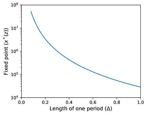
One remaining practical issue is how to numerically compute , which appears in (3.2). By Theorem 2.6(i), is the unique positive solution to the equation , which in principle can be computed using a nonlinear equation solver. However, doing so is not practical because tends to be a very large vector and nonlinear equation solvers tend to terminate before convergence is achieved. For instance, suppose are constant and . Using (2.15), we obtain
Suppose we fix the unit of time somehow (e.g., year), one period has time length , and (with a slight abuse of notation) the discount rate is and the continuously compounded risk-free rate is . Then and , so
| (3.3) |
It is clear that (3.3) diverges to as . In fact, (3.3) tends to be quite large in common settings. For instance, let the unit of time be a year and (4% annual discounting), (3% risk-free rate), and , which are typical values. Figure 1 plots the fixed point (3.3) in the range , which implies that a period is between a month and a year. We can see that tends to be quite large, which makes it impractical to numerically solve for .
A straightforward way to avoid this issue is to directly solve for instead of . Noting that is the fixed point of in (2.7), satisfies
| (3.4) |
To numerically solve the system of equations (3.4) using a nonlinear equation solver, we may use a good initial guess as follows. Conjecture that is approximately equal to for some and that the right Perron vector of is close to 1. Then the equation becomes
Solving for , we obtain
| (3.5) |
Since by assumption, the right-hand side of (3.5) is always in . Therefore we can numerically solve the system of nonlinear equations (3.4) using the initial guess (3.5).
3.2 Updating
Given a candidate consumption function , it is natural to update it to using the Euler equation (2.6). However, this is not generally feasible because is a function and thus is infinite-dimensional. In practice, it is common to set up a finite grid , where are grid points, update by solving for using (2.6) for each , and interpolate (linear, spline, etc.) it if necessary.
Although this updating procedure is theoretically justified, it is not computationally efficient because it requires performing root-finding times for each iteration, which is computationally intensive. A straightforward way to improve the algorithm is to avoid root-finding as in the endogenous grid point method of Carroll (2006).
Instead of fixing a grid for asset, the endogenous grid method fixes a grid for saving , where , update on , and then choose the grid points for asset endogenously based on the optimal consumption and saving. For concreteness, suppose we use linear interpolation and extrapolation. For each , let be the endogenous grid points for asset determined in the -th iteration, where represents the asset grid point when saving is and exogenous state is . We define by for all and . Furthermore, let be the set of continuous piecewise linear functions such that for each , 1. for all , 2. for , 3. is affine in on each subinterval for , and 4. is linearly extrapolated for . Policy iteration for computing the consumption functions via the endogenous grid method can be summarized as follows.
Policy iteration via the endogenous grid method.
- (i)
-
(ii)
(Updating) For each , given , update it as follows:
-
(i)
For each , compute and define
where is computed by linearly interpolating and extrapolating .
-
(ii)
Define the updated asset grid and optimal consumption on by
-
(iii)
Define by linearly interpolating and extrapolating using and setting for .
-
(i)
-
(iii)
(Convergence) Repeat Step (ii) over until the numbers converge.
3.3 Numerical example
To illustrate the computational efficiency of policy iteration, we solve a numerical example in this section.
Model specification
The agent has CRRA utility with constant discount factor and relative risk aversion . There are only two states, so , which we interpret as expansion and recession. Letting be the Markov state at time , labor income is , where is the growth rate of the trend. Suppose the agent invests a constant fraction of wealth into a risky asset whose return is lognormal (with conditional log mean and volatility depending only on the current state ) and the remaining fraction into a risk-free asset. Therefore, the asset return is
| (3.6) |
where and are the conditional log risk premium and volatility, , and is the gross risk-free rate. Although our theory requires a stationary income process, due to homotheticity it is straightforward to allow for a trend. After simple algebra (e.g., Section 2.2 of Carroll, 2021), instead of (2.2), it suffices to use
| (3.7a) | ||||
| (3.7b) | ||||
| (3.7c) | ||||
which are stationary.
We set the parameters as follows. We suppose that one period is a month and set (4% annual discounting) and , which are standard. For the Markov state , we use the 1947-2019 NBER recession indicator444https://fred.stlouisfed.org/series/USREC and estimate the transition probability matrix
from the mean duration of expansions and recessions. For the asset return in (3.6), we set , which is close to the calibrated value in Ma and Toda (2021), and use the spreadsheet of Welch and Goyal (2008)555http://www.hec.unil.ch/agoyal/docs/PredictorData2019.xlsx to construct real log returns and estimate (annual rate 0.63%), , and . The growth rate is computed from the real per capita GDP growth.666https://fred.stlouisfed.org/series/A939RX0Q048SBEA Finally, we set to make the graphs stand out. For computational purposes, we discretize the iid shock using the 7-point Gauss-Hermite quadrature.
Consumption functions and asymptotic MPCs
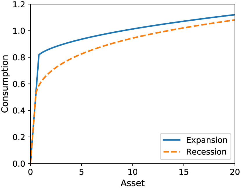
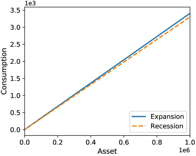
We solve for consumption functions by policy iteration on a 1,000-point exponential grid for saving in the range of .777See Appendix B for the construction of the exponential grid, which is based on Gouin-Bonenfant and Toda (2018). We use the median grid point . We choose the convergence criterion such that policy iteration stops when the maximum relative change from the previous iteration satisfies
At a small scale (Figure 2(a)), the consumption functions show a concave pattern, which is consistent with Carroll and Kimball (1996). At a large scale (Figure 2(b)), the consumption functions look linear, which is consistent with Theorem 2.6 and Proposition 2.8.
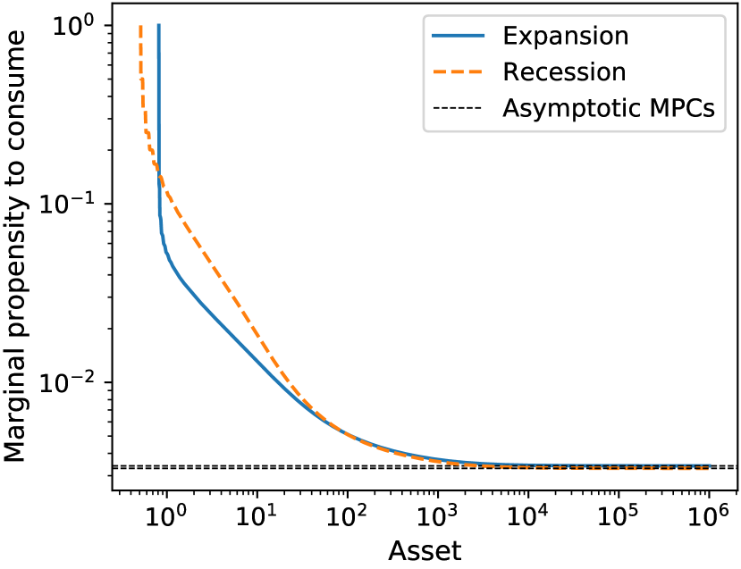
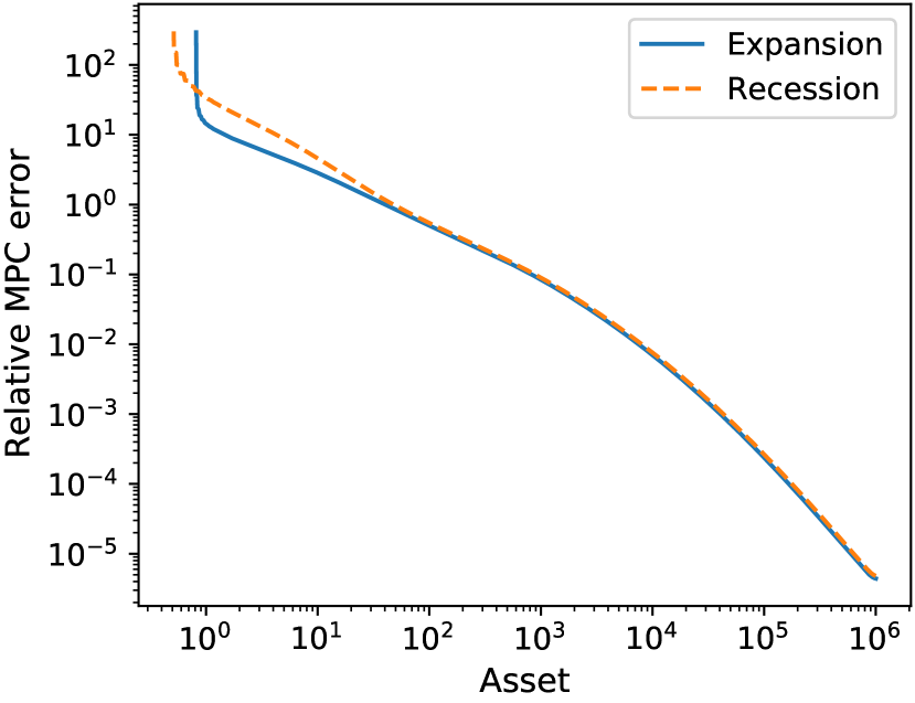
To evaluate how fast the slope of converges to as , we compute the marginal propensities to consume (MPCs) and their relative errors. At the grid point , the MPC and its relative error are defined as888It makes intuitive sense to evaluate MPC on the endogenous asset grid points. In particular, the continuity of the consumption function implies that as (see, for example, Step (ii)(ii)ii of the policy iteration algorithm).
respectively. Figure 3(a) shows the numerical and asymptotic MPCs. Consistent with theory, the MPCs appear to converge to the theoretical values.999Although not visible from Figure 3(a), it is clear from Figure 2(b) that each state has its own limit: we have . Figure 3(b) shows that the relative errors are quite small beyond (around ).
The impact of maximum saving grid
As discussed above, to compute the consumption function numerically, the state space has to be finite. Therefore, it is important to know how to set up the grid points effectively in practice. To answer this question, we study how the choice of the maximum grid point for saving affects the accuracy of the calculated consumption functions.
Our experiment is as follows: First, we treat the consumption function in the previous section as the true consumption function, because it is calculated on a relatively large saving space with and a fine exponential grid of points. We then truncate the grid points for saving to , where is the truncation point. Once this is done, for each , we compute the consumption function on the truncated grid , which we denote as , and calculate its error relative to the true consumption function via
where with a slight abuse of notation, we use to denote the endogenous asset grid points calculated from the true consumption function . The relative error as a function of the truncation point is displayed in Figure 4.
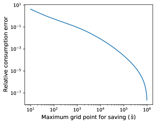
As can be seen from Figure 4, the error of relative to reduces greatly as the maximum grid point for saving gets larger and becomes reasonably small for (below ). Intuitively, smaller saving spaces typically imply that the MPCs at the boundary endogenous asset grid points are further away from their theoretical asymptotes. Therefore, extrapolating consumption outside of the truncated space would result in larger errors. In particular, using small grids such as results in very large errors.101010For instance, Heaton and Lucas (1997) use a 7-point grid on for wealth to solve for consumption functions, which are likely to be inaccurate.
Computational efficiency
To evaluate the computational efficiency of the policy iteration algorithm, we now solve for the consumption functions with various specifications for the number of grid points and initial condition. Same as before, we terminate the policy iteration algorithm at precision . The number of grid points is . To see how the initial guess affects the convergence speed, instead of (3.2), we set
| (3.8) |
where and . For instance, setting amounts to using , while setting amounts to using (3.2). A low value of implies that we choose an initial guess that has an asymptotic slope closer to the true solution.
Table 1 shows the number of iterations and computing time (in seconds) required for convergence for each specification. To calculate these statistics, in each case we repeat the same solution process times and then take the average. We see that that using a theoretically motivated initial guess (3.2) instead of speeds up the algorithm by about to times. The enhanced computational efficiency is largely because the initial guess (3.2) stays closer to the true consumption function compared with , in which case policy iteration converges within fewer steps. Furthermore, because the policy iteration algorithm avoids costly root-finding, the computing time is relatively insensitive to the number of grid points.
| Iterations | Time | Iterations | Time | Iterations | Time | |
|---|---|---|---|---|---|---|
| 1 | 1,716 | 0.66 | 1,714 | 0.64 | 1,712 | 2.86 |
| 0.5 | 1,715 | 0.58 | 1,713 | 0.62 | 1,711 | 2.96 |
| 0.2 | 1,712 | 0.57 | 1,710 | 0.62 | 1,708 | 2.87 |
| 0.1 | 1,707 | 0.85 | 1,705 | 0.62 | 1,703 | 2.91 |
| 0.01 | 1,630 | 0.53 | 1,628 | 0.60 | 1,627 | 2.77 |
| 0.001 | 1,278 | 0.44 | 1,276 | 0.49 | 1,275 | 2.14 |
| 0 | 958 | 0.36 | 1,100 | 0.39 | 1,286 | 2.16 |
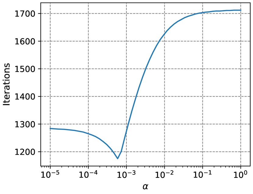
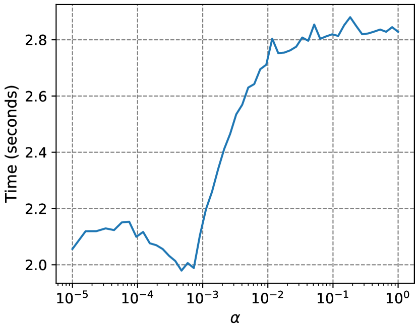
Seen from Table 1, it is fair to predict that policy iteration tends to be more time-consuming as becomes larger. Figure 5 plots the steps and time taken for policy iteration to converge over a fine grid for and inspects this conjecture. In particular, we fix the number of grid points for saving at and use an exponential grid for in the range of with points. Same to Table 1, we repeat the solution process times for each specification and calculate the mean computing time. Figure 5(a) shows that the step for policy iteration to converge is strictly increasing in unless takes very small values (lower than ), while Figure 5(b) reveals a clear increasing trend in computing time as gets larger. Intuitively, since a higher tends to shift the initial guess further away from the true consumption function, policy iteration will take more steps to converge and the problem will be more computationally intensive.
4 Concluding remarks
In this paper, we have systematically studied the asymptotic behavior of the consumption function when the marginal utility is regularly varying. We have shown that the optimal consumption function of the finite horizon optimal savings problem is always asymptotically linear in wealth. For infinite horizon problem, we have derived an asymptotic upper bound for MPC and shown that, whenever the spectral radius condition holds and the limit infimum of MPC as asset tends to infinity is positive, the consumption function is asymptotically linear in wealth and the asymptotic MPC coincides with the upper bound we establish. Furthermore, we have established a list of sufficient conditions for asymptotic linearity based on bounded relative risk aversion or asymptotic constant relative risk aversion.
Our results build a theoretical foundation for linearly extrapolating consumption outside the grid points when solving the optimal savings problem numerically. This in turn allows us to construct good initial guesses for policy iteration and solve the problem efficiently and accurately. Our numerical experiments have demonstrated that working with the initial guess defined in (3.2) speeds up computation obviously and that working with a large saving/asset space created by exponential grid is necessary for improving solution accuracy.
Appendix A Proofs
We need the following result to prove Proposition 2.3.
Theorem A.1 (Representation Theorem).
Let be measurable. Then is slowly varying if and only if it may be written in the form
| (A.1) |
for for some , where are measurable functions such that and as .
Proof.
See Bingham et al. (1987, Theorem 1.3.1). ∎
Proof of Proposition 2.3.
Step 1.
.
If is asymptotically CRRA with coefficient , by definition we can write
where as . Dividing both sides by and integrating on , we obtain
Therefore by Theorem A.1, is regularly varying with index by setting with defined by (A.1) with and .
Step 2.
.
Consider the marginal utility function for in (A.1), where
for some and . Noting that ,111111See Hardy (1909) for an interesting discussion of this integral. we have as , so by Theorem A.1, is slowly varying and . However, log differentiating , we obtain
so always but does not converge as . Therefore .
Step 3.
.
If is regularly varying with index , by Theorem A.1 we can write with as in (A.1). Take any . Since as , we can take such that for . Then
Dividing both sides by and letting , noting that as , we obtain
Since is arbitrary, letting , we obtain
Therefore because , and by definition has an asymptotic exponent .
Step 4.
.
Consider the marginal utility function , where . Then
as , so . Furthermore, by log differentiating , we obtain
so always. To show , it suffices to show that is not slowly varying. Take and . Then
which does not converge as . Therefore is not slowly varying. ∎
Before proving Theorems 2.5 and 2.6, we first proceed heuristically to motivate what the value of should be if it exists. Assuming that the borrowing constraint does not bind, the Euler equation (2.6) implies
where . Multiplying both sides by , setting motivated by (2.10), letting , using Assumption 3 (regular variation), and interchanging expectations and limits, it must be
Dividing both sides by and setting , we obtain
| (A.2) |
Noting that
| (A.3) |
and using the definition of in (2.3), we can rewrite (A.2) as , where is defined in (2.7).
We apply policy function iteration to prove Theorems 2.5 and 2.6. Let be the space of candidate consumption functions as defined in Section 2.1. We further restrict the candidate space to satisfy asymptotic linearity:
| (A.4) |
Clearly is nonempty because belongs to .
The following proposition shows that the operator defined in Section 2.1 maps the candidate space into itself and also shows how the asymptotic MPCs of and are related.
Proposition A.2.
To prove Proposition A.2, we need the following lemma.
Lemma A.3.
Proof.
Suppose . Take any numbers such that . Since as , there exists such that for . Since is strictly decreasing by Assumption 1, it follows that for . Dividing both sides by , letting , and using Assumption 3, we obtain
Letting , we obtain (A.6).
If , take any . By the same argument as above, we obtain
so letting , we obtain (A.6) (and both sides are ). ∎
Proof of Proposition A.2.
Let and .
For , define
| (A.7) |
By Assumption 1, if , then is continuous and strictly decreasing in with and . If , then is continuous and strictly decreasing in with and . In either case, by the intermediate value theorem, for each , there exists a unique such that . By the definition of , we have , where . Therefore .
If almost surely conditional on , then (A.7) becomes
Since solves , it must be . Therefore in particular exists and (A.5) is trivial. Below, assume with positive probability conditional on .
Take any accumulation point of as , which always exists because . Then we can take an increasing sequence such that . Define and
| (A.8) |
By the definitions of and , we have
| (A.9) |
Step 1.
For in (A.8), we have
| (A.10) |
To see this, if and , then since , by the definition of we have
which is (A.10). If or , then since , we have
so again (A.10) holds.
Step 2.
For any accumulation point of as , we have .
Letting in (A.9), applying Lemma A.3, and using the continuity of max and min operators, we obtain
| (A.11) |
where the last equation uses (because ). Applying Fatou’s Lemma, (A.10), and Lemma A.3, it follows from (A.11) that
| (A.12) |
Since by assumption with positive probability conditional on and for all (because ; see (A.4)), it follows that . Therefore solving the inequality (A.12), we obtain
Step 3.
The limit and the expectation can be interchanged in (A.11).
Note that
| (A.13) |
When computing the expectation (A.13), we can divide it into the events and . When , the integrand is zero. When , by Assumption 4, we have . By the definition of and the monotonicity of consumption functions established in Ma et al. (2020), it follows from the definition of in (A.8) that
Since for all , , and is a finite set, for any
there exists such that for all and . Then by Assumptions 1 and 3, for we have
as . Therefore for any , we have
for large enough . Since by Assumption 2 we have whenever , it follows from (A.11), the dominated convergence theorem, and Lemma A.3 that
| (A.14) |
Step 4.
The limit (A.5) holds.
Since the left-hand side of (A.14) is strictly decreasing in and the right-hand side is weakly increasing in , the number that solves (A.14) is unique. Since is any accumulation point of as , it follows that exists. Therefore it only remains to show that the limit equals the right-hand side of (A.5).
Proof of Theorem 2.5.
Proof of Theorem 2.6.
Lemma B.4 of Ma et al. (2020) shows that is order preserving, that is, implies . Define the sequence by and for all . Since , in particular we have , where is as in (A.4). Therefore by Proposition A.2, we have for all , so exists. Since for any , in particular , so by induction for all . Define , which exists because is monotonically decreasing and . Then by Theorem 2.2 of Ma et al. (2020), this is the unique fixed point of and also the unique solution to the optimal savings problem (2.1). Since point-wise, by Proposition A.2 we have
| (A.15) |
where is as in Theorem 2.5.
Case 1: and is irreducible.
Case 2: .
By Proposition 14 of Ma and Toda (2021), we have , where is the unique fixed point of in (2.7). Letting in (A.15), we obtain
which is (2.9). If for all , we can take such that . Therefore we can take such that for . Define . Since is increasing and continuous in and , we have . Furthermore, define
as in Figure 6.
By definition, point-wise. Let us show that . Since is increasing and continuous in , so is . Clearly . Because and for , we have
Since , , and is decreasing, we have
Since is a finite set, we have
so . Since for , we have as , so .
Proof of Theorem 2.7.
Restrict the candidate space to
| (A.16) |
Clearly is nonempty because belongs to . Let us show that . Suppose to the contrary that . Then there exists such that for some and , we have .
Since is strictly decreasing and , it follows from (2.6) that
| (A.17) |
If , then
which is a contradiction. Therefore , and (A.17) becomes
| (A.18) |
As in the proof of Proposition A.2, the event does not affect the expectations in (2.12) and (A.18). Therefore without loss of generality we may assume by Assumption 4. Then by , , , and (2.11), we have
Using the fact that is strictly decreasing and , it follows from (A.18) and that
which contradicts (2.12). Therefore .
Proof of Proposition 2.11.
Let be the unique fixed point of in (2.7), which necessarily satisfies for all . Then
| (A.19) |
Take any and define . Then
| (A.20) |
Again we may assume by Assumption 4. Noting that , where
and are finitely many fixed numbers in , it follows that uniformly as . Since is aCRRA, we have uniformly as . Since and , we can take such that
for , where the last equation follows from (A.19). Combined with (A.20), we obtain for . Therefore (2.12) holds for . Finally, (2.11) holds if is large enough.
If , then we can take such that for all , so (2.11) holds for any . ∎
Appendix B Exponential grid
In many models, the state variable may become negative (e.g., asset holdings), which causes a problem for constructing an exponentially-spaced grid because we cannot take the logarithm of a negative number. Suppose we would like to construct an -point exponential grid on a given interval . A natural idea to deal with such a case is as follows.
Constructing exponential grid.
-
(i)
Choose a shift parameter .
-
(ii)
Construct an -point evenly-spaced grid on .
-
(iii)
Take the exponential.
-
(iv)
Subtract .
The remaining question is how to choose the shift parameter . Suppose we would like to specify the median grid point as . Since the median of the evenly-spaced grid on is , we need to take such that
Note that in this case
so is positive if and only if . Therefore, for any , it is possible to construct an exponentially-spaced grid with end points and median point .
References
- Benhabib et al. (2015) Jess Benhabib, Alberto Bisin, and Shenghao Zhu. The wealth distribution in Bewley economies with capital income risk. Journal of Economic Theory, 159(A):489–515, September 2015. doi:10.1016/j.jet.2015.07.013.
- Bingham et al. (1987) Nicholas H. Bingham, Charles M. Goldie, and Jozef L. Teugels. Regular Variation, volume 27 of Encyclopedia of Mathematics and Its Applications. Cambridge University Press, 1987.
- Brock and Gale (1969) William A. Brock and David Gale. Optimal growth under factor augmenting progress. Journal of Economic Theory, 1(3):229–243, October 1969. doi:10.1016/0022-0531(69)90032-5.
- Cagetti and De Nardi (2006) Marco Cagetti and Mariacristina De Nardi. Entrepreneurship, frictions, and wealth. Journal of Political Economy, 114(5):835–870, October 2006. doi:10.1086/508032.
- Carroll (2006) Christopher D. Carroll. The method of endogenous gridpoints for solving dynamic stochastic optimization problems. Economics Letters, 91(3):312–320, June 2006. doi:10.1016/j.econlet.2005.09.013.
- Carroll (2021) Christopher D. Carroll. Theoretical foundations of buffer stock saving. Quantitative Economics, 2021. Forthcoming.
- Carroll and Kimball (1996) Christopher D. Carroll and Miles S. Kimball. On the concavity of the consumption function. Econometrica, 64(4):981–992, July 1996. doi:10.2307/2171853.
- Chamberlain and Wilson (2000) Gary Chamberlain and Charles A. Wilson. Optimal intertemporal consumption under uncertainty. Review of Economic Dynamics, 3(3):365–395, July 2000. doi:10.1006/redy.2000.0098.
- De Nardi et al. (2010) Mariacristina De Nardi, Eric French, and John B. Jones. Why do the elderly save? the role of medical expenses. Journal of Political Economy, 118(1):39–75, February 2010. doi:10.1086/651674.
- Deaton and Laroque (1992) Angus Deaton and Guy Laroque. On the behaviour of commodity prices. Review of Economic Studies, 59(1):1–23, January 1992. doi:10.2307/2297923.
- Deaton and Laroque (1996) Angus Deaton and Guy Laroque. Competitive storage and commodity price dynamics. Journal of Political Economy, 104(5):896–923, October 1996. doi:10.1086/262046.
- Fagereng et al. (2019) Andreas Fagereng, Martin Blomhoff Holm, Benjamin Moll, and Gisle Natvik. Saving behavior across the wealth distribution: The importance of capital gains. 2019.
- Gouin-Bonenfant and Toda (2018) Émilien Gouin-Bonenfant and Alexis Akira Toda. Pareto extrapolation: An analytical framework for studying tail inequality. 2018. URL https://ssrn.com/abstract=3260899.
- Guner et al. (2012) Nezih Guner, Remzi Kaygusuz, and Gustavo Ventura. Taxation and household labour supply. Review of Economic Studies, 79(3):1113–1149, July 2012. doi:10.1093/restud/rdr049.
- Guvenen (2011) Fatih Guvenen. Macroeconomics with heterogeneity: A practical guide. NBER Working Paper 17622, 2011. URL http://www.nber.org/papers/w17622.
- Guvenen and Smith (2014) Fatih Guvenen and Anthony A. Smith, Jr. Inferring labor income risk and partial insurance from economic choices. Econometrica, 82(6):2085–2129, November 2014. doi:10.3982/ECTA9446.
- Hardy (1909) Godfrey H. Hardy. The integral . Mathematical Gazette, 5(80):98–103, June 1909. doi:10.2307/3602798.
- Heathcote et al. (2014) Jonathan Heathcote, Kjetil Storesletten, and Giovanni L. Violante. Consumption and labor supply with partial insurance: An analytical framework. American Economic Review, 104(7):2075–2126, July 2014. doi:10.1257/aer.104.7.2075.
- Heaton and Lucas (1997) John Heaton and Deborah Lucas. Market frictions, savings behavior, and portfolio choice. Macroeconomic Dynamics, 1(1):76–101, January 1997. doi:10.1017/S1365100597002034.
- Holm (2018) Martin Blomhoff Holm. Consumption with liquidity constraints: An analytical characterization. Economics Letters, 167:40–42, June 2018. doi:10.1016/j.econlet.2018.03.004.
- Huggett (1993) Mark Huggett. The risk-free rate in heterogeneous-agent incomplete-insurance economies. Journal of Economic Dynamics and Control, 17(5-6):953–969, September-November 1993. doi:10.1016/0165-1889(93)90024-M.
- Krusell and Smith (1998) Per Krusell and Anthony A. Smith, Jr. Income and wealth heterogeneity in the macroeconomy. Journal of Political Economy, 106(5):867–896, October 1998. doi:10.1086/250034.
- Lehrer and Light (2018) Ehud Lehrer and Bar Light. The effect of interest rates on consumption in an income fluctuation problem. Journal of Economic Dynamics and Control, 94:63–71, September 2018. doi:10.1016/j.jedc.2018.07.004.
- Li and Stachurski (2014) Huiyu Li and John Stachurski. Solving the income fluctuation problem with unbounded rewards. Journal of Economic Dynamics and Control, 45:353–365, August 2014. doi:10.1016/j.jedc.2014.06.003.
- Light (2018) Bar Light. Precautionary saving in a Markovian earnings environment. Review of Economic Dynamics, 29:138–147, July 2018. doi:10.1016/j.red.2017.12.004.
- Light (2020) Bar Light. Uniqueness of equilibrium in a Bewley-Aiyagari economy. Economic Theory, 69:435–450, 2020. doi:10.1007/s00199-018-1167-z.
- Ma and Toda (2021) Qingyin Ma and Alexis Akira Toda. A theory of the saving rate of the rich. Journal of Economic Theory, 192:105193, March 2021. doi:10.1016/j.jet.2021.105193.
- Ma et al. (2020) Qingyin Ma, John Stachurski, and Alexis Akira Toda. The income fluctuation problem and the evolution of wealth. Journal of Economic Theory, 187:105003, May 2020. doi:10.1016/j.jet.2020.105003.
- Rabault (2002) Guillaume Rabault. When do borrowing constraints bind? Some new results on the income fluctuation problem. Journal of Economic Dynamics and Control, 26(2):217–245, February 2002. doi:10.1016/S0165-1889(00)00042-7.
- Samuelson (1969) Paul A. Samuelson. Lifetime portfolio selection by dynamic stochastic programming. Review of Economics and Statistics, 51(3):239–246, August 1969. doi:10.2307/1926559.
- Schechtman and Escudero (1977) Jack Schechtman and Vera L. S. Escudero. Some results on “an income fluctuation problem”. Journal of Economic Theory, 16(2):151–166, December 1977. doi:10.1016/0022-0531(77)90003-5.
- Stachurski and Toda (2019) John Stachurski and Alexis Akira Toda. An impossibility theorem for wealth in heterogeneous-agent models with limited heterogeneity. Journal of Economic Theory, 182:1–24, July 2019. doi:10.1016/j.jet.2019.04.001.
- Stachurski and Toda (2020) John Stachurski and Alexis Akira Toda. Corrigendum to “An impossibility theorem for wealth in heterogeneous-agent models with limited heterogeneity” [Journal of Economic Theory 182 (2019) 1–24]. Journal of Economic Theory, 188:105066, July 2020. doi:10.1016/j.jet.2020.105066.
- Toda (2019) Alexis Akira Toda. Wealth distribution with random discount factors. Journal of Monetary Economics, 104:101–113, June 2019. doi:10.1016/j.jmoneco.2018.09.006.
- Toda (2020) Alexis Akira Toda. Necessity of hyperbolic absolute risk aversion for the concavity of consumption functions. Journal of Mathematical Economics, 2020. doi:10.1016/j.jmateco.2020.102460.
- Welch and Goyal (2008) Ivo Welch and Amit Goyal. A comprehensive look at the empirical performance of equity premium prediction. Review of Financial Studies, 21(4):1455–1508, July 2008. doi:10.1093/rfs/hhm014.
- Zeldes (1989) Stephen P. Zeldes. Optimal consumption with stochastic income: Deviations from certainty equivalence. Quarterly Journal of Economics, 104(2):275–298, May 1989. doi:10.2307/2937848.