Asymptotic expansion for the Hartman-Watson distribution

Dan Pirjol School of Business
Stevens Institute of Technology
Hoboken, NJ 07030 [email protected]

(Date: 20 February 2021)

Abstract.

The Hartman-Watson distribution with density $f_{r}(t)=\frac{1}{I_{0}(r)}\theta(r,t)$ with $r>0$ is a probability distribution defined on $t\geq 0$ which appears in several problems of applied probability. The density of this distribution is expressed in terms of an integral $\theta(r,t)$ which is difficult to evaluate numerically for small $t\to 0$ . Using saddle point methods, we obtain the first two terms of the $t\to 0$ expansion of $\theta(\rho/t,t)$ at fixed $\rho>0$ . An error bound is obtained by numerical estimates of the integrand, which is furthermore uniform in $\rho$ . As an application we obtain the leading asymptotics of the density of the time average of the geometric Brownian motion as $t\to 0$ . This has the form $\mathbb{P}(\frac{1}{t}\int_{0}^{t}e^{2(B_{s}+\mu s)}ds\in da)\sim(2\pi t)^{-\frac{1}{2}}g(a,\mu)e^{-\frac{1}{t}J(a)}\frac{da}{a}$ , with an exponent $J(a)$ which reproduces the known result obtained previously using Large Deviations theory.

Key words and phrases:

Asymptotic expansions, saddle point method, linear functional of the geometric Brownian motion

1. Introduction

The Hartman-Watson distribution was introduced in the context of directional statistics [15] and was studied further in relation to the first hitting time of certain diffusion processes [17]. This distribution has received considerable attention due to its relation to the law of the time integral of the geometric Brownian motion, see Eq. (3) below [25].

The Hartman-Watson distribution is given in terms of the function $\theta(r,t)$ defined as

(1)

\theta(r,t)=\frac{r}{\sqrt{2\pi^{3}t}}e^{\frac{\pi^{2}}{2t}}\int_{0}^{\infty}e^{-\frac{\xi^{2}}{2t}}e^{-r\cosh\xi}\sinh\xi\sin\frac{\pi\xi}{t}d\xi\,.

The normalized function $f_{r}(t)=\frac{\theta(r,t)}{I_{0}(r)}$ defines the density of a random variable taking values on the positive real axis $t\geq 0$ , called the Hartman-Watson law [15].

The function $\theta(r,t)$ is related to the distribution of the time-integral of a geometric Brownian motion. Define

(2)

A_{t}^{(\mu)}=\int_{0}^{t}e^{2(B_{s}+\mu s)}ds

with $B_{t}$ a standard Brownian motion and $\mu\in\mathbb{R}$ . The time-integral of the geometric Brownian motion is relevant for the pricing of Asian options in the Black-Scholes model [10], and appears also in actuarial science [5] and in the study of diffusion processes in random media [7]. Other applications to mathematical finance are related to the distributional properties of stochastic volatility models with log-normally distributed volatility, such as the $\beta=1$ log-normal SABR model [1, 6] and the Hull-White model [13, 14].

An explicit result for the joint distribution of $(A_{t}^{(\mu)},B_{t})$ was given by Yor [25]

(3)

\displaystyle\mathbb{P}(A_{t}^{(\mu)}\in du,B_{t}+\mu t\in dx)=e^{\mu x-\frac{1}{2}\mu^{2}t}\exp\left(-\frac{1+e^{2x}}{2u}\right)\theta(e^{x}/u,t)\frac{dudx}{u}\,,

where the function $\theta(r,t)$ is given by (1).

The Yor formula (3) yields also the density of $A_{t}^{(\mu)}$ by integration over $B_{t}$ . The usefulness of this approach is limited by issues with the numerical evaluation of the integral in (1) for small $t$ , due to the rapidly oscillating factor $\sin(\pi\xi/t)$ [3, 5]. Alternative numerical approaches which avoid this issue were presented in [4, 16].

For this reason considerable effort has been devoted to applying analytical methods to simplify Yor’s formula. For particular cases $\mu=0,1$ simpler expressions as single integrals have been obtained for the density of $A_{t}^{(\mu)}$ by Comtet et al [7] and Dufresne [9]. See the review article by Matsumoto and Yor [19] for an overview of the literature.

In the absence of simple exact analytical results, it is important to have analytical expansions of $\theta(r,t)$ in the small- $t$ region. Such an expansion has been derived by Gerhold in [12], by a saddle point analysis of the Laplace inversion integral of the density $f_{r}(t)$ .

In this paper we derive the $t\to 0$ asymptotics of the function $\theta(r,t)$ at fixed $rt=\rho$ using the saddle point method. This regime is important for the study of the small- $t$ asymptotics of the density of $\frac{1}{t}A_{t}^{(\mu)}$ following from the Yor formula (3). The resulting expansion turns out to give also a good numerical approximation of $\theta(r,t)$ for all $t\geq 0$ . The expansion has the form

(4)

\theta(\rho/t,t)=\frac{1}{2\pi t}e^{-\frac{1}{t}\left(F(\rho)-\frac{\pi^{2}}{2}\right)}\left(G(\rho)+G_{1}(\rho)t+O(t^{2})\right)\,.

The leading order term proportional to $G(\rho)$ is given in Proposition 1, and the subleading correction $G_{1}(\rho)$ is given in the Appendix.

The paper is structured as follows. In Section 2 we present the leading order asymptotic expansion of the integral $\theta(r,t)$ at fixed $\rho=rt$ . The main result is Proposition 1. An explicit error bound for the leading term in the asymptotic expansion of $\theta(\rho/t,t)$ is given, guided by numerical tests, which is furthermore uniformly bounded in $\rho$ . In Section 3 we compare this asymptotic result with existing results in the literature on the small $t$ expansion of the Hartman-Watson distribution [3, 12]. In Section 4 we apply the expansion to obtain the leading $t\to 0$ asymptotics of the density of the time averaged geometric Brownian motion $\mathbb{P}(\frac{1}{t}\int_{0}^{t}e^{2(B_{s}+\mu s)}ds\in da)=f(a,t)\frac{da}{a}$ . The leading asymptotics of this density has the form $f(a,t)\sim(2\pi t)^{-\frac{1}{2}}g(a,\mu)e^{-\frac{1}{t}J(a)}$ . The exponential factor $J(a)$ reproduces a known result obtained previously using Large Deviations theory [2, 21]. An Appendix gives an explicit result for the subleading correction.

2. Asymptotic expansion of $\theta(\rho/t,t)$ as $t\to 0$

We study here the asymptotics of $\theta(r,t)$ as $t\to 0$ at fixed $rt=\rho$ . This regime is different from that considered in [12], which studied the asymptotics of $\theta(r,t)$ as $t\to 0$ at fixed $r$ .

Proposition 1.

The $t\to 0$ asymptotics of the Hartman-Watson integral $\theta(\rho/t,t)$ is

(5)

\theta(\rho/t,t)=\frac{1}{2\pi t}e^{-\frac{1}{t}\left(F(\rho)-\frac{\pi^{2}}{2}\right)}\left(G(\rho)+G_{1}(\rho)t+O(t^{2})\right)\,,\quad t\to 0\,.

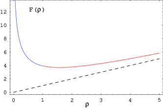
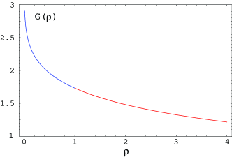
The function $F(\rho)$ is given by

(9)

\displaystyle F(\rho)=\left\{\begin{array}[]{cc}\frac{1}{2}x_{1}^{2}-\rho\cosh x_{1}+\frac{\pi^{2}}{2}&\,,0<\rho<1\\ -\frac{1}{2}y_{1}^{2}+\rho\cos y_{1}+\pi y_{1}&\,,\rho>1\\ \frac{\pi^{2}}{2}-1&\,,\rho=1\\ \end{array}\right.

and the function $G(\rho)$ is given by

(13)

\displaystyle G(\rho)=\left\{\begin{array}[]{cc}\frac{\rho\sinh x_{1}}{\sqrt{\rho\cosh x_{1}-1}}&\,,0<\rho<1\\ \frac{\rho siny_{1}}{\sqrt{1+\rho\cos y_{1}}}&\,,\rho>1\\ \sqrt{3}&\,,\rho=1\\ \end{array}\right.

Here $x_{1}$ is the solution of the equation

(14)

\rho\frac{\sinh x_{1}}{x_{1}}=1

and $y_{1}$ is the solution of the equation

(15)

y_{1}+\rho\sin y_{1}=\pi\,.

The subleading correction is $G_{1}(\rho)=\frac{1}{2}G(\rho)\tilde{g}_{2}(\rho)$ where $\tilde{g}_{2}(\rho)$ is given in explicit form in the Appendix.

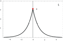
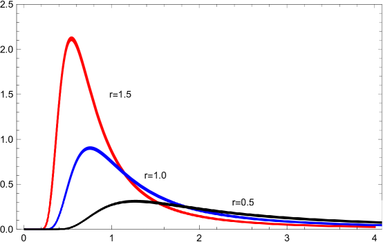
Plots of the functions $F(\rho)$ and $G(\rho)$ are shown in Figure 1. The properties of these functions are studied in more detail in Section 2.2.

Refer to caption — Figure 1. Left: Plot of $F(\rho)$ given in Eq. (9). The two branches in Eq. (9) are shown as the blue and red curves, respectively. The function $F(\rho)$ has a minimum at $\rho=\frac{\pi}{2}$ , with $F(\frac{\pi}{2})=\frac{3\pi^{2}}{8}$ . The dashed line shows the asymptotic line $F(\rho)\sim\rho$ for $\rho\to\infty$ . Right: Plot of $G(\rho)$ defined in Eq. (13).

Proof of Proposition 1.

The function $\theta(\rho/t,t)$ can be written as

(16)		$\displaystyle\theta(\rho/t,t)=\frac{\rho/t}{\sqrt{2\pi^{3}t}}e^{\frac{\pi^{2}}{2t}}\int_{0}^{\infty}e^{-\frac{1}{t}[\frac{1}{2}\xi^{2}+\rho\cosh\xi]}\sinh\xi\sin\frac{\pi\xi}{t}d\xi$
	$\displaystyle=\frac{\rho/t}{\sqrt{2\pi^{3}t}}e^{\frac{\pi^{2}}{2t}}\frac{1}{2}\int_{-\infty}^{\infty}e^{-\frac{1}{t}[\frac{1}{2}\xi^{2}+\rho\cosh\xi]}\sinh\xi\sin\frac{\pi\xi}{t}d\xi$
	$\displaystyle=\frac{\rho}{\sqrt{2\pi^{3}t^{3}}}e^{\frac{\pi^{2}}{2t}}\frac{1}{4i}(I_{+}(\rho,t)-I_{-}(\rho,t))\,,$

with

(17)

I_{\pm}(\rho,t):=\int_{-\infty}^{\infty}e^{-\frac{1}{t}[\frac{1}{2}\xi^{2}+\rho\cosh\xi\mp i\pi\xi]}\sinh\xi d\xi\,.

These integrals have the form $\int_{\alpha}^{\beta}e^{-\frac{1}{t}h(\xi)}g(\xi)d\xi$ with $h_{\pm}(\xi)=\frac{1}{2}\xi^{2}+\rho\cosh\xi\mp i\pi\xi$ .

The asymptotics of $I_{\pm}(t)$ as $t\to 0$ can be obtained using the saddle-point method, see for example Sec. 4.6 in Erdélyi [11] and Sec. 4.7 of Olver [20].

We present in detail the asymptotic expansion for $t\to 0$ of the integral

(18)

I_{+}(\rho,t)=\int_{-\infty}^{\infty}e^{-\frac{1}{t}h(\xi)}\sinh\xi d\xi

where we denote for simplicity $h(\xi)=h_{+}(\xi)=\frac{1}{2}\xi^{2}+\rho\cosh\xi-i\pi\xi$ . The integral $I_{-}(\rho,t)$ is treated analogously.

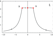
i) $0<\rho<1$ . The saddle points are given by the solution of the equation $h^{\prime}(\xi)=0$ . There are three saddle points at $\xi=\{i\pi,i\pi\pm x_{1}\}$ with $x_{1}$ the solution of the equation $x_{1}-\rho\sinh x_{1}=0$ . The second derivative of $h$ at these points is $h^{\prime\prime}(i\pi)=1-\rho>0$ , and $h^{\prime\prime}(i\pi\pm x_{1})=1-\rho\cosh x_{1}<0$ .

The contour of integration is deformed from the real axis to the contour shown in the left panel of Fig. 2, consisting of three arcs of curves of steepest descent passing through the three saddle points. Along these arcs we have $Im[h(\xi)]=x(y-\pi)+\rho\sinh x\sin y=0$ . Denoting $\xi=x+iy$ , the path is given by

(21)

\displaystyle y=\left\{\begin{array}[]{cc}\pi&\,,|x|\leq x_{1}\\ y_{0}(x)&\,,|x|>x_{1}\\ \end{array}\right.

where $y_{0}(x)$ is the positive solution of the equation $\rho\sinh x\sin y=(\pi-y)x$ .

The integral is a sum of three integrals along each piece of the path. The real part of the integrand is odd and the imaginary part is even under $x\to-x$ . This follows from noting that we have $\mbox{Re}h(-x+iy)=\mbox{Re}h(x+iy)$ and $\sinh(x+iy)=\sinh x\cos y+i\sin y\cosh x$ . This implies that i) the integral from B to A vanishes because the integrand is odd, and ii) the real parts of the integrals along $(-\infty,B]$ and $[A,\infty)$ are equal and of opposite sign, and their imaginary parts are equal. This gives

(22)

\theta(\rho/t,t)=\frac{\rho}{\sqrt{2\pi^{3}t^{3}}}e^{\frac{\pi^{2}}{2t}}\frac{1}{2i}\left(I_{(-\infty,B]}+I_{[A,\infty)}\right)=\frac{\rho}{\sqrt{2\pi^{3}t^{3}}}e^{\frac{\pi^{2}}{2t}}\mbox{Im}I_{[A,\infty)}\,.

Thus it is sufficient to evaluate only $\mbox{Im}I_{[A,\infty)}$ . This integral is written as

(23)

I_{[A,\infty)}(\rho,t)=\int_{A}^{\infty}e^{-\frac{1}{t}h(\xi)}\sinh\xi d\xi=e^{-\frac{1}{t}h(A)}\int_{0}^{\infty}e^{-\frac{1}{t}\tau}\frac{\sinh\xi}{h^{\prime}(\xi)}d\tau\,,

where we defined $\tau=h(\xi)-h(A)$ . This is expanded around $\xi=A$ as

(24)

\tau=h(\xi)-h(A)=a_{2}(\xi-A)^{2}+a_{3}(\xi-A)^{3}+a_{4}(\xi-A)^{4}+O((\xi-A)^{5})

with $a_{2}=\frac{1}{2}h^{\prime\prime}(A),a_{3}=\frac{1}{6}h^{\prime\prime\prime}(A),\cdots$ . Noting $h^{\prime\prime}(A)=1-\rho\cosh x_{1}<0$ , this series is inverted as

(25)

\xi-A=-i\sqrt{\frac{2\tau}{|h^{\prime\prime}(A)|}}+O(\tau)

The second factor in the integrand of (23) is also expanded in $\xi-A$ as

(26)

\frac{\sinh\xi}{h^{\prime}(\xi)}=\frac{\sinh A+\cosh A(\xi-A)+O((\xi-A)^{2})}{h^{\prime\prime}(A)(\xi-A)+O((\xi-A)^{2})}=\frac{\sinh A}{h^{\prime\prime}(A)}\frac{1}{\xi-A}\left(1+O(\xi-A)\right)

Substituting here the expansion (25) gives

(27)

\frac{\sinh\xi}{h^{\prime}(\xi)}=i\frac{\sinh x_{1}}{|h^{\prime\prime}(A)|}\sqrt{\frac{|h^{\prime\prime}(A)|}{2}}\frac{1}{\sqrt{\tau}}+O(\tau^{0})

More generally

(28)

g(\tau)=\frac{\sinh\xi}{h^{\prime}(\xi)}=\frac{g_{0}}{\sqrt{\tau}}+g_{1}+g_{2}\sqrt{\tau}+O(\tau)\,.

The inequality $h^{\prime\prime}(A)<0$ implies that $g_{0},g_{2},\cdots$ are imaginary, while $g_{1},g_{3},\cdots$ are real.

By Watson’s lemma [20], the resulting expansion can be integrated term by term. The leading asymptotic contribution to $I_{[A,\infty)}(\rho,t)$ is

(29)		$\displaystyle\mbox{Im}I_{[A,\infty)}(\rho,t)=e^{-\frac{1}{t}h(A)}\mbox{Im}\int_{0}^{\infty}e^{-\frac{1}{t}\tau}\frac{\sinh\xi}{h^{\prime}(\xi)}d\tau$
	$\displaystyle\qquad=\frac{\sinh x_{1}}{\sqrt{2\|h^{\prime\prime}(A)\|}}e^{-\frac{1}{t}h(A)}\left(\sqrt{\pi t}+O(t^{3/2})\right)\,.$

The leading order term integral was evaluated as $\int_{0}^{\infty}e^{-\frac{1}{t}\tau}\frac{d\tau}{\sqrt{\tau}}=\sqrt{\pi t}$ . Substituting into (22) reproduces the quoted result by identifying $h(A)=F(\rho)$ . Since $g_{1},g_{3},\cdots$ are real, the $O(\tau^{0})$ term in (28) does not contribute to $ImI_{[A,\infty)}$ , and the leading correction comes from the $O(\tau^{1/2})$ term. This is given in explicit form in the Appendix.

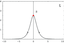
ii) $\rho>1$ . There are several saddle points along the imaginary axis. We are interested in the saddle point at $\xi=iy_{1}$ with $0<y_{1}\leq\pi$ the solution of (15). At this point the second derivative of $h$ is $h^{\prime\prime}(iy_{1})=1+\rho\cos y_{1}>0$ .

Deform the $\xi:(-\infty,+\infty)$ integration contour into the curve in the middle panel of Fig. 2. This is a steepest descent curve $\mbox{Im}(h(\xi))=0$ , given by $y_{0}(x)$ , the positive solution of the equation $\rho\sinh x\sin y=(\pi-y)x$ . The contour passes through the saddle point $S$ at $\xi=iy_{1}$ .

The integral $I_{+}(\rho,t)=\int_{-\infty}^{S}+\int_{S}^{+\infty}$ is the sum of the two integrals on the two halves of the contour. As in the previous case, the sum is imaginary since $h(\xi)$ is real along the contour, and $Re[h(\xi)]$ is even in $x$ . Noting that $\sinh(x+iy)=\sinh x\cos y+i\sin y\cosh x$ , the first term is odd in $x$ and cancels out, and only the second (imaginary) term gives a contribution. We have a result similar to (22)

(30)

\theta(\rho/t,t)=\frac{\rho}{\sqrt{2\pi^{3}t^{3}}}e^{\frac{\pi^{2}}{2t}}\frac{1}{2i}\left(I_{(-\infty,S]}+I_{[S,\infty)}\right)=\frac{\rho}{\sqrt{2\pi^{3}t^{3}}}e^{\frac{\pi^{2}}{2t}}\mbox{Im}I_{[S,\infty)}\,.

As before, it is sufficient to evaluate only the $[S,\infty)$ integral, which is

(31)

I_{[S,\infty)}(\rho,t)=\int_{S}^{\infty}e^{-\frac{1}{t}h(\xi)}\sinh\xi d\xi=e^{-\frac{1}{t}h(S)}\int_{0}^{\infty}e^{-\frac{1}{t}\tau}\frac{\sinh\xi}{h^{\prime}(\xi)}d\tau

where we introduced $\tau=h(\xi)-h(S)\geq 0$ . This difference is expanded around $\xi=S$ as

(32)

\tau=h(\xi)-h(S)=\frac{1}{2}h^{\prime\prime}(S)(\xi-S)^{2}+O((\xi-S)^{3})

which is inverted as (recall $h^{\prime\prime}(S)>0$ )

(33)

\xi-S=\sqrt{\frac{2\tau}{h^{\prime\prime}(S)}}+O(\tau)

The integrand is also expanded in $\xi-S$ as

(34)

\frac{\sinh\xi}{h^{\prime}(\xi)}=\frac{\sinh S+\cosh S(\xi-S)+O((\xi-S)^{2})}{h^{\prime\prime}(S)(\xi-S)+O((\xi-S)^{2})}=\frac{\sinh S}{h^{\prime\prime}(S)}\frac{1}{\xi-S}\left(1+O((\xi-S))\right)\,.

Substituting here (33) this can be expanded in powers of $\sqrt{\tau}$ as

(35)

\frac{\sinh\xi}{h^{\prime}(\xi)}=\frac{g_{0}}{\sqrt{\tau}}+g_{1}+g_{2}\sqrt{\tau}+O(\tau)\,.

As in the previous case, $g_{0},g_{2},\cdots$ are imaginary, while $g_{1},g_{3},\cdots$ are real, such that only the even order terms contribute.

By Watson’s lemma [20] we can exchange expansion and integration, and we get the leading asymptotic term

(36)

Im\int_{0}^{\infty}e^{-\frac{1}{t}\tau}\frac{\sinh\xi}{h^{\prime}(\xi)}d\tau=\frac{\sin y_{1}}{\sqrt{2h^{\prime\prime}(S)}}\left(\sqrt{\pi t}+O(t^{3/2})\right)\,.

The $O(t^{3/2})$ subleading term is given in explicit form in the Appendix.

iii) $\rho=1$ . Some details of proof are different for $\rho=1$ since the saddle point $S$ at $\xi=i\pi$ is of fourth order, so the Taylor expansion of $\tau$ starts with the fourth order term in $\xi-S$

(37)

\tau=h(\xi)-h(S)=\frac{1}{4!}h^{\prime\prime\prime\prime}(S)(\xi-S)^{4}+\cdots\,,\quad h^{\prime\prime\prime\prime}(S)=-1

This expansion in $z:=\xi-S$ can be put in closed form as

(38)

\tau=-\frac{1}{4!}z^{4}-\frac{1}{6!}z^{6}+O(z^{8})=-\cosh z+1+\frac{1}{2}z^{2}\,.

The inversion of this expansion gives

(39)

\displaystyle z=\xi-S

\displaystyle=

\displaystyle(-24\tau)^{1/4}-\frac{1}{120}(-24\tau)^{3/4}+\frac{11}{67200}(-24\tau)^{5/4}+O(\tau^{7/4})\,.

Deform the $\xi:(-\infty,+\infty)$ integration contour as in the right plot of Fig. 2 along the steepest descent curve $\mbox{Im}(h(\xi))=0$ . Denote this curve $y_{0}(x)$ , where $y_{0}(x)$ is the solution satisfying $0<y<\pi$ of $\sinh x\sin y=(\pi-y)x$ . As in the previous cases, it is sufficient to evaluate only the $[S,\infty)$ integral, which has the same form as (31).

The expansion of the integrand starts with an inverse quadratic term

(40)

\frac{\sinh\xi}{h^{\prime}(\xi)}=\frac{\cosh S(\xi-S)+\cdots}{\frac{1}{3!}h^{\prime\prime\prime\prime}(S)(\xi-S)^{3}+\cdots}=\frac{6}{(\xi-S)^{2}}+O((\xi-S)^{3})

Substituting the derivatives $h^{(k)}(S)$ gives an explicit expression for the expansion in $z:=\xi-S$

(41)

\frac{\sinh\xi}{h^{\prime}(\xi)}=\frac{-z-\frac{1}{3!}z^{3}-\frac{1}{5!}z^{5}-O(z^{7})}{-\frac{1}{3!}z^{3}-\frac{1}{5!}z^{5}-O(z^{7})}=\frac{\sinh z}{\sinh z-z}\,.

Substituting the expansion (39) into (40) gives an expansion of the form

(42)

\frac{\sinh\xi}{h^{\prime}(\xi)}=\sqrt{\frac{3}{2}}\frac{1}{\sqrt{-\tau}}+\frac{4}{5}+\frac{1}{35}\sqrt{\frac{3}{2}}\sqrt{-\tau}+O(\tau)

Along the integration path the square root is defined with a negative imaginary part $\sqrt{-\tau}=-i\sqrt{\tau}$ , which gives

(43)

\mbox{Im}\frac{\sinh\xi}{h^{\prime}(\xi)}=\sqrt{\frac{3}{2}}\frac{1}{\sqrt{\tau}}-\frac{1}{35}\sqrt{\frac{3}{2}}\sqrt{\tau}+O(\tau^{3/2})\,.

Thus the expansion is in powers of $\tau$ , rather than fractional powers of $\tau$ .

Application of Watson’s lemma gives the expansion of the integral

(44)

\mbox{Im }\int_{0}^{\infty}e^{-\frac{1}{t}\tau}\frac{\sinh\xi}{h^{\prime}(\xi)}d\tau=e^{-\frac{1}{t}h(S)}\sqrt{\frac{3}{2}\pi t}\left(1-\frac{1}{70}t+O(t^{2})\right)

with $h(S)=\frac{1}{2}\pi^{2}-1$ . As in the previous cases, the expansion is in integer powers of $t$ . The leading term coincides with the $\rho\to 1$ limit of the above two cases. The $O(t)$ subleading term reproduces the first term in Eq. (121) in the Appendix.

∎

The higher order terms $O(t^{j})$ with $j>2$ for case (iii) can be easily computed.

Remark 2.

The expansion for $\rho=1$ takes a particularly simple form. This is an alternating series, and the first three terms are

(45)

\theta(1/t,t)=\frac{\sqrt{3}}{2\pi t}e^{\frac{1}{t}}\left(1-\frac{1}{70}t+\frac{749,033}{1,034,880,000}t^{2}+O(t^{3})\right)

2.1. Error estimates

We examine here the error of the approximation for $\theta(r,t)$ obtained by keeping only the leading asymptotic term in Proposition 1, and give an explicit error bound (53), backed by the results of a numerical study. The bound is uniform in $\rho$ .

Define the remainder of the asymptotic expansion of Proposition 1 as

(46)

\theta(\rho/t,t)=\frac{1}{2\pi t}G(\rho)e^{\frac{1}{t}[F(\rho)-\frac{\pi^{2}}{2}]}\left(1+\vartheta(t,\rho)\right)\,.

First, we note that for all cases (i) $0<\rho<1$ (ii) $\rho>1$ and (iii) $\rho=1$ , the integrand in the application of Watson’s lemma has a similar expansion

(47)

\mbox{Im}g(\xi)=\frac{\mbox{Im}g_{0}(\rho)}{\sqrt{\tau}}+\mbox{Im}g_{2}(\rho)\sqrt{\tau}+O(\tau^{3/2})

see (28), (35) and (43), respectively. The coefficient of the leading order term is

(48)

\mbox{Im}g_{0}(\rho)=\left\{\begin{array}[]{cc}\frac{\sinh x_{1}}{\sqrt{2(\rho\cosh x_{1}-1)}}&\,,0<\rho<1\\ \sqrt{\frac{3}{2}}&\,,\rho=1\\ \frac{\sin y_{1}}{\sqrt{2(1+\rho\cos y_{1})}}&\,,\rho>1\\ \end{array}\right.

We can obtain a bound on the remainder function $\vartheta(t,\rho)$ by examining the approximation error of the integrand $\mbox{Im }g(\xi)$ by the first term in its series expansion (47). Denoting $\xi=x+iy$ we have

(49)

\mbox{Im }g(\xi)=\frac{x\cosh x\sin y+(\pi-y)\cos y\sinh x}{(\rho\cosh x\sin y-\pi+y)^{2}+(x+\rho\cos y\sinh x)^{2}}\,.

Define

(50)

\mbox{Im}\,g(\xi(\tau)):=\frac{\mbox{Im}g_{0}(\rho)}{\sqrt{\tau}}(1+\delta(\tau,\rho))

Numerical testing shows the following properties of the remainder function $\delta(\tau,\rho)$ :

i) $\delta(\tau,\rho)\leq 0$ is negative

ii) $\delta(\tau,\rho)\to-1$ as $\tau\to\infty$ . This follows by expanding $Img(\xi(\tau))$ as $x\to\infty$ along the steepest descent curves $y(x)$ . For $\rho=1$ this curve has the asymptotics $y(x)\simeq 2\pi xe^{-x}$ .

Expressed in terms of $\tau$ we get

(51)

Img(\xi(\tau))=\frac{\pi}{\tau}+O(\tau^{-2})\,,\quad\tau\to\infty\,.

iii) $|\delta(\tau,\rho)|\leq 1$ .

iv) it is bounded in absolute value as

(52)

|\delta(\tau,\rho)|\leq|\tilde{g}_{2}(\rho)|\tau\leq\frac{1}{35}\tau\,,\quad\tau\geq 0

for all $\rho>0$ , where $\tilde{g}_{2}(\rho):=\frac{Img_{2}(\rho)}{Img_{0}(\rho)}$ . An explicit result for $\tilde{g}_{2}(\rho)$ is given in Eq. (120) in the Appendix, and its plot is shown in Fig. 5. Numerical study shows that $|\tilde{g}_{2}(\rho)|$ reaches a maximum value at $\rho=1$ , equal to $\frac{1}{35}$ . This gives a uniform bound, valid for all $\rho>0$ .

We can transfer these results to a bound on the error of the application of Watson’s lemma.

Remark 3.

The error term $\vartheta(t,\rho)$ in (46) is bounded from above as

(53)

|\vartheta(t,\rho)|\leq\frac{1}{2}\cdot\frac{|Img_{2}(\rho)|}{|Img_{0}(\rho)|}t\leq\frac{1}{70}t\,,

with $g_{0}(\rho),g_{2}(\rho)$ the coefficients in the series expansion (47). The ratio in this bound is denoted as $\frac{|Img_{2}(\rho)|}{|Img_{0}(\rho)|}=\tilde{g}_{2}(\rho)$ where $\tilde{g}_{2}(\rho)$ is given in explicit form in Eq. (120) in the Appendix. It reaches its maximum (in absolute value) at $\rho=1$ with $\tilde{g}_{2}(1)=-\frac{1}{35}$ .

Using the property (iii) $|\delta(\tau,\rho)|\leq 1$ , this bound can be improved as

(54)

|\vartheta(t,\rho)|\leq\min\left(\frac{1}{70}t,1\right)\,.

Proof.

The approximation error introduced by keeping only the leading order term in the application of Watson’s lemma is estimated as

(55)

\int_{0}^{\infty}e^{-\frac{1}{t}\tau}Img(\tau)d\tau=\int_{0}^{\infty}e^{-\frac{1}{t}\tau}\frac{g_{0}(\rho)}{\sqrt{\tau}}(1+\delta(\tau,\rho))d\tau:=Img_{0}(\rho)\sqrt{\pi t}(1+\vartheta(t,\rho))

In the second equality we substituted (50). Using the bound (52) gives the quoted result. ∎

2.2. Properties of the functions $F(\rho)$ and $G(\rho)$

Let us examine in more detail the properties of the functions $F(\rho)$ and $G(\rho)$ appearing in Proposition 1. We start by studying the behavior of the solutions of the equations (14) and (15) for $x_{1},y_{1}$ respectively. For $0<\rho\leq 1$ the solution of (14) approaches $x_{1}\to 0$ as $\rho\to 1$ and it increases to infinity as $\rho\to 0$ . For $\rho\geq 1$ , the solution of (15) starts at $y_{1}=\pi$ for $\rho\to 1$ , and decreases to zero as $\rho\to\infty$ .

The derivative $F^{\prime}(\rho)$ can be computed exactly

(58)

\displaystyle F^{\prime}(\rho)=\left\{\begin{array}[]{cc}-\cosh x_{1}\,,&0<\rho<1\\ \cos y_{1}\,,&\rho>1\\ \end{array}\right.

This shows that the minimum of $F(\rho)$ is reached for that value of $\rho>1$ for which $y_{1}=\frac{\pi}{2}$ . From (15) it follows that this is reached at $\rho=\frac{\pi}{2}$ , and $F(\pi/2)=\frac{3\pi^{2}}{8}$ .

We can obtain also the asymptotics of $F(\rho)$ for very small and very large arguments.

Proposition 4.

i) As $\rho\to 0$ the function $F(\rho)$ has the asymptotics

(59)

F(\rho)=\frac{1}{2}L^{2}+L\log(2L)-L+\log^{2}(2L)+\frac{\pi^{2}}{2}+o(1)

with $L=\log(1/\rho)$ .

ii) As $\rho\to\infty$ the function $F(\rho)$ has the asymptotics

(60)

F(\rho)=\rho+\frac{\pi^{2}}{2(1+\rho)}+O(\rho^{-3})\,.

iii) Around $\rho=1$ , the function $F(\rho)$ has the expansion

	$\displaystyle F(\rho)$	$\displaystyle=$	$\displaystyle\frac{\pi^{2}}{2}-1-(\rho-1)+\frac{3}{2}(\rho-1)^{2}-\frac{6}{5}(\rho-1)^{3}+\frac{351}{350}(\rho-1)^{4}$
			$\displaystyle-\frac{108}{125}(\rho-1)^{5}+\frac{372903}{490000}(\rho-1)^{6}+O((\rho-1)^{7})\,.$

Proof.

i) As $\rho\to 0$ , the solution of the equation (14) approaches $x_{1}\to\infty$ as

(62)

x_{1}=L+\log(2L)+o(1)

with $L=\log(1/\rho)$ . This follows from writing Eq. (14) as

(63)

\frac{1}{\rho}=\frac{\sinh x_{1}}{x_{1}}=\frac{e^{x_{1}}}{2x_{1}}(1-e^{-2x_{1}})

Taking the logs of both sides gives

(64)

x_{1}=L+\log(2x_{1})-\log(1-e^{-2x_{1}})\,.

This can be iterated starting with the zero-th approximation $x_{1}^{(0)}=L$ , which gives (62).

Eliminating $\rho$ in terms of $x_{1}$ using (14) gives

(65)

F(\rho)=\frac{1}{2}x_{1}^{2}-\frac{x_{1}}{\tanh x_{1}}+\frac{\pi^{2}}{2}

Substituting (62) into this expression gives the quoted result.

ii) As $\rho\to\infty$ , the solution of the equation (15) approaches $y_{1}\to 0$ . This equation is approximated as

(66)

(1+\rho)y_{1}+\frac{1}{6}\rho y_{1}^{3}+\rho O(y_{1}^{5})=\pi

which is inverted as

(67)

y_{1}=\frac{\pi}{1+\rho}-\frac{\pi^{3}}{6}\frac{\rho}{(1+\rho)^{4}}+O(\rho^{-5})

Substituting into $F(\rho)=-\frac{1}{2}y_{1}^{2}+\rho\cos y_{1}+\pi y_{1}$ gives the result quoted above.

iii) Consider first the case $0<\rho\leq 1$ . As $\rho\to 1$ , we have $x_{1}\to 0$ . From (14) we get an expansion $x_{1}^{2}=-6(\rho-1)+\frac{21}{5}(\rho-1)^{2}-\frac{564}{175}(\rho-1)^{3}+O((\rho-1)^{4})$ . Substituting into (65) gives the result (4). The same result result is obtained for the $\rho\geq 1$ case, when $\rho=1$ is approached from above.

∎

We give next the asymptotics of $G(\rho)$ .

Proposition 5.

i) As $\rho\to 0$ the asymptotics of $G(\rho)$ is

(68)

G(\rho)=\sqrt{L}-\rho^{2}\sqrt{L}+\frac{\log 2L+1}{2\sqrt{L}}+o(1)\,,\quad L:=\log(1/\rho)\,.

ii) As $\rho\to\infty$ we have

(69)

G(\rho)=\frac{\pi\rho}{(1+\rho)^{3/2}}+O(\rho^{-5/2})\,.

iii) Around $\rho=1$ the function $G(\rho)$ has the following expansion

(70)

\displaystyle G(\rho)

\displaystyle=

\displaystyle\sqrt{3}\left\{1+\frac{1}{5}\left(\frac{1}{\rho}-1\right)-\frac{4}{35}\left(\frac{1}{\rho}-1\right)^{2}+\frac{2}{25}\left(\frac{1}{\rho}-1\right)^{3}+O(\left(\frac{1}{\rho}-1\right)^{4})\right\}\,.

Proof.

i) The asymptotic expansion of $x_{1}\to\infty$ for $\rho\to 0$ was already obtained in (62). Substitute this into

(71)

G(\rho)=\frac{x_{1}}{\sqrt{\frac{x_{1}}{\tanh x_{1}}-1}}

which follows from (13) by eliminating $\rho$ using (14). Expanding the result gives the result quoted.

ii) Eliminating $\rho$ from the expression (13) for $G(\rho)$ for $\rho\geq 1$ gives

(72)

G(\rho)=\frac{\pi-y_{1}}{\sqrt{1+\frac{\pi-y_{1}}{\tan y_{1}}}}

Using here the expansion of $y_{1}$ from (67) gives the result quoted.

iii) The proof is similar to that of point (iii) in Proposition 4. ∎

3. Numerical tests

The leading term of the expansion in Proposition 1 can be considered as an approximation for $\theta(r,t)$ for all $t\geq 0$ , by substituting $\rho=rt$ . Consider the approximation for $\theta(r,t)$ defined as

(73)

\hat{\theta}(r,t):=\frac{1}{2\pi t}G(rt)e^{-\frac{1}{t}(F(rt)-\frac{\pi^{2}}{2})}\,.

We would like to compare this approximation with the leading asymptotic expansion of [12], which is obtained by taking the limit $t\to 0$ at fixed $r$ . This is given by Theorem 1 in [12]

(74)

\theta_{G}(r,t)=\frac{\sqrt{e}}{\pi}\sqrt{\frac{u_{0}(t)}{\log u_{0}(t)-2-2\rho}}e^{-tu_{0}(t)+\sqrt{2u_{0}(t)}}

where $u_{0}(t)$ is the solution of the equation

(75)

t=\frac{\log u}{2\sqrt{2u}}-\frac{\rho}{\sqrt{2u}}+\frac{1}{4u}\,,\quad\rho:=\log\frac{r}{2\sqrt{2}}\,.

The correction to Eq. (74) is of order $1+O(\sqrt{t}\log^{2}(1/t))$ .

Table 1 shows the numerical evaluation of $\hat{\theta}(r,t)$ for $r=0.5$ and several values of $t$ , comparing also with the small $t$ expansion $\theta_{G}(r,t)$ in Eq. (74). They agree well for sufficiently small $t$ but start to diverge for larger $t$ . In the last column of Table 1 we show also the result of a direct numerical evaluation of $\theta(r,t)$ by numerical integration in Mathematica.

Table 1. Numerical evaluation of

\theta(0.5,t)

using the asymptotic expansion of Proposition 1

\hat{\theta}(0.5,t)

and the Gerhold approximation

\theta_{G}(0.5,t)

given in (74). The last column shows the result of a direct numerical evaluation using numerical integration in Mathematica.

$t$	$\rho$	$x_{1}$	$F(\rho)$	$\hat{\theta}(0.5,t)$	$u_{0}(t)$	$\theta_{G}(0.5,t)$	$\theta_{\rm num}(0.5,t)$
0.1	0.05	5.3697	13.9816	$2.098\cdot 10^{-39}$	1447.8	$2.101\cdot 10^{-39}$	-
0.2	0.1	4.4999	10.5584	$1.176\cdot 10^{-12}$	256.3	$1.181\cdot 10^{-12}$	$1.173\cdot 10^{-12}$
0.3	0.15	3.9692	8.84	$2.713\cdot 10^{-6}$	89.713	$2.738\cdot 10^{-6}$	$2.704\cdot 10^{-6}$
0.5	0.25	3.2638	6.9876	0.0114	22.69	0.0116	0.0113
1.0	0.5	2.1773	5.0712	0.2722	3.1345	0.3062	0.2685
1.5	0.75	1.3512	4.3023	0.2960	0.9531	0.4097	0.2900
2.0	1.0	0.0	3.9348	0.2300	0.4271	0.4690	0.2213
$t$	$\rho$	$y_{1}$	$F(\rho)$	$\hat{\theta}(0.5,t)$	$u_{0}(t)$	$\theta_{G}(0.5,t)$	$\theta_{\rm num}(0.5,t)$
2.5	1.25	2.0105	3.7630	0.1682	0.2430	1.2541	0.1628
3.0	1.5	1.6458	3.7037	0.127	0.1607	-	0.1222
10.0	5.0	0.5459	5.8393	0.0164	0.0234	-	0.0151

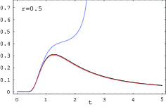
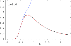
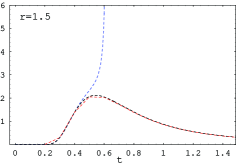
Figure 3 compares the approximation $\hat{\theta}(r,t)$ (black curves) against $\theta_{G}(r,t)$ (blue curves) and direct numerical integration (red curves). We note the same pattern of good agreement between $\hat{\theta}(r,t)$ and $\theta_{G}(r,t)$ at small $t$ , and increasing discrepancy for larger $t$ , which explodes to infinity for sufficiently large $t$ . The reason for this explosive behavior is the fact that the denominator in Eq. (74) approaches zero as $t$ approaches a certain maximum value. For $t$ larger than this value the denominator becomes negative and the approximation ceases to exist.

This maximum $t$ value is given by the inequality $u_{0}(t)<e^{-2-2\log(r/(2\sqrt{2}))}=\frac{8}{r^{2}e^{2}}$ . For $r=0.5$ this condition imposes the upper bound $t<t_{\rm max}=2.5538$ .

We show in Figure 4 plots of $\hat{\theta}(r,t)$ vs $t$ at $r=0.5,1.0,1.5$ . The vertical scale of the plot is chosen as in Figure 1 (left) of Bernhart and Mai [4], which shows the plots of $\theta(r,t)$ for the same parameters, obtained using a precise numerical inversion of the Laplace transform of $\theta(r,t)$ . The shapes of the curves are very similar with those shown in [4].

3.1. Asymptotics for $t\to 0$ and $t\to\infty$ of the approximation $\hat{\theta}(r,t)$

We study in this Section the asymptotics of the approximation $\hat{\theta}(r,t)$ defined in (73) for $t\to 0$ and $t\to\infty$ , and compare with the exact asymptotics of $\theta(r,t)$ in these limits obtained by Barrieu et al [3] and Gerhold [12].

As expected, the $t\to 0$ asymptotics matches precisely the exact asymptotics of $\theta(r,t)$ . Although the approximation $\hat{\theta}(r,t)$ was derived in the small $t$ limit, it is somewhat surprising that it matches also the correct asymptotics of $\theta(r,t)$ for $t\to\infty$ , up to a multiplicative coefficient, which however becomes exact as $r\to\infty$ .

Small $t$ asymptotics $t\to 0$ . The leading asymptotics of $\theta(r,t)$ as $t\to 0$ was obtained in Barrieu et al [3]

(76)

\theta(r,t)\sim e^{-\frac{1}{2t}\log^{2}t}\,.

This was refined further by Gerhold as in Eq. (74). Using the small $t$ approximation $u_{0}(t)=\frac{1}{2t^{2}}\log^{2}(1/t)$ (see Eq. (6) in Gerhold’s paper), the improved expansion (74) gives

(77)

\theta_{G}(r,t)\sim\frac{\log(1/t)}{t}\frac{1}{\sqrt{2\log\log(1/t)+2\log(2/t)}}e^{-\frac{1}{2t}\log^{2}(1/t)}\,.

The $t\to 0$ expansion of $\hat{\theta}(r,t)$ can be obtained using the $\rho\to 0$ asymptotics of $F(\rho),G(\rho)$ in points (i) of the Propositions 4 and 5, respectively. This gives

(78)

\hat{\theta}(r,t)\sim\frac{1}{t}\sqrt{\log 1/(rt)}e^{-\frac{1}{2t}\log^{2}(rt)-\frac{1}{t}\log(1/(rt))\log(2\log(1/(rt))+\frac{1}{t}\log(1/(rt))}\,,\quad t\to 0

The exponential factor agrees with the asymptotics of the exact result. Also the leading dependence of the multiplying factor reproduces the improved expansion following from [12].

Large $t$ asymptotics $t\to\infty$ . The $t\to\infty$ asymptotics of $\theta(r,t)$ is given in Remark 3 in Barrieu et al [3] as

(79)

\theta(r,t)\sim c_{r}\frac{1}{t^{3/2}}\,,\quad c_{r}=\frac{1}{\sqrt{2\pi}}K_{0}(r)\,.

The large $t$ asymptotics of $\hat{\theta}(r,t)$ is related to the $\rho\to\infty$ asymptotics of $F(\rho),G(\rho)$ . As $\rho\to\infty$ we have $F(\rho)\sim\rho$ from Prop. 4 point (ii) and $G(\rho)\sim\frac{\pi\rho}{(1+\rho)^{3/2}}$ from Prop. 5 point (ii). Substituting into (73) and keeping only the leading contributions as $t\to\infty$ gives

(80)

\hat{\theta}(r,t)\sim\frac{r}{2(1+rt)^{3/2}}e^{-r}\sim\frac{1}{2\sqrt{r}}t^{-3/2}e^{-r}\,.

The $t$ dependence has the same form as the exact asymptotics (79).

Let us examine also the coefficient of $t^{-3/2}$ in (80) and compare with the exact result for $c_{r}$ in (79). The leading asymptotics of the $K_{0}(x)$ function for $x\to\infty$ is $K(x)=e^{-x}\sqrt{\frac{\pi}{2x}}(1+O(1/x))$ . The exact coefficient becomes, for $r\to\infty$

(81)

c_{r}=\frac{1}{2}\frac{1}{\sqrt{r}}e^{-r}+O(1/r)

The leading term in this expansion matches precisely the coefficient obtained from $\hat{\theta}(r,t)$ . We conclude that the right tail asymptotics of $\hat{\theta}(r,t)$ approaches the same form as the exact asymptotics in the limit $r\to\infty$ .

4. Application: The asymptotic distribution of $\frac{1}{t}A_{t}^{(\mu)}$

As an application of the result of Proposition 1, we give here the leading $t\to 0$ asymptotics of the distribution of the time average of the gBM $\frac{1}{t}A_{t}^{(\mu)}$ .

The distribution of $\frac{1}{t}A_{t}^{(\mu)}$ can be obtained from Yor’s formula (3) by integration over $x$ . Introducing a new variable $u=at$ this is expressed as the integral

(82)

\mathbb{P}\left(\frac{1}{t}A_{t}^{(\mu)}\in da\right)=\int_{x\in\mathbb{R}}e^{\mu x-\frac{1}{2}\mu^{2}t}\exp\left(-\frac{1+e^{2x}}{2at}\right)\theta\left(\frac{e^{x}}{at},t\right)\frac{dadx}{a}\,.

Changing the $x$ integration variable to $x=\log(a\rho)$ , the range of integration for $x:(-\infty,\infty)$ is mapped to $\rho:(0,\infty)$ .

(83)

\displaystyle\mathbb{P}\left(\frac{1}{t}A_{t}^{(\mu)}\in da\right)=e^{-\frac{1}{2}\mu^{2}t}\frac{da}{a}\int_{0}^{\infty}(a\rho)^{\mu}e^{-\frac{1+a^{2}\rho^{2}}{2at}}\theta\left(\frac{\rho}{t},t\right)\frac{d\rho}{\rho}\,.

We would like to use here the asymptotic expansion for $\theta(\rho/t,t)$ from Proposition 1. Integrating term by term the asymptotic expansion requires a uniform bound on the approximation error. Such a bound was given in (53) based on numerical evidence, which is furthermore uniform in $\rho$ . Using this result one can transfer the asymptotic expansion of Proposition 1 to an asymptotic result for the density of the time-average of the gBM. Define this density as

\mathbb{P}\left(\frac{1}{t}A_{t}^{(\mu)}\in da\right)=f(a,t)\frac{da}{a}\,.

Proposition 6.

Assume the error bound (53). Then we have

(84)

f(a,t)=\frac{1}{2\pi t}e^{-\frac{1}{2}\mu^{2}t}\int_{0}^{\infty}(a\rho)^{\mu}e^{-\frac{1}{t}H(\rho)}G(\rho)\frac{d\rho}{\rho}\cdot(1+\varepsilon(a,t))

with

(85)

H(\rho):=\frac{1+a^{2}\rho^{2}}{2a}-\frac{\pi^{2}}{2}+F(\rho)\,.

The error term is bounded as $|\varepsilon(a,t)|\leq\frac{1}{70}t$ .

Furthermore, the density $f(a,t)$ has the asymptotic form in the small-maturity limit

(86)

f(a,t)\sim\frac{1}{\sqrt{2\pi t}}g(a,\mu)e^{-\frac{1}{t}J(a)}\,,\quad t\to 0\,,

with $J(a)\equiv\inf_{\rho\geq 0}H(\rho)=H(\rho_{*})$ and

(87)

g(a,\mu):=(a\rho_{*})^{\mu}G(\rho_{*})\frac{1}{\rho_{*}\sqrt{H^{\prime\prime}(\rho_{*})}}\,,\quad\rho_{*}=\arg\inf_{\rho}H(\rho)\,.

Proof.

The function $\theta(\rho,t)$ can be expressed as the leading order asymptotic term in Proposition 1

(88)

\theta(\rho/t,t)=\frac{1}{2\pi t}e^{-\frac{1}{t}(F(\rho)-\frac{\pi^{2}}{2})}G(\rho)\Big{(}1+\vartheta(\rho,t)\Big{)}\,,

where the error term $\vartheta(\rho,t)$ is bounded as in (53).

Substituting into the integral in (83) gives

(89)

\displaystyle\int_{0}^{\infty}(a\rho)^{\mu}e^{-\frac{1+a^{2}\rho^{2}}{2at}}\theta\left(\frac{\rho}{t},t\right)\frac{d\rho}{\rho}=\frac{1}{2\pi t}\int_{0}^{\infty}(a\rho)^{\mu}e^{-\frac{1}{t}H(\rho)}G(\rho)\frac{d\rho}{\rho}+I_{\varepsilon}(a,t)

with $\rho_{*}=\arg\inf_{\rho}H(\rho)$ .

The term $I_{\varepsilon}(a,t)$ is bounded using the error bound (53)

(90)

\displaystyle|I_{\varepsilon}(a,t)|\leq\int_{0}^{\infty}(a\rho)^{\mu}e^{-\frac{1+a^{2}\rho^{2}}{2at}}\hat{\theta}(\rho,t)|\vartheta(\rho,t)|\frac{d\rho}{\rho}\leq\frac{1}{70}t\int_{0}^{\infty}(a\rho)^{\mu}e^{-\frac{1+a^{2}\rho^{2}}{2at}}\hat{\theta}(\rho,t)\frac{d\rho}{\rho}

which gives $|\varepsilon(t)|\leq\frac{1}{70}t$ , as stated.

The asymptotic result (86) follows by application of the Laplace asymptotic expansion [11] to the integral (84). ∎

4.1. Properties of $J(a)$

In this section we give a more explicit result for the exponential factor $J(a)$ in the leading asymptotic density (84), and study its properties.

Proposition 7.

The function $J(a)$ is given by:

i) for $a\geq 1$ we have

(91)

\displaystyle J(a)=\frac{1}{2a}-\frac{1}{2a}\cosh^{2}x_{1}+\frac{1}{2}x_{1}^{2}=\frac{1}{2}x_{1}^{2}-\frac{1}{2}x_{1}\tanh x_{1}

where $x_{1}$ is the solution of the equation

(92)

\frac{\sinh 2x_{1}}{2x_{1}}=a\,.

This case corresponds to $0<\rho_{*}\leq 1$ .

ii) for $0<a\leq 1$ we have

(93)

J(a)=\frac{1}{2}(y_{1}-\pi)\tan(y_{1}-\pi)-\frac{1}{2}(y_{1}-\pi)^{2}

where $y_{1}$ is the solution of the equation

(94)

y_{1}-\frac{1}{a}\sin y_{1}\cos y_{1}=\pi\,.

This case corresponds to $1\leq\rho_{*}<\frac{\pi}{2}$ .

Proof.

We start with the expression

	$\displaystyle J(a)$	$\displaystyle=$	$\displaystyle\inf_{\rho\geq 0}\left(\frac{1+a^{2}\rho^{2}}{2a}-\frac{\pi^{2}}{2}+F(\rho)\right)$
		$\displaystyle=$	$\displaystyle\frac{1}{2a}+\frac{a}{2}\rho_{}^{2}-\frac{\pi^{2}}{2}+F(\rho_{})$

where $\rho_{*}$ is the solution of the equation

(96)

F^{\prime}(\rho)+a\rho=0\,.

Using the explicit result for $F^{\prime}(\rho)$ in Eq. (58) we get $F^{\prime}(\rho)<0$ for $0<\rho<\frac{\pi}{2}$ and $F^{\prime}(\rho)>0$ for $\rho>\frac{\pi}{2}$ . This implies that the solution of the equation (96) must satisfy $\rho_{*}\leq\frac{\pi}{2}$ . As $a\to 0$ the minimizer approaches the upper boundary $\lim_{a\to 0}\rho_{*}=\frac{\pi}{2}$ as $F^{\prime}(\frac{\pi}{2})=0$ .

The solution of (96) for $a=1$ is $\rho_{*}=1$ , since $F^{\prime}(1)=-1$ , from Prop. 4 point (iii).

The strategy of the proof is to eliminate $\rho_{*}$ using (58) in terms of $x_{1}$ and $y_{1}$ , respectively. Substituting (58) into (96) gives

(97)		$\displaystyle 0<\rho<1$	$\displaystyle:$	$\displaystyle\cosh x_{1}=a\rho$
(98)		$\displaystyle\rho>1$	$\displaystyle:$	$\displaystyle\cos y_{1}=-a\rho\,.$

These equations can be used to eliminate $\rho_{*}$ from the expression of $F(\rho_{*})$ . Substituting into (4.1) reproduces the results shown.

The function $\rho_{*}(a)$ has the expansion around $a=1$

(99)

\rho_{*}(a)=1-\frac{1}{4}(a-1)+\frac{19}{160}(a-1)^{2}-\frac{1511}{22400}(a-1)^{3}+O((a-1)^{4})\,.

To prove this expansion, assume first $a\to 1$ from above, and thus $\rho_{*}<1$ . From Eq. (97) it follows that

(100)

\rho_{*}=\frac{1}{a}\cosh x_{1}(a)

where $x_{1}(a)$ is the solution of $\frac{\sinh 2x_{1}}{2x_{1}}=a$ . Expanding around $a=1$ gives $x_{1}(a)=\sqrt{\frac{3}{2}(a-1)}+\cdots$ , and substituting above gives the expansion of $\rho_{*}(a)$ . A similar result is obtained by assuming $a\to 1$ from below.

∎

The function $J(a)$ has the following properties:

i) The function $J(a)$ vanishes at $a=1$ . The infimum in (4.1) is reached at $\rho_{*}=1$ .

ii) For $a>1$ the infimum is reached at $0<\rho_{*}<1$ . As $a\to\infty$ we have $\lim_{a\to\infty}\rho_{*}=0$ .

iii) For $0<a<1$ the infimum is reached at $1<\rho_{*}<\rho_{0}=\frac{\pi}{2}$ . As $a\to 0$ we have $\lim_{a\to 0}\rho_{*}=\pi/2$ .

4.2. Comparison with the Large Deviations result

The distributional properties of $A_{t}^{(\mu)}$ as $t\to 0$ were studied using probabilistic methods from Large Deviations theory in [2, 21, 23]. Assuming that $S_{t}$ follows a one-dimensional diffusion $dS_{t}=\sigma(S_{t})S_{t}dW_{t}+(r-q)S_{t}dt$ , it has been shown in [21] that, under weak assumptions on $\sigma(\cdot)$ , $\mathbb{P}\left(\frac{A_{t}}{t}\in\cdot\right)$ satisfies a Large Deviations property as $t\to 0$ . This result includes as a limiting case the geometric Brownian motion corresponding to $\sigma(x)=\sigma$ .

The main result can be extracted from the proof of Theorem 2 in [21], and can be formulated as follows.

Proposition 8.

Assume $S_{t}=e^{\sigma W_{t}+(r-\frac{1}{2}\sigma^{2})t}$ and $A_{t}=\int_{0}^{t}S_{t}dt$ . The time average of $S_{t}$ satisfies a Large Deviations property in the $t\to 0$ limit

(101)

\lim_{t\to 0}t\log\mathbb{P}\left(\frac{A_{t}}{t}\in\cdot\right)=-\frac{1}{\sigma^{2}}\mathcal{J}_{\rm BS}(\cdot)

with rate function $\mathcal{J}_{\rm BS}(\cdot)$ expressed as the solution of a variational problem, which is furthermore solved in closed form in Proposition 12 of [21].

The asymptotic density (84) has the same form as the exponential decay predicted by Large Deviations theory (101). We show here that the result for $J(a)$ in Proposition 7 is related to the rate function $\mathcal{J}_{\rm BS}(a)$ derived in [21] as

(102)

J(a)=\frac{1}{4}\mathcal{J}_{\rm BS}(a)\,.

The factor of 1/4 is due to the factor of 2 in the exponent of the definition of $A_{t}$ in the Yor formula (3), which acts as a volatility $\sigma=2$ .

The function $\mathcal{J}_{\rm BS}(x)$ is given by Proposition 12 in [21] which we reproduce here for convenience.

Proposition 9 (Prop. 12 in [21]).

The rate function $\mathcal{J}_{\rm BS}(x)$ is given by

(105)

\displaystyle\mathcal{J}_{\rm BS}(x)=\left\{\begin{array}[]{cc}\frac{1}{2}\beta^{2}-\beta\tanh\left(\frac{\beta}{2}\right)\,,&x\geq 1\\ 2\xi(\tan\xi-\xi)\,,&x\leq 1\\ \end{array}\right.

where $\beta$ is the solution of the equation

(106)

\frac{\sinh\beta}{\beta}=x

and $\xi$ is the solution in $[0,\pi/2]$ of the equation

(107)

\frac{\sin 2\xi}{2\xi}=x\,.

The relation (102) follows by identifying $x_{1}=\frac{1}{2}\beta$ in the first case of Proposition 7, and $y_{1}-\pi=\xi$ in the second case.

The rate function $\mathcal{J}_{\rm BS}(a)$ for $a\simeq 1$ can be expanded in a Taylor series in $\log a$ (see Eq. (36) of [21])

(108)

\mathcal{J}_{\rm BS}(a)=\frac{3}{2}\log^{2}a-\frac{3}{10}\log^{3}a+\frac{109}{1400}\log^{4}a+O(\log^{5}a)\,.

This expansion is convenient for numerical evaluation of the rate function. Proposition 13 in [21] gives also asymptotic expansions of $\mathcal{J}_{\rm BS}(a)$ for $a\to 0$ and $a\to\infty$ , which can be translated directly into corresponding asymptotic expansions for $J(a)$ .

4.3. Properties of $g(a,\mu)$

We study here in more detail the properties of the function $g(a,\mu)$ defined in (87). This can be put into a more explicit form as follows.

Proposition 10.

The function $g(a,\mu)$ has the explicit form

(109)

\displaystyle g(a,\mu)

\displaystyle=

\displaystyle e^{\mu\log a+(\mu-1)\log\rho_{*}(a)}G(\rho_{*})\frac{1}{\sqrt{H^{\prime\prime}(\rho_{*})}}=\frac{\sqrt{3}}{2}e^{c_{1}\log a+c_{2}\log^{2}a+O(\log^{3}a)}\,.

with

(110)		$\displaystyle c_{1}=\frac{3}{4}(\mu+1)-\frac{4}{5}$
(111)		$\displaystyle c_{2}=-\frac{3}{80}(\mu+1)+\frac{57}{1400}\,.$

Proof.

The proof follows by combining the expansions around $a=1$ of the factors in this expression:

i) $\rho_{*}(a)$ is given by (99) which is written in equivalent form as

(112)

\log\rho_{*}(a)=-\frac{1}{4}\log a-\frac{3}{80}\log^{2}a+\frac{1}{350}\log^{3}a+O(\log^{4}a)\,.

ii) $G(\rho_{*})$ is obtained by substituting the expansion of $\rho_{*}(a)$ into the expansion of $G(\rho)$ in powers of $\rho-1$ from Proposition 5

	$\displaystyle G(\rho_{*}(a))$	$\displaystyle=$	$\displaystyle\sqrt{3}\left(1+\frac{1}{20}\log a+\frac{37}{5600}\log^{2}a-\frac{41}{48000}\log^{3}a+O(\log^{4}a)\right)$
		$\displaystyle=$	$\displaystyle\sqrt{3}\exp\left(\frac{1}{20}\log a+\frac{3}{560}\log^{2}a-\frac{1}{875}\log^{3}a+O(\log^{4}a)\right)$

iii) $H^{\prime\prime}(\rho_{*}(a))=F^{\prime\prime}(\rho_{*}(a))+a$ can be evaluated using the expansion of $F(\rho)$ from Prop. 4 (iii) which gives

(114)

F^{\prime\prime}(\rho_{*})=3+\frac{9}{5}(a-1)-\frac{18}{175}(a-1)^{2}+O((a-1)^{3})\,.

We get

(115)

H^{\prime\prime}(\rho_{*}(a))=4+\frac{14}{5}(a-1)-\frac{18}{175}(a-1)^{2}+O((a-1)^{3})\,.

It is convenient to express this in terms of $\log a$ as

(116)

H^{\prime\prime}(\rho_{*})=4\exp\left(\frac{7}{10}\log a+\frac{111}{1400}\log^{2}a+O(\log^{3}a)\right)\,.

∎

Remark 11.

We have $g(1,\mu)=\frac{\sqrt{3}}{2}$ for all $\mu\in\mathbb{R}$ . This follows by noting that at $a=1$ we have $\rho_{*}(1)=1$ , and thus the only factors different from 1 are $G(1)=\sqrt{3}$ and $H^{\prime\prime}(1)=4$ .

Numerical evaluation of the function $g(a,\mu)$ shows that for the driftless gBM case $\mu=-1$ this function is decreasing in $a$ , and becomes increasing for sufficiently large and positive $\mu$ .

Acknowledgements

I am grateful to Peter Nándori and Lingjiong Zhu for very useful discussions and comments.

Appendix A Subleading correction

We give here the subleading correction to the asymptotic expansion of the Hartman-Watson integral $\theta(\rho/t,t)$ in Proposition 1.

The first two terms of the asymptotic expansion of the Hartman-Watson integral as $t\to 0$ are

(117)

\theta(\rho/t,t)=\frac{1}{2\pi t}G(\rho)e^{-\frac{1}{t}(F(\rho)-\frac{\pi^{2}}{2})}\left(1+\frac{1}{2}t\tilde{g}_{2}(\rho)+O(t^{2})\right)

where

(120)

\displaystyle\tilde{g}_{2}(\rho)=\left\{\begin{array}[]{cc}\frac{-12+9\rho\cosh x_{1}-2\rho^{2}\cosh^{2}x_{1}+5\rho^{2}}{12(\rho\cosh x_{1}-1)^{3}}&\,,0<\rho\leq 1\\ \frac{12+9\rho\cos y_{1}+2\rho^{2}\cos^{2}y_{1}-5\rho^{2}}{12(1+\rho\cos y_{1})^{3}}&\,,\rho>1\\ \end{array}\right.

The result follows straighforwardly by keeping the next terms in the expansions of the integrals appearing in the proof of Proposition 1.

The plot of $\tilde{g}_{2}(\rho)$ is given in the left panel of Figure 5. It reaches a maximum (in absolute value) at $\rho=1$ where it is equal to $\tilde{g}_{2}(1)=-\frac{1}{35}$ .

We list next a few properties of the function $\tilde{g}_{2}(\rho)$ . This function has the expansion around $\rho=1$

(121)

\tilde{g}_{2}(\rho)=-\frac{1}{35}+\frac{144}{67375}(1/\rho-1)+O((1/\rho-1)^{2})\,.

As $\rho\to\infty$ we get, using the asymptotics of $y_{1}\to 0$ from the proof of Prop. 4(ii),

(122)

\tilde{g}_{2}(\rho)=-\frac{1}{4\rho}+\frac{3}{2\rho^{2}}+O(\rho^{-3})\,.

For $\rho\to 0$ , recall from the proof of Proposition 4 (i) that $\rho\cosh x_{1}\sim\log(1/\rho)\to\infty$ , which gives the asymptotics

(123)

\tilde{g}_{2}(\rho)=-\frac{1}{6}\frac{1}{\log(1/\rho)}+O(\log^{-2}(1/\rho))\,.

References

[1] A. Antonov, M. Konikov and M. Spector, Modern SABR Analytics. Springer, New York, 2019.
[2] L.P. Arguin, N.-L. Liu and T.-H. Wang. (2018) Most-likely-path in Asian option pricing under local volatility models. International Journal of Theoretical and Applied Finance. 21, 1850029.
[3] P. Barrieu, A. Rouault and M. Yor, A study of the Hartman-Watson distribution motivated by numerical problems related to the pricing of Asian options, J. Appl. Probab. 41, 1049-1058 (2004)
[4] G. Bernhart and J.-F. Mai, A note on the numerical evaluation of the Hartman-Watson density and distribution function, in Innovations in Quantitative Risk Management, p.337, K. Blau, M. Scherer and R. Zagst (Eds.), Springer Proceedings in Mathematics and Statistics, Springer, 2015.
[5] P. Boyle and A. Potapchik, Prices and sensitivities of Asian options: A survey. Insurance: Mathematics and Economics 42, 189-211 (2008)
[6] N. Cai, Y. Song and N. Chen, Exact simulation of the SABR model, Operations Research 65(4), 931-951 (2017)
[7] A. Comtet, C. Monthus and M. Yor, Exponential functionals of Brownian motion and disordered systems. J. Appl. Probab. 35, 255 (1998)
[8] D. Dufresne, Laguerre series for Asian and other options, Math. Finance 10, 407-428 (2000)
[9] D. Dufresne, The integral of the geometric Brownian motion, Adv. Appl. Probab. 33, 223-241 (2001).
[10] D. Dufresne, Bessel processes and a functional of Brownian motion, in M. Michele and H. Ben-Ameur (Eds.), Numerical Methods in Finance 35-57, Springer, 2005.
[11] A. Erdélyi, Asymptotic expansions, Dover Publications 1956
[12] S. Gerhold, The Hartman-Watson distribution revisited: asymptotics for pricing Asian options, J. Appl. Probab. 48(3), 892-899 (2011).
[13] A. Gulisashvili and E.M. Stein, Asymptotic behavior of the distribution of the stock price in models with stochastic volatility: the Hull-White model, C.R. Math. Acad. Sci. Paris 343, 519-523 (2006)
[14] A. Gulisashvili and E.M. Stein, Asymptotic behaviour of distribution densities in models with stochastic volatility. I. Math. Finance 20, 447-477 (2010)
[15] P. Hartman and G.S. Watson, ”Normal” distribution functions on spheres and the modified Bessel functions, Ann. Probab. 2, 593-607 (1974)
[16] K. Ishyiama, Methods for evaluating density functions of exponential functionals represented as integrals of geometric Brownian motion, Methodol. Comput. Appl. Probab. 7, 271-283 (2005)
[17] J.T. Kent, The spectral decomposition of a diffusion hitting time, Ann. Probab. 10(1), 207-219 (1982).
[18] H. Matsumoto and M. Yor, On Dufresne’s relation between the probability laws of exponential functionals of Brownian motions with different drifts, Adv. Appl. Probab. 35, 184-206 (2003)
[19] H. Matsumoto and M. Yor, Exponential functionals of Brownian motion: I. Probability laws at fixed time, Prob. Surveys 2, 312-347 (2005)
[20] F.W.J. Olver, Introduction to asymptotics and special functions, Academic Press 1974.
[21] D. Pirjol, L. Zhu, Short maturity Asian options in local volatility models, SIAM J. Finan. Math. 7(1), 947-992 (2016); arXiv:1609.07559[q-fin].
[22] D. Pirjol, L. Zhu, Asymptotics for the discrete-time average of the geometric Brownian motion, Adv. Appl. Probab. 49, 1-53 (2017)
[23] Pirjol, D. and L. Zhu. (2017). Short maturity Asian options for the CEV model, Probab. Eng. Inform. Sc. 33(2), 258-290, 2019. arXiv:1702.03382 [q-fin.PR]
[24] M. Schröder, On the integral of the geometric Brownian motion, Adv. Appl. Probab. 35, 159-183 (2003)
[25] M. Yor, On some exponential functionals of Brownian motion, Adv. Appl. Probab. 24, 509-531 (1992)

Asymptotic expansion for the Hartman-Watson distribution

Abstract.

Key words and phrases:

1. Introduction

2. Asymptotic expansion of θ​(ρ/t,t)\theta(\rho/t,t) as t→0t\to 0

Proposition 1.

Proof of Proposition 1.

Remark 2.

2.1. Error estimates

Remark 3.

Proof.

2.2. Properties of the functions F​(ρ)F(\rho) and G​(ρ)G(\rho)

Proposition 4.

Proof.

Proposition 5.

Proof.

3. Numerical tests

3.1. Asymptotics for t→0t\to 0 and t→∞t\to\infty of the approximation θ^​(r,t)\hat{\theta}(r,t)

4. Application: The asymptotic distribution of 1t​At(μ)\frac{1}{t}A_{t}^{(\mu)}

Proposition 6.

Proof.

4.1. Properties of J​(a)J(a)

Proposition 7.

Proof.

4.2. Comparison with the Large Deviations result

Proposition 8.

Proposition 9 (Prop. 12 in [21]).

4.3. Properties of g​(a,μ)g(a,\mu)

Proposition 10.

Proof.

Remark 11.

Appendix A Subleading correction

References

2. Asymptotic expansion of $\theta(\rho/t,t)$ as $t\to 0$

2.2. Properties of the functions $F(\rho)$ and $G(\rho)$

3.1. Asymptotics for $t\to 0$ and $t\to\infty$ of the approximation $\hat{\theta}(r,t)$

4. Application: The asymptotic distribution of $\frac{1}{t}A_{t}^{(\mu)}$

4.1. Properties of $J(a)$

4.3. Properties of $g(a,\mu)$