Asymmetry activation and its relation to coherence under permutation operation
Abstract
A Dicke state and its decohered state are invariant for permutation. However, when another qubits state to each of them is attached, the whole state is not invariant for permutation, and has a certain asymmetry for permutation. The amount of asymmetry can be measured by the number of distinguishable states under the group action or the mutual information. Generally, the amount of asymmetry of the whole state is larger than the amount of asymmetry of the added state. That is, the asymmetry activation happens in this case. This paper investigates the amount of the asymmetry activation under Dicke states. To address the asymmetry activation asymptotically, we introduce a new type of central limit theorem by using several formulas on hypergeometric functions. We reveal that the amounts of the asymmetry and the asymmetry activation with a Dicke state have a strictly larger order than those with the decohered state in a specific type of the limit.
1 Introduction
Asymmetry is a root of the variety of various physical phenomena. Consider a perfectly symmetric state. Such a state does not reflect any changes so that it can realize no variety. To realize rich variety, the state needs to have sufficient asymmetry. In physics, people consider that symmetry breaking is needed for our world. Therefore, to explain various phenomena, many researchers introduced spontaneous symmetry breaking, which plays an important role in various areas in physics, nuclear star, superfluidity, superconductivity, cold atoms, Higgs boson, Nambu-goldstone boson. When the degree of symmetry breaking is large, it realizes rich phenomena. Since the amount of symmetry breaking can be restated as the amount of asymmetry, it is a central topic to study the amount of asymmetry.
Fortunately, quantum information theory has strong tools to evaluate the amount of asymmetry [1, 2]. The variety generated by group symmetry under a given state can be measured by the number of distinguishable states generated by group action to describe the symmetry. This number is evaluated by the difference between the von Neumann entropy of the averaged state with respect to the group action and the von Neumann entropy of the original state. This fact can be shown by a simple application of quantum channel coding theorem [3, 4] to the family of the states translated by the group action although this idea can be backed to various studies [5, 6, 7]. Therefore, the difference between the von Neumann entropies of these two states can be considered as the amount of the asymmetry of the given state. Now, we focus on the permutation symmetry on qubits similar to the recent paper [8]. When we apply the permutation of the state , the averaged state is permutation-invariant, and has no asymmetry. However, it still works as a resource for asymmetry when it is attached to another qubits state . When we have only the state , the amount of asymmetry is measured by the von Neumann entropy of . When the state is attached, the amount of asymmetry is , which is larger than the asymmetry of the added state. In this paper, we focus on the increase of the amount of asymmetry by adding an invariant state, and call this phenomena an asymmetry activation. In fact, an asymmetry activation with various groups often happens behind of symmetry breaking. In this paper, we study the asymmetry activation under quantum information-theoretical objects because no systematic research studied the asymmetry activation in the area of quantum information.
Now, we discuss how quantum theory can improve the asymmetry activation because the above state is classical. To address this problem, we focus on the coherence, which is a key concept in quantum theory [9]. That is, we consider a permutation-invariant state with great coherence. We focus on the Dicke state with the same weight as the classical state . This state has the largest coherence among invariant states with the same weight as the state because any invariant state with the same weight has the same diagonal elements as the state . A Dicke state has been playing an important role in the calculation of entanglement measures [10, 11, 12, 13, 14], quantum communication, and quantum networking [15, 16]. The experiments [15, 16] are motivated by the fact the overlap of symmetric Dicke states with biseparable states is close to 1/2 for large [17]. Multipartite entanglement has been detected in an ensemble of thousand of atoms realizing a Dicke state [18]. Some typical Dicke states have been realized in trapped atomic ions [19]. Recently, the multi-qubit Dicke state with half-excitations has been employed to implement a scalable quantum search based on Grover’s algorithm by using adiabatic techniques [20]. These studies show the importance of Dicke states
In particular, the Dicke state can be used for quantum metrology, which has been tested experimentally in cold gases of thousands of atoms [21, 22]. The Dicke states are optimal in linear interferometers, in the sense, that they saturate the inequality , which are saturated also by GHZ states [23, 24]. Here, is the quantum Fisher information corresponding to a unitary dynamics. Also the reference [25] studied the estimation of the same direction with Dicke states. These studies consider the information only for the direction of the rotation by the special unitary group. They do not focus on the direction of permutation because the Dicke state is invariant for permutation. It is a completely new idea to use the information of the direction of permutation by modifying the Dicke state. To execute this new idea, using non-negative integers as , , we consider the asymmetry of the following state.
| (1) |
The amount of asymmetry is the von Neumann entropy , where expresses the averaged state with respect to the permutation.
However, the calculation of this von Neumann entropy is not simple while is calculated to , which is approximated to , where is the binary entropy. This calculation is closely related to Schur-Weyl duality, one of the key structure in the representation theory. When we make a measurement given by the decomposition defined by Schur-Weyl duality for the system whose state is , we obtain the distribution of this measurement outcome. This distribution takes a key role in this calculation, The paper [26] discovered notable formulas for this distribution by using Hahn and Racah polynomials, which are - and -hypergeometric orthogonal polynomials, respectively. It is possible to numerically calculate this von Neumann entropy by using these tools.
Even though its numerical calculation is possible, it is quite difficult to understand its behavior. To grasp its trend, we consider two kinds of asymptotics, i.e., Type I and Type II limits. Type I limit assumes that and are fixed and is linear for , i.e., with fixed ratio , under . Type II limit does that and are linear for under . Type I limit corresponds to the situation of the law of small numbers, and Type II limit corresponds to the situation of the central limit theorem. For the relation of Type I and Type II limits with the law of small numbers and the central limit theorem, see Appendix A. Based on these formulas, the paper [27] derived the asymptotic approximation of the distribution in the limit .
In Type I limit, we show that the von Neumann entropy behaves as
| (2) | ||||
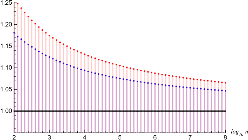
The same scaling appears in the bosonic coherent channel when the total power is fixed and the number of modes increases [28]. Figure 1 shows an example of this approximation. When we use the decohered state , the amount of asymmetry is calculated as
| (3) | ||||
The amount of asymmetry in (3) is a constant for while the case with Dicke state has the order as (2). In particular, in this scenario, while the size of the added system is finite, the amount of activated asymmetry goes to infinity. Therefore, the Dicke state significantly improves the amount of asymmetry over the decohered state under Type I limit.
In Type II limit, i.e., the limit with and linear for , we need to treat many ratios and parameters, which are summarized in Table 1. While the fixed ratios 1 and 2 are natural, the fixed ratio 3 is useful for our purpose.
| fixed ratio | , |
|---|---|
| set 1 | , |
| fixed ratio | , |
| set 2 | |
| fixed ratio | , |
| set 3 | |
| limit pdf | , |
| parameters |
Then, we show that
| (4) |
Since the amount of asymmetry of the added system is and is approximated to , the amount of the asymmetry activation is approximated to .
When we use the decohered state , the amount of asymmetry is calculated as
| (5) | ||||
Hence, the amount of the asymmetry activation is approximated to . For this derivation, we employ a kind of central limit theorem obtained in [27]. Since the inequality holds as shown later, the Dicke state significantly improves the amount of asymmetry over the decohered state even under Type II limit. In addition, similar characterization is also possible from the viewpoint of the number of distinguished states.
When the Dicke state is decohered, the state changes to the classical state . Since both states are invariant for permutation, their difference is the existence/non-existence of the coherence. Therefore, the difference between (2) and (3) and the difference between (4) and (5) can be considered as the improvement of asymmetry by using the coherence. In addition, the formula (4) has a very simple form and is characterized by the binary entropy of the quantity . Since the quantity has not appeared in physics, the formula (4) means that the quantity is a newly discovered quantity that has a physical role related to asymmetry. Therefore, we can expect that the new quantity takes certain roles in other topics.
The remaining part of this paper is organized as follows. As a preparation, Section 2.1 discusses the general theory for the amount of asymmetry, and prepares several formulas for the number of distinguished states. Also, it explains the general theory for asymmetry activation. Section 3 gives our problem setting, and introduces a key distribution to determine the amount of asymmetry. Section 4 discusses the amount of asymmetry for the decohered state. Section 5 reviews the asymptotic behavior of the distribution related to Schur-Weyl duality, which was obtained in the paper [27]. Section 6 derives the asymptotic behavior of the von Neumann entropy of the average state, which expresses the asymptotic behavior. Section 7 considers the asymptotic behavior of the number of distinguishable states. Section 8 gives another example for the asymmetry activation. Section 9 gives the conclusion and discussion.
Appendix B gives the proofs of the statements given in Section 3. Appendix C gives the derivation of the statement given in Section 4. Appendix D gives the derivation of the statements given in Sections 6 and 7. Appendix E shows an asymptotic formula for the von Neumann entropy presented in Section 6.
2 General theory
2.1 General theory for asymmetry
First, we discuss a general theory for asymmetry when a unitary representation of a finite group is given on . Since the invariance of a state under the -action is expressed as for any , the asymmetry of is considered as the degree of change caused by the -action. When a state is generated with equal probability , the averaged state with respect to the representation is given as
| (6) |
In this case, the map is considered as a classical-quantum channel, and the mutual information is given as
| (7) | ||||
where the von Neumann entropy is defined as . If we use the relative entropy , the mutual information is rewritten as
| (8) |
because . That is, the asymmetry is measured by . Therefore, the mutual information (7) can be considered as the degree of asymmetry of under the representation . This quantity was also introduced in the context of the resource theory of asymmetry [2] and other context [1]. In particular, when is a pure state , it is simplified to
| (9) |
Further, when a channel satisfies the covariance condition:
| (10) |
the information processing inequality for implies
| (11) |
This fact shows that the application of a covariant channel decreases the amount of asymmetry.
In fact, to connect the mutual information (7) and the distinguishability, we need to consider the repetitive use of the classical-quantum channel defined by . When our interest is the case when the above classical-quantum channel is used only once, we need to prepare another measure. In this case, we evaluate the number of distinguished states among with error probability .
Assume that the state is a constant times of a projection to a -dimensional subspace and the set is composed of orthogonal states. In this case is a constant times of a projection to a -dimensional subspace. In this case, the number of distinguishable state is . Also, equals . When we allow error probability with a positive integer , the number of distinguishable inputs is . This is because it is allowed that informations are represented to the same state. Hence, we have the formula
| (12) |
Next, we prepare a general formula for for a general state when the set of states is given. We prepare the following notation. Given a Hermitian matrix , the symbols and express the projections to the eigenspace of corresponding to non-negative and strictly positive eigenvalues, respectively. For two Hermitian matrices and , the symbol denotes the projection . Other projections such as and are similarly defined. Then, we consider the information spectrum relative entropy , which is given by [29]:
| (13) |
2.2 General theory for asymmetry activation
The asymmetry activation is generally formulated as follows. We consider two quantum systems and , and two unitary representation and of compact groups and on and , respectively. Then, we consider a larger compact group that contains and its unitary representation on , which satisfies . We choose an invariant state on and a state on . Then, the amount of asymmetry of the original state is . In contrast, the amount of asymmetry of the whole state is . Hence, the amount of the asymmetry activation is calculated as
| (19) |
Now, we choose a TP-CP map on and a TP-CP map on . When the covariance condition
| (20) |
holds for , the information processing inequality for implies
| (21) |
When the decoherence operator satisfies the above condition (20), the decoherence reduces the amount of the asymmetry activation.
3 Formulation
This paper investigates how an invariant state activates the amount of asymmetry. To address this question, we focus on the -fold tensor product of the qubit system , and consider it as the representation space of the permutation group acting by permutation of tensor factors as
| (22) |
Then, we apply the general theory given in Subsection 2.2 when , , , , and is defined as
| (23) |
while the state is asymmetric with respect to the permutation.
As one possible choice of , we choose a Dicke state on , which is a typical invariant state because it is given as the permutation invariant state with fixed weights and as
| (24) |
Remember that the state is defined as
| (25) |
In contrast, the decohered state of the Dicke state is given as
| (26) | ||||
To study the asymmetry, we focus on the - Schur-Weyl duality on the tensor product system depicted as
| (27) |
The Schur-Weyl duality claims that we have the following decomposition of into irreducible representations (irreps for short):
| (28) |
Here denotes the tensor product of linear spaces, equipped with -action on the left and -action on the right factor, denotes the -irrep corresponding to the partition , and denotes the highest weight -irrep of dimension . Using the hook formula (see [30, I.5, Example 2; I.7, (7.6)] for example), we can compute the dimension of as
| (29) | ||||
where denotes a box in the Young diagram corresponding to the partition . Using this formula, we have the completely mixed state . The highest weight -irrep of dimension has the standard basis , where and express the total and z-direction angular momenta, respectively.
In our analysis, the projector onto the isotypical component in the decomposition (28) plays a key role, and is defined as
| (30) |
As the set of the projectors forms a projective measurement, we define the probability as
| (31) |
and denote the corresponding probability distribution by . Since we can switch in the system, the probability mass function (pmf) enjoys the system symmetry
| (32) |
Since the distribution describes the averaged state as
| (33) | ||||
our analysis is concentrated in the distribution . We also denote by a discrete random variable distributed by the probability mass function (pmf for short) . We choose integers and from the following set;
| (34) | ||||
Then, the von Neumann entropy is given by
| (35) | ||||
which expresses the amount of asymmetry of . Furthermore, we can also consider the number of approximately orthogonal elements among the states , which is characterized by a slightly different quantity. As explained in Section 7, the number of distinguishable elements with error probability is approximated by the following value:
| (36) | ||||
4 Asymmetry with decohered symmetric state
First, we discuss the case with the decohered state . Then, we have
| (37) |
To consider the relation with , we consider the pinching map defined as
| (38) |
which expresses the decoherence process. Since the pinching map satisfies the covariance condition (10) with respect to permutation, the relation (11) yields the inequality
| (39) |
This inequality also follows from the inequality (21) for the amount of asymmetry activation. Therefore, the Dicke state realizes a larger amount of asymmetry than the decohered state. However, this inequality does not explain how much the Dicke state improves it over the decohered state. To answer this question, we need to consider the asymptotic behavior.
Here, we consider the number as well. Counting the possible combinatorics, we find that the number of discriminated states is calculated as . Since the set is composed of orthogonal states, due to (12), the difference between and with finite error probability is a constant. Hence, we discuss the asymptotics of the value given in (37).
5 Asymptotics analysis on distribution
To derive the asymptotic behaviors of and , we need the asymptotic analysis of our distribution under the limit . The paper [27] studied the following two cases.
-
1.
The limit with and fixed.
-
2.
The limit with , and fixed.
We call them Type I and II limits, respectively. The details are given in Subsection 5.1 and Subsections 5.2. Hereafter we denote by the probability for the distribution , and by a random variable distributed subject to the distribution. The contents of this section were already shown in the paper [27].
5.1 Asymptotic analysis of Type I limit
To address Type I limit, we employ the binomial distribution with trials with successful probability whose pmf is given by . Then, we introduce the distribution where denotes the convolution of probability distributions. Its pmf is denoted by and written as
| (42) | ||||
where and .
Theorem 1.
In the limit with and fixed, the distribution is approximated to the above-defined distribution up to . In particular, the asymptotic expectation is given by
| (43) |
In fact, it is known as the law of small numbers that the distribution converges to a Poisson distribution as goes to infinity with a fixed number . In Type I limit, and are fixed, and correspond to the fixed number of the law of small numbers. That is, we can consider Type I limit as the law of small numbers in our setting.
Remark 2.
Since the limit pmf is a convolution of two binomial distributions. it is a polynomial of , and this property was used in the paper [31].
5.2 Asymptotic analysis of type II limit
We discuss Type II limit. For this aim, we employ three kinds of parametrizations of the fixed ratios as Table 1. For example, the condition in (34) is equivalent to
| (44) |
However, in the following, we employ the set of three parameters , which are also free parameters under the conditions and . Also, the following quantities are fundamental for the discussion:
| (45) | ||||
These definitions of these parameters are summarized in Table 1.
Theorem 3.
Consider the limit with fixed ratios , , and . Then, for any , we have
| (46) |
In particular, the expectation behaves as
| (47) |
Considering the definition of the variance by using , we find the following fact. When the relation nor does not hold, i.e.,
| (48) |
the variance is well defined by (45) and is strictly positive. Then, we have the following theorem.
Theorem 4.
Assume the condition (48). Then, for any real , the relation
| (49) |
holds. In particular, the pmf behaves as
| (50) | ||||
In addition, we have
| (51) | |||
| (52) | |||
| (53) |
for
In the special case , we can further discuss the tight exponential evaluation of the tail probability as follows.
Proposition 5.
In Type II limit with , and , the probability goes to zero exponentially for any .
6 Asymptotics analysis on
As an interlude, let us derive the asymptotic formula (2) of for the state with respect to the distribution in Type I limit with fixed , and . We denote the pmf by , and the limit pmf by for simplicity. Thus, we have by Theorem 1. Now, recall the expression (35) of , which includes the dimension formula in (29). Let us cite from [32, Chap. 5, (5.12)] the asymptotic formula of binomial coefficient for fixed :
| (54) | ||||
Applying it to the dimension formula, we show (2) as
| (55) | ||||
where we used the asymptotic expectation in (43). The last line in (55) shows the conclusion (2). Therefore, with the comparison with (37) and (40), Dicke state significantly improves the amount of asymmetry over the classical symmetric state .
Continuing the interlude, we consider Type II limit of . When , i.e., , we have . Hence, we have
| (56) |
which was already discussed in Section 4. The same discussion can be applied to the case with . When , we have so that . In this case, is also zero. These cases have no difference from the case in Section 4. Therefore, we assume the assumption (48) in the following.
We have
| (57) | ||||
which is shown in Appendix D. Theorem 4 implies that
| (58) |
When the relation holds additionally, the relation (58) is replaced by a more precise form as follows
| (59) |
This relation will be shown in Proposition 14 in E, and the the precise form of the constant is given in Proposition 14.
Due to (37) and (41), the comparison between the Dicke state and the decohered state is summarized to the comparison between their first-order terms and . In fact, the limit in (39) with the division by implies
| (60) |
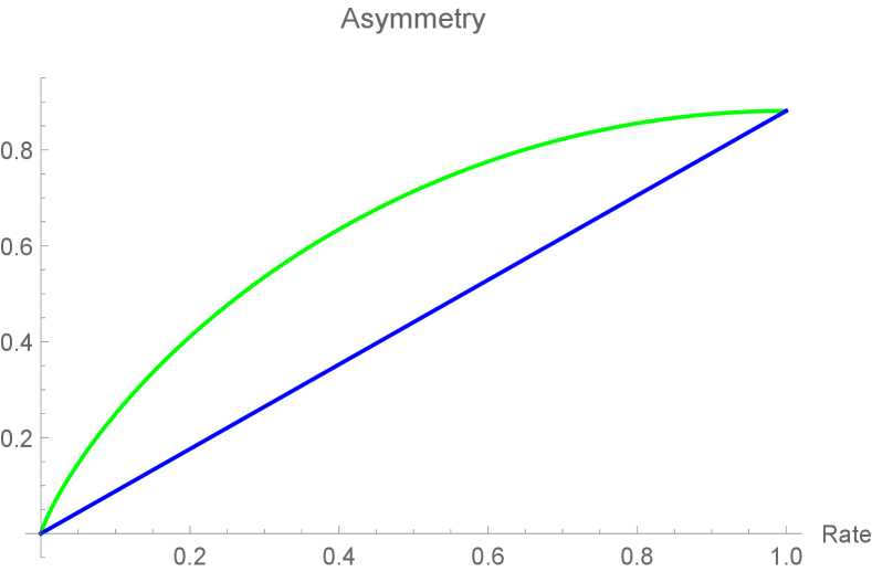
Here, we employ the relations (41) and (58). The difference between LHS and RHS shows the asymptotic difference of the amounts of the asymmetry activation caused by the decoherence. We consider the case when , in which two free parameters describe other parameters as
| (61) | ||||
Then, since and , we have
| (62) | ||||
In this case, and are plotted as Fig. 2.
7 Asymptotics analysis on
Next, to address the asymptotic behavior of , we apply the discussion in Section 2.1 to our setting. Since the state is characterized as (33), equals which is defined in (36). Hence,
| (63) | ||||
To discuss Type I limit, we denote the cdf of by . By recalling the dimension formula (29) of , is approximated to with a fixed value by (54). When is sufficiently large, is monotonically increasing for . We choose as . Hence, the combination of (63) and Theorem 1 implies
| (64) | ||||
The combination of (17), (18), and (64) yields
| (65) | ||||
8 Another example of asymmetry activation
To consider another simple example of asymmetry activation, we choose , , and the -tensor product representation of as , , and , respectively. Then, the -tensor anti-symmetric subspace of is a one-dimensional space. We choose the unique state on the -tensor anti-symmetric subspace of as the invariant state . Given , we choose , , and the -tensor product representation of as , , and , respectively.
We choose and the -tensor product representation of as and , respectively. We choose the state as a state on the anti-symmetric subspace of . Since the dimension of is , . In this case, the vector of the support of is invariant for the exchange of the first and second system. Hence, the vector of the support belongs to the symmetric subspace of , whose dimension is . Thus, we have . Therefore, the amount of the asymmetry activation is
| (69) |
Given a fixed integer , the amount of the asymmetry activation takes the maximum when . In this case, this value is approximated to be .
9 Conclusion and discussion
We have shown that the coherence in the Dicke state enhances the asymmetry for the permutation when a qubits state is attached. To clarify the merit of the coherence, we have discussed two types of limits, Type I and II limits. In these limits, the case with the Dicke state has a larger amount of degree than the case with the decohered state. In particular, under Type I limit, the amount of the degree in the former has a strictly larger order than that of the latter. Under Type II limit, both cases have different leading terms. Their difference characterizes the effect of the existence of the coherence. This fact shows the importance of the coherence even in the asymmetry and the asymmetry activation for permutation.
Here, we emphasize the generality of the concept of asymmetry activation. Asymmetry activation may happen in various situations. To explain this aspect, we have shown another example in Section 8. It is another interesting future study to discuss various examples of asymmetry activation.
Using this discussion, we have derived the inequality (60). Since the inequality (60) can be considered without this type of limit, it is possible to directly derive this inequality without considering this type of limit. This kind of derivation is an interesting future study. Further, our analysis has revealed the physical importance of the value , whose importance has not been recognized until this study.
For our asymptotic derivations, we have employed various asymptotic formulas for the distribution . Since the distribution has a highly complicated form, this fact shows the usefulness of these asymptotic formulas. Since the distribution is based on the the Schur-Weyl duality, which is a key structure in quantum information, we can expect that these formulas can be used in other topics in quantum information.
Appendix A Type I and Type II limits and Limit theorems for binomial distributions
First, we summarize existing results for binomial distributions. Given a real number , we define the binomial distribution as
| (70) |
The central limit theorem addresses the case when is fixed and increases. It states
| (71) |
However, the above convergence is not uniform when is close to or . To cover the asymptotic behavior in this case, we consider the case when is chosen to and increases. Then, we have the following relation
| (72) |
which is called the law of small numbers.
In our model, expresses the total number of and expresses the total number of . Hence, the ratio corresponds to the parameter in the binomial distribution. Hence, Type I and Type II limits corresponds to the law of small number and the central limit theorem, respectively. Therefore, although Type II limit works with , when is close to zero, Type II limit does not work so that Type I is needed for this case.
Appendix B Single-shot bounds for cq-channels
The aim of this section is to derive the inequalities (17) and (18), which will be shown in Theorem 9. We begin with a general setting of classical-quantum channel explained in Subsection 7.
B.1 Single-shot bound for general cq-channel
We consider a pure state channel where is a state on a Hilbert space . Let be the number of distinguished states among . We consider a joint system , where is a Hilbert space spanned by . Dependently of a distribution on and a state on , we define two states and on the joint system by
| (73) | ||||
and a state on by
| (74) |
Recall the information spectrum relative entropy in (13):
| (75) |
The hypothesis testing relative entropy is defined by [34]
| (76) | ||||
Nagaoka [35] essentially showed the following inequality for any channel.
Lemma 6.
For any state , we have
| (77) |
By [36, Corollary 1], we have the following inequality for any mixed state :
Lemma 7.
The inequality
| (78) |
holds.
Lemma 8.
The inequality
| (79) |
holds.
B.2 Single-shot bound for pure state channel
In the case when the states are pure states, we have the following theorem.
Theorem 9.
When all states are pure states, we have the following relations.
| (80) | ||||
| (81) |
To show Theorem 9, we prepare the following Lemmas 10 and 11, using the fact that is a pure state. Although these two lemmas were essentially proved in [28, Appendix II], it is difficult to extract them from the reference, and we present them here with proofs.
Lemma 10.
The relation
| (82) |
holds.
Proof.
We define the projection as
| (83) |
Hence, we have
| (84) |
and thus
| (85) |
Since the support of is included in the support of and is the zero matrix or a rank-one projection, is the zero matrix or a rank-one matrix whose eigenvalue is not greater than . Hence,
| (86) |
We define the projection as
| (87) |
Then, using (85) and (86), we have
∎
Lemma 11.
We have
| (88) |
Proof.
In this proof, we set . We choose and assume that
| (89) |
Proof of Theorem 9.
We will show Theorem 9 by combining Lemmas 10 and 11 to Lemmas in Appendix B.1. The inequality (80) is shown as follows:
| (98) | ||||
where steps , and follow from (78) of Lemma 7, from the second equation of (79) of Lemma 8, and from (88) of Lemma 11, respectively. The inequality (81) is shown as follows:
| (99) | ||||
In the step , we applied (77) of Lemma 6 to the case with . The steps and follow from the second inequality in (79) of Lemma 8, and from (82) of Lemma 10, respectively. ∎
B.3 Single-shot bound for pure state covariant channel
Now, we consider the group covariant case, i.e., the case when the set of states is given as , where is a finite group, is its unitary representation, and is a pure state. In this case, Theorem 9 is simplified as follows. The following theorem shows (17) and (18).
Theorem 12.
When is given as the above defined set , we have the following relations.
| (100) | ||||
| (101) |
Appendix C Derivations of (40) and (41)
Appendix D Derivations of (57) and (66)
We derive the formulas (57) and (66). In Type II limit, using (105), we obtain (57) as
| (109) |
where each step is derived as follows. follows from the relation , follows from the relation in (29). follows from the relation (105).
Next, we show (66). In Type II limit, to evaluate the value , we introduce the following quantities.
| (110) | ||||
| (111) |
We have
| (112) |
Also, we have
| (113) |
Thus,
| (114) |
Also, we denote by and the cdfs of the standard Gaussian distribution and the Rayleigh distribution, respectively.
Appendix E von Neumann entropy in special case
The aim of this appendix is to show (59) by assuming (48) and . In this appendix, we directly derive (59) without use of (57). For this aim, to address a more detailed analysis than Section 5, we consider Type II limit in the case , corresponding to the case . We use Proposition 14, which discusses the tight exponential evaluation of the tail probability. Using it, we derive the asymptotic behavior of the von Neumann entropy .
Before taking the limit , the parameters concerned are satisfying or . Let us focus on the former case , and also assume .
Then, we prepare the following proposition, which was shown in [26].
Proposition 13.
Under the assumption and , we have
| (117) |
for , and otherwise.
Below we assume , and because of (48). In this section, we consider the Type II limit with , i.e., the limit fixed ratios
The quantities are then given by
| (118) | ||||
Note that the assumption and yields and
| (119) |
Also, by Theorem 4, the expectation and the variance asymptotically behave as
| (120) | |||
| (121) |
Then, we show the following proposition to address the asymptotic expansion of by using the formulas (120) and (121). This proposition is the precise statement of (59).
Proposition 14.
In Type II limit with the condition , and , we have
| (122) |
where
In fact, the leading coefficient equals as follows.
Lemma 15.
We have .
Proof.
A direct calculation (regarding as an indeterminate) yields
| (123) | ||||
Since is a solution of the cubic equation for , the first line of (123) can be computed as
| (124) | ||||
Then we can proceed as
| (125) | ||||
Then, using , and , we can check . ∎
To show Proposition 14, we compute
which follows from the combination of (29) and (117). If is fixed and , then
where is the binary entropy. Then, a direct computation yields
| (126) | ||||
Lemma 16.
In the limit and , we have
| (129) | ||||
where the coefficients through are given as in Proposition 14, and the rest are given by
| (130) | ||||
The formula actually holds for any smooth function .
Proof.
Now we can show Proposition 14.
Proof of Proposition 14.
Let us denote . By Lemma 16, for , there exists a constant such that any satisfies
| (131) |
Since the values and behave linearly for and Proposition 5 guarantees that the probability goes to zero exponentially, we have
| (132) | ||||
| (133) |
Since (120), (121) and (129) imply
(133) implies
| (134) |
Moreover, we have
| (135) | ||||
where and follow from (131) and (53), respectively. The combination of (132), (134), and (135) implies (122). ∎
Acknowledgement
The author was supported in part by the National Natural Science Foundation of China under Grant 62171212. He is grateful to Professor Akito Hora and Professor Shintaro Yanagida for helpful discussions on the topic of this paper. In particular, he is thankful for Professor Shintaro Yanagida to providing Figure 1 and helping his description of a part of this paper.
References
- [1] J. A. Vaccaro, F. Anselmi, H. M. Wiseman, and K. Jacobs. “Tradeoff between extractable mechanical work, accessible entanglement, and ability to act as a reference system, under arbitrary superselection rules”. Phys. Rev. A 77, 032114 (2008).
- [2] I. Marvian. “Symmetry, asymmetry and quantum information”. Phd thesis. University of Waterloo. Waterloo, CA (2012). url: uwspace.uwaterloo.ca/handle/10012/7088.
- [3] A.S. Holevo. “The capacity of the quantum channel with general signal states”. IEEE Transactions on Information Theory 44, 269–273 (1998).
- [4] B. Schumacher and M. D. Westmoreland. “Sending classical information via noisy quantum channels”. Phys. Rev. A 56, 131–138 (1997).
- [5] T. Hiroshima. “Optimal dense coding with mixed state entanglement”. Journal of Physics A: Mathematical and General 34, 6907 (2001).
- [6] M. Hayashi. “Quantum wiretap channel with non-uniform random number and its exponent and equivocation rate of leaked information”. IEEE Transactions on Information Theory 61, 5595–5622 (2015).
- [7] K. Korzekwa, Z. Puchała, M. Tomamichel, and K. Życzkowski. “Encoding classical information into quantum resources”. IEEE Transactions on Information Theory 68, 4518–4530 (2022).
- [8] F. Iemini, D. Chang, and J. Marino. “Dynamics of inhomogeneous spin ensembles with all-to-all interactions: Breaking permutational invariance”. Phys. Rev. A 109, 032204 (2024).
- [9] A. Streltsov, G. Adesso, and M. B. Plenio. “Colloquium: Quantum coherence as a resource”. Rev. Mod. Phys. 89, 041003 (2017).
- [10] T.-C. Wei and P. M. Goldbart. “Geometric measure of entanglement and applications to bipartite and multipartite quantum states”. Phys. Rev. A 68, 042307 (2003).
- [11] M. Hayashi, D. Markham, M. Murao, M. Owari, and S. Virmani. “Entanglement of multiparty-stabilizer, symmetric, and antisymmetric states”. Phys. Rev. A 77, 012104 (2008).
- [12] T.-C. Wei, M. Ericsson, P. M. Goldbart, and W. J. Munro. “Connections between relative entropy of entanglement and geometric measure of entanglement”. Quantum Info. Comput. 4, 252–272 (2004).
- [13] T.-C. Wei. “Relative entropy of entanglement for multipartite mixed states: Permutation-invariant states and dür states”. Phys. Rev. A 78, 012327 (2008).
- [14] H. Zhu, L. Chen, and M. Hayashi. “Additivity and non-additivity of multipartite entanglement measures”. New Journal of Physics 12, 083002 (2010).
- [15] N. Kiesel, C. Schmid, G. Tóth, E. Solano, and H. Weinfurter. “Experimental observation of four-photon entangled dicke state with high fidelity”. Phys. Rev. Lett. 98, 063604 (2007).
- [16] R. Prevedel, G. Cronenberg, M. S. Tame, M. Paternostro, P. Walther, M. S. Kim, and A. Zeilinger. “Experimental realization of dicke states of up to six qubits for multiparty quantum networking”. Phys. Rev. Lett. 103, 020503 (2009).
- [17] G. Tóth. “Detection of multipartite entanglement in the vicinity of symmetric dicke states”. J. Opt. Soc. Am. B 24, 275–282 (2007).
- [18] B. Lücke, J. Peise, G. Vitagliano, J. Arlt, L. Santos, G. Tóth, and C. Klempt. “Detecting multiparticle entanglement of dicke states”. Phys. Rev. Lett. 112, 155304 (2014).
- [19] D. B. Hume, C. W. Chou, T. Rosenband, and D. J. Wineland. “Preparation of dicke states in an ion chain”. Phys. Rev. A 80, 052302 (2009).
- [20] S. S. Ivanov, P. A. Ivanov, I. E. Linington, and N. V. Vitanov. “Scalable quantum search using trapped ions”. Phys. Rev. A 81, 042328 (2010).
- [21] B. Lücke, M. Scherer, J. Kruse, L. Pezzé, F. Deuretzbacher, P. Hyllus, O. Topic, J. Peise, W. Ertmer, J. Arlt, L. Santos, A. Smerzi, and C. Klempt. “Twin matter waves for interferometry beyond the classical limit”. Science 334, 773–776 (2011).
- [22] C. D. Hamley, C. S. Gerving, T. M. Hoang, E. M. Bookjans, and M. S. Chapman. “Spin-nematic squeezed vacuum in a quantum gas”. Nature Physics 8, 305–308 (2012).
- [23] P. Hyllus, W. Laskowski, R. Krischek, C. Schwemmer, W. Wieczorek, H. Weinfurter, L. Pezzé, and A. Smerzi. “Fisher information and multiparticle entanglement”. Phys. Rev. A 85, 022321 (2012).
- [24] S. S. Ivanov, P. A. Ivanov, I. E. Linington, and N. V. Vitanov. “Scalable quantum search using trapped ions”. Phys. Rev. A 81, 042328 (2010).
- [25] M. Hayashi and Y. Ouyang. “The cramé r-rao approach and global quantum estimation of bosonic states” (2024). arXiv:2409.11842.
- [26] M. Hayashi, A. Hora, and S. Yanagida. “-racah probability distribution”. The Ramanujan Journal 64, 963–990 (2024).
- [27] M. Hayashi, A. Hora, and S. Yanagida. “Stochastic behavior of outcome of schur-weyl duality measurement” (2024). arXiv:2104.12635v2.
- [28] M. Hayashi. “Capacity with energy constraint in coherent state channel”. IEEE Transactions on Information Theory 56, 4071–4079 (2010).
- [29] M. Hayashi and H. Nagaoka. “General formulas for capacity of classical-quantum channels”. IEEE Transactions on Information Theory 49, 1753–1768 (2003).
- [30] I. G. Macdonald. “Symmetric functions and hall polynomials”. Oxford Univ. Press. Oxford (1995). 2nd ed. edition.
- [31] M. Hayashi, Z.-W. Liu, and H. Yuan. “Global heisenberg scaling in noisy and practical phase estimation”. Quantum Science and Technology 7, 025030 (2022).
- [32] J. Spencer. “Asymptopia”. American Mathematical Society. Providence, RI (2014).
- [33] M. Hayashi, K. Fang, and K. Wang. “Finite block length analysis on quantum coherence distillation and incoherent randomness extraction”. IEEE Transactions on Information Theory 67, 3926–3944 (2021).
- [34] Ligong Wang and Renato Renner. “One-shot classical-quantum capacity and hypothesis testing”. Phys. Rev. Lett. 108, 200501 (2012).
- [35] H. Nagaoka. “Strong converse theorems in quantum information theory”. Chapter 4, pages 64–65. World Scientific Publishing. (2005).
- [36] S. Beigi and A. Gohari. “Quantum achievability proof via collision relative entropy”. IEEE Transactions on Information Theory 60, 7980–7986 (2014).
- [37] H. Nagaoka and M. Hayashi. “An information-spectrum approach to classical and quantum hypothesis testing for simple hypotheses”. IEEE Transactions on Information Theory 53, 534–549 (2007).
- [38] M. Tomamichel and M. Hayashi. “A hierarchy of information quantities for finite block length analysis of quantum tasks”. IEEE Transactions on Information Theory 59, 7693–7710 (2013).
- [39] A. Winter. “Coding theorem and strong converse for quantum channels”. IEEE Transactions on Information Theory 45, 2481–2485 (1999).
- [40] M. Hayashi. “Quantum information theory: Mathematical foundation”. Graduate Texts in Physics. Springer Berlin, Heidelberg. New York, NY (2017). 2nd ed. edition.
- [41] R. B. Ash. “Information theory, corrected reprint of the 1965 original”. Dover Publications, Inc. New York, NY (1990).