11email: [email protected] 22institutetext: Dipartimento di Fisica e Astronomia, Università degli Studi di Bologna, Bologna, Italy 33institutetext: INAF – Astrophysics and Space Science Observatory Bologna, Bologna, Italy 44institutetext: STAR Institute, Université de Liège, Allée du 6 Août 19C, 4000 Liège, Belgium
Asteroseismology of Cephei stars: The stellar inferences tested in hare and hound exercises
Abstract
Context. The Cephei pulsators are massive, M⊙ essentially on the main-sequence, stars. The number of detected modes in Cephei stars often remains limited to less than a dozen of low radial-order modes. Such oscillation modes are in principle able to constrain the internal processes acting in the star. They probe the chemical gradient at the edge of the convective core, in particular its location and extension. They hence give constraints on macroscopic processes, such as hydrodynamic or magnetic instabilities, that have an impact on the mixing there. Yet, it is not clear to what extent the seismic inferences depend on the physics employed for the stellar modelling or on the observational dataset used. Consequently, it is not easy to estimate the accuracy and precision on the parameters and the nature of the physical processes inferred.
Aims. We investigate the observational constraints, in particular the properties of the minimum set of pulsations detected, which are necessary to provide accurate constraints on the mixing processes in Cephei stars. We explore the importance of the identification of the angular degree of the modes. In addition, depending on the quality of the seismic dataset and the classical non-seismic constraints, we aim to estimate, in a systematic way, the precision achievable with asteroseismology on the determination of their stellar parameters.
Methods. We propose a method extending the forward approach classically used to model Cephei stars. With the help of Monte-Carlo simulation, the probability distributions of the asteroseismic-derived stellar parameters were obtained. With these distributions, we provide a systemic way to estimate the errors derived from the modelling. A particular effort was made to include, not only the observational errors, but also the theoretical uncertainties of the models. We then estimated the accuracy and precision of asteroseismology for Cephei stars in a series of hare and hound exercises.
Results. The results of the hare and hounds show that a set of four to five oscillation frequencies with an identified angular degree already leads to accurate inferences on the stellar parameters. Without the identification of the modes, the addition of other observational constraints, such as the effective temperature and surface gravity, still ensures the success of the seismic modelling. When the internal microscopic physics of the star and stellar models used for the modelling differ, the constraints derived on the internal structure remain valid if expressed in terms of acoustic variables, such as the radius. However, they are then hardly informative on structural variables expressed in mass. The characterisation of the mixing processes at the boundary of the convective core are model-dependent and it requires the use of models implemented with processes of a similar nature.
Key Words.:
Stars: early-type –Asteroseismology – Stars: oscillations1 Introduction
The Cephei stars are pulsating stars of masses between 8 and 25 M⊙. Their pulsations are low-order pressure (p) and gravity (g) modes with periods typically of 0.5 to 8 hours. Since part of these Cephei modes present a mixed p- and g- character, they are privileged targets to test physical processes at the boundary of the convective core and radiative envelope with asteroseismology. A series of asteroseismic modellings have succeeded in determining their stellar parameters and core overshoot in a dozen of Cephei stars (see reviews by Aerts, 2013, 2015; Bowman, 2020), and in at least four of them, the core and surface rotation rates (see review by Goupil, 2011).
The question of mixing of chemical species at the border of convective cores, for example by core overshoot, is of prime importance for stellar evolution (e.g. Maeder, 1976; Pinsonneault, 1997). The isochrone fitting of stellar clusters (see Gallart et al., 2005, for a review), calibration of eclipsing binaries (e.g. Ribas et al., 2000; Claret & Torres, 2017), or low-mass star asteroseismology (e.g. Miglio et al., 2007; Deheuvels et al., 2016) have indeed revealed the need for such extra mixing. The extra mixing near the convective core can significantly affect the age determination of stellar clusters, leading to uncertainties between 40 up to 300%, depending on the mass of stars at the turn-off (Meynet et al., 2009). In stars with masses 7-8 M⊙, quantifying the extra mixing during the main sequence (herafter MS) is also essential to determine their subsequent phases of evolution and their contribution to nucleosynthesis (e.g. Chiosi & Maeder, 1986). Many overshooting prescriptions exist (see reviews by Chiosi, 2007; Salaris & Cassisi, 2017), with the latest attempts being based on the results from three-dimensional (3D) simulations, as in Scott et al. (2021). Despite these efforts, there is still no clear evidence on which one to adopt. In addition to overshooting, mixing induced by rotation is also expected to contribute to core extra mixing (see Talon et al., 1997, in the case of early-type stars). Internal gravity waves generated by convective motions at the interface of the core might also induce the mixing of chemical species (e.g. Press, 1981; Montalban, 1994; Talon & Charbonnel, 2008; Rogers & McElwaine, 2017). The asteroseismology of MS B stars remains a crucial testbed for confronting these physical prescriptions.
Recently, the detection of gravity mode period-spacing in SPB stars, which are pulsating late B-type stars of intermediate masses, has delivered information on the nature and extent of this extra mixing (e.g. Degroote et al., 2010; Moravveji et al., 2016; Michielsen et al., 2021; Pedersen et al., 2021). This has confirmed the potential of the asteroseismology of SPBs as anticipated in theoretical studies (Miglio et al., 2008b, a; Pedersen et al., 2018; Aerts et al., 2018). Similarly, the Cephei stars can in principle unveil constraints on the nature of this mixing in more massive stars (Miglio et al., 2009a; Montalbán et al., 2008; Michielsen et al., 2019). However, the degree to which it depends on the stellar models used in the asteroseismic modelling needs more investigation. Asteroseismic constraints on this extra mixing have been retrieved as an overshooting parameter () in a dozen of Cephei stars (see reviews by Aerts et al., 2006; Aerts, 2015). The value of masses and overshooting determined for different Cephei with asteroseismology show a large dispersion in the values of the overshooting111stars at different evolutionary stages on the main sequence may explain part of the dispersion and errors on the masses fluctuating from a few to 40 %. The overshooting values are dependent of the formalism used in each study (see also Martinet et al., 2021), since they correspond to the overshooting parameter of the stellar models that best fit the asteroseismic observables. The errors will vary depending of the method (including stellar models) and set of observational constraints, and hence without a systematic approach, it remains difficult to estimate the real accuracy and precision one can expect in the modelling of Cephei stars. Moreover, Dziembowski & Pamyatnykh (2008b) tried in a more complex attempt to determine the shape of the chemical composition gradient in the overshoot region for the Eri and 12 Lac stars but they could not draw clear conclusions.
With the large collection of data for B-type pulsators obtained from the ground, either in dedicated or large surveys (see e.g. Stankov & Handler, 2005; Handler & Meingast, 2011; Moździerski et al., 2019; Labadie-Bartz et al., 2020) and the results from space missions CoRoT, Kepler and TESS (Degroote et al., 2009; Balona et al., 2011; Pedersen et al., 2019; Burssens et al., 2020; Szewczuk et al., 2021), the number of known Cephei pulsators has grown rapidly in the last years. With the dedicated BRITE space mission, we also benefit of rich datasets for the analysis of Cephei stars (Handler et al., 2017; Walczak et al., 2019), leaving room for new progresses. The actual potential of asteroseismology, and the precision and accuracy it offers on the inferred stellar parameters needs to be addressed. The information on the stellar parameters and internal structure depends crucially on the nature of the observations: on the one hand, the seismic data, which includes the number, precision, and identification of detected modes, and on the other hand, the classical observables such as the effective temperature, surface gravity, and photospheric chemical abundances. The seismic inferences also depend on the physics adopted in the theoretical models: micro-physics – the choice of the opacity and chemical mixture–, and macro-physics describing the extra mixing at the core boundary. We propose here to explore how and which of these factors are critical to the success of the asteroseismic modelling of Cephei targets (see also preliminary studies on Cephei stars by Thoul et al. 2003 or sdB pulsators by Van Grootel et al. 2008).
To answer these questions, we carried out a series of hare and hound exercises, so extending the effort initiated in Miglio et al. (2009b). The importance of working with a well characterised seismic dataset has also been explored very recently in Bowman & Michielsen (2021) for SPB pulsators. We proceeded by computing theoretical stellar models that then served as simulated observed stars on which an asteroseismic modelling was then performed. We have introduced a method based on Monte-Carlo simulations to assess the reliability of the solution: for a given observational set of frequencies, we generated new sets of frequencies drawn from Gaussian distributions centred on the observed ones. The width of the distributions accounts for theoretical uncertainties and observational errors. For each set generated, a new best-fit model was determined following an independent asteroseismic modelling. Gathering the results for each generated set of frequencies, we can construct a distributions of the inferred stellar parameters and use it to estimate reliable errors of the modelling process. With the help of this re-sampling method, we explored how the inferences rely on the seismic and classical constraints by varying the properties of the models serving as simulated stars and the set of observational constraints. We then looked at the effect of various physical assumptions: the importance of the chemical mixture adopted in the models and the sensitivity to the nature of extra mixing processes.
The paper is divided as follows: Sects. 2 and 3 describe the asteroseismic method we have developed and the input physics of the grid of models used for the modelling, respectively. Section 4 presents the simulated targets and the goals of the different hare and hound exercises. The results of the exercises are presented and commented in Sect. 5, assessing the role of the seismic data and of the physics assumed in the theoretical models. We then synthesise the main results of the paper in the conclusion.
2 The asteroseismic method
The asteroseismic modelling of Cephei stars is commonly based on a forward approach by a direct comparison of the observed frequencies to those of theoretical stellar models. Our method is first based on the same approach, using the following seismic merit function:
| (1) |
where is the number of observed frequencies, , an adiabatic theoretical frequency, and are an observed frequency and its associated uncertainty, respectively. Foreseeing the large set of fundamental parameters typical of Cephei stars, given they are expected to span a large mass interval, around 8 up to 25 M⊙ (see the case of HD 46202 Briquet et al., 2011), we make use of a grid of pre-computed stellar models (see details in Sect. 3). For each model, the set of that minimise the distance is chosen to compute Eq. (1).
When a mode identification is available, either its angular degree and/or its azimuthal order, , we require the that matches to be of the same and/or . If two or more are associated with a same , we discard the stellar model. The function for all of the stellar models composing the grid is then computed, and the best-fit model is taken as the one associated with the global minimum in .
Our theoretical dataset of oscillation frequencies is restricted to modes with angular degree . Theoretical computations show that the most visible modes (from photometric or spectroscopic detections) are limited to degrees up to 3–4 (see e.g. Figs. 6.4 and 6.14 in Aerts et al., 2010). Despite the fact that the =3 modes are those suffering the most of geometric cancellation effects in photometric data, they remain detectable in spectroscopic observations (see the case of V2052 Oph in Briquet et al., 2012a). We note that in some cases the situation could be different: for instance, CoRoT results revealed modes with identifications claimed up to =9 in intermediate-mass stars such as Scuti pulsators (Mantegazza et al., 2012).
We do not include the effective temperature () and surface gravity () as constraints in the merit function. If they are to be used as additional constraints, instead we select the best-fit model as the local minimum falling in either the 1- or 3- error box on these two observables. Hereafter we refer to 1- or 3- constraints to mention that we require the solution to be part of the 1- and 3- error boxes, respectively. The metallicity () can also be used as an additional classical constraint, similarly to and . Yet, we remarked that in most of the cases we have treated hereafter, it did not improve the results (adopting an error on representative of the typical observational errors for hot stars).
2.1 Evaluating the precision of the fit
As defined in Eq.(1), the function would follow a statistic with degrees of freedom, provided it respects two conditions: first, the frequencies have to be independent and secondly, the theoretical model has to be expressed by a linear combination222or at least does not depart too strongly from linearity function of the parameters, , which are adjusted to obtain the best fit to the observations. These conditions are not met in the case of Cephei pulsators. Indeed, the frequencies , rely on global quantities symbolised by the parameters , with . These five parameters are , , , , and the age, with the initial hydrogen mass fraction, and the initial metallicity. For instance, in the simple case of radial oscillation modes, the relation of their frequencies , with the dynamical timescale ( being the radius, and the gravitational constant), already reveals a non-linear dependence on .
More generally, due to the mixed character of the low radial order modes (using for the radial order hereafter) in Cephei stars, the frequency spectra present features known as avoided crossings. The mixed modes present both an acoustic (p-) and gravity (g-) mode behaviour and appear when the propagation cavities of p- and g-modes are only separated by a small evanescent region. As the Cephei stars develop a chemical composition gradient as their convective core recedes, a sharp and localised peak in the Brunt-Väisälä frequency appears, favouring the presence of mixed modes. The avoided-crossing phenomenon is shown in Fig. 1 in light blue in the main-sequence evolution of the dimensionless 333 is used for the nondimensionalisation frequencies () of low-radial order modes of a typical Cephei model. The sharp variations of the frequencies induce a non-linear relation between the frequencies and the parameters of the model (e.g. Scuflaire, 1974; Shibahashi, 1979).

Thus we use a re-sampling method to explore the accuracy and precision on the stellar parameters derived from the selected best-fit model. We perform Monte-Carlo simulations by randomly drawing frequencies that we call pseudo-observed frequencies. Assuming frequencies have been observed for a given star, we build new sets, each composed of pseudo-observed frequencies. These latter are drawn one-by-one from Gaussian distributions of standard deviation, centred on the . The values of are tailored not only to account for the observational errors, but also the uncertainties in the physics of the models. A natural choice is hence to set , where and are the observational and theoretical errors, respectively (see details in Sect. 2.2).
A best-fit stellar model (based on the minimum in ) is then derived for each of the simulated sets of pseudo-observed frequencies. The stellar parameters of the best-fit model of each simulation are collected. The distributions of stellar parameters obtained in this way are then considered as the distributions of the solution in the space of parameters, accounting for the observational errors and theoretical uncertainties of the models (see Sect. 2.2).
Indeed, we read these distributions built from the simulations as probability density distributions. The medians of the marginal distribution of a given stellar parameter are picked up as the inferred results from the Monte-Carlo (MC hereafter) simulations. We also derive confidence intervals on the estimated stellar parameters. The lower and upper limits of the confidence intervals at the 1- level, conventionally set to 68.3%, correspond to the and values of the ordered marginal distribution.
We can then compare these confidence intervals to the single set of stellar parameters obtained from the minimum in , which in this case is based on the actual observed frequencies.
By carrying out tests with assumed different numbers of observed frequencies (keeping it representative of typical Cephei observations) and numbers of simulations, we found that increasing the number of simulations above =1000 did not change the estimated errors nor did they induce changes in the distributions of the inferred stellar parameters. We consequently adopted that value in our different modelling exercises.
2.2 Parameters of the Monte-Carlo simulations
To determine the value of to run the simulations, we review the expected observational and theoretical errors affecting Cephei frequencies. The observational errors are typically of 10-4-10-6 cycle per day (c/d) for well-studied Cephei stars, see for instance Handler et al. (2004) and Aerts et al. (2004) in the case of ground-based spectroscopy and photometry, respectively; or Degroote et al. (2012) for the case of space-based photometry.
Different theoretical uncertainties contribute to the theoretical error. We first tested the uncertainty in the micro-physics of the model by comparing the adiabatic frequencies between stellar models with identical stellar parameters, but differing in the chemical mixture and opacity. Their theoretical pulsation frequencies varied by –10-2 c/d. On the scale of macro-physics, stellar rotation, not included in the models of our grid, is likely one of the processes potentially impacting at most the stellar structure, but also impacting directly the physics of oscillations. Including the effect of rotation on oscillations and on the stellar structure (i.e. distortion), Briquet et al. (2012b) found a theoretical difference up to 5 10-2 c/d.
The computed frequencies of oscillation also depend whether the energy equation is treated under the adiabatic assumption. However, given the non-adiabaticity of superficial stellar layers, a non-adiabatic approach can reveal shifts in the frequencies. We hence computed adiabatic and non-adiabatic frequencies for a sample of models representative of the theoretical grid. We used for this purpose the LOSC ( Liège OScillation Code) adiabatic and MAD non-adiabatic codes, in their default setting mode, as detailed respectively in Scuflaire et al. (2008a) and Dupret (2001). We found differences between adiabatic and non-adiabatic frequencies from 10-4 to 10-2 c/d, depending on the degree and evolutionary stage. We finally took the maximum of these differences for , that is 10-2 c/d, as the value representative of the theoretical uncertainties. The observational errors on frequencies are typically two to three orders smaller than the theoretical ones, so that the limits on asteroseismic precision shall be dominated by current model uncertainties.
2.3 Typical observational errors on the fundamental parameters
To test the potential of classical constraints, we need to estimate what are the typical values of their observational errors in the case of Cephei stars. The fundamental parameters are usually derived from spectroscopic observations. In particular, the effective temperature of early B-type stars can be determined from the ionisation balance of spectroscopic lines of He, C, O, Ne, Si or Fe. When a maximum of these indicators is detected, the error on can be as low as 200-300 K (e.g. Nieva & Przybilla, 2012). However all these lines are not always available: instead strong lines of Ne and Si are then used, leading to an error of 1000 K (T. Morel, private communication). We adopt as the error on an intermediate value of 700 K for the hare and hound exercises. The surface gravity , is estimated with the help of a fit to the wings of H Balmer lines. In that case, a minimum 0.15 dex reasonably accounts for the possible sources of error (T. Morel, private communication). We note that depending of the cases, for examples in reason of fast rotation or radial velocity variability in a binary system, the error can be larger, around 0.30 dex.
The spectra of early-type stars present many lines of N, O and Fe, and to a lower extent of C, enabling to determine their photospheric abundances. Those of Ne, Mg, Si, and S can also be detected under favourable conditions, then giving an insight on the most abundant elements. The present-day ratio can then be calculated by assuming the abundances of minor elements follow the solar mixture. Different studies have revealed that abundances of B stars in the solar neighbourhood differ and are metal poorer than the solar abundances (Przybilla et al., 2008; Morel, 2009; Niemczura et al., 2009; Nieva & Simón-Díaz, 2011). The difference was particularly marked with past solar abundance determinations such as the Grevesse & Noels (1993), hereafter GN93, one. Revision of solar abundances led to an important decrease of the solar metallicity in 2005 (Asplund et al., 2005, hereafter AGS05). A subsequent revision (Asplund et al., 2009) has moderated this downward revision of the solar metallicity, but the AGS05 appears today the more representative of the chemical mixture of neighbour B stars. Once the solar distribution assumed, obtaining the metallicity from still requires to determine , for instance from a solar calibrated model. Morel et al. (2006) derived the metallicity in this way for a sample of Cephei stars, finding an average error on of 0.002.
If the number of individual abundances is insufficient, metallicity is derived from the relation [Fe/H]=[] that assumes the stellar abundances are distributed following the solar mixture. In the literature we find errors on the Fe abundance of early-type stars from 0.1 to 0.2 dex (e.g. Morel et al., 2006; Nieva & Przybilla, 2012). This translates to typical errors on the metallicity of 0.003 and 0.005. As we see in the next sections, the uncertainty on the metallicity derived with help of the MC simulations are typically of 0.002–0.004, except for of a few cases.
3 Theoretical grid of models and their frequencies of oscillation
The stellar parameters covered by the grid of models are detailed in Table 1. The grid was designed at first for the modelling of the Cephei star HD 180642 by Briquet et al. (2009) and was computed with the Liège stellar evolution code (CLES, Scuflaire et al., 2008b). The grid is not purposed for stars affected to a subtantial level by rotation and so the models do not include rotational effects. The treatment of convection follows the mixing-length prescription by Cox & Giuli (1968), with its parameter solar calibrated at = 1.8. Evolutionary tracks with or without overshooting are considered (see Table 1 for the values of the overshoot parameter). The mixing in the overshoot region is treated as instantaneous. The surface boundary conditions are obtained from Eddington’s law () for a grey atmosphere. The nuclear reaction rates are those of Caughlan & Fowler (1988) with the revised cross section from Formicola et al. (2004). The solar chemical mixture of AGS05 is adopted (see Sect. 2.3). Opacities corresponding to this chemical mixture are computed with the OP tables (Badnell et al., 2005), while the updated OPAL equation of state from Rogers & Nayfonov (2002) is used. The full set of input parameters covered by the grid, which are the stellar mass (), the initial hydrogen mass fraction (), the initial metal mass fraction (), and the overshooting parameter (), are given in Table 1.
| Parameter | Range | Step |
|---|---|---|
| M (M⊙) | 7.6 – 18.6 | 0.1 |
| X | 0.68 – 0.74 | 0.02 |
| Z | 0.010 – 0.018 | 0.002 |
| 0 – 0.50 | 0.05 |

3.1 Oscillation frequencies
The adiabatic frequencies of oscillation are determined for all the models from the Zero Age Main Sequence (ZAMS) to the Terminal Age Main Sequence (TAMS), with the help of the LOSC tool, adopting the standard boundary conditions of the code (see exact details in Scuflaire et al., 2008a). For each model on the main sequence, the radial (=0) and non-radial (=1,2,3) low-order p- and g-modes are computed. For each model and each , the modes are computed in the same fixed interval of adimensional frequencies, chosen as representative of Cephei stars.
3.2 Resolution of the grid
The density of models in a restricted region of the grid is shown in Fig. 2 (the whole grid ranges in from 14,400 to 36,000 K and surface gravities from 260 to 22,400 cm/s2, or 2.40 – 4.35). There are typically several dozens of models per 50 K and per 20 cm/s2 boxes. The denser parts correspond to models in the end of the main sequence, and which overlap with less massive models presenting higher values of . Overshooting not only extends the MS lifetime but increases as well the luminosity of evolutionary tracks at the end of MS so that the models with high overshooting cross the tracks of more massive ones.
4 Selection of the exercises
The selection of the target stellar models (i.e. the hares) analysed in the different exercises is presented in Table 2. The stellar parameters of the models were chosen to be fully representative of typical Cephei stars, in terms of mass and evolutionary stage. As a proxy of the age, we use the central hydrogen mass fraction, , in the parameters describing our models and results. The goal of the modelling is to retrieve the information on the target stellar model and look at the quality of the derived inferences. Hereafter, we use the term “input parameters” of the exercise to refer to the simulated set of observations (the hare): the results of the modelling are mentioned as the output or derived parameters. As requested in hare and hound exercises to avoid any bias in the modelling and interpretation of the results, the computation and selection of the input frequencies were done by a different person than the one in charge of the asteroseismic modelling and analysis of each exercise.
| Model | M | R | X | Z | Diff | Solar mixture | Opacities | Atm | ||||
|---|---|---|---|---|---|---|---|---|---|---|---|---|
| () | () | (K) | ( in cm/s2) | |||||||||
| t1 | 14 | 7.48 | 0.70 | 0.014 | 0.2 | 0.288 | N | AGS05 | OP | Edd | 27647 | 3.8364 |
| t2 | 11 | 5.98 | 0.70 | 0.016 | 0.2 | 0.351 | N | GN93 | OP | K | 25293 | 3.9258 |
| t6 | 10 | 4.020 | 0.70 | 0.014 | 0 | 0.388 | Y | AGS05 | OP | Edd | 24487 | 4.0196 |
The acronyms GN93 and AGS05 stand for the solar chemical mixtures of Grevesse & Noels (1993) and Asplund et al. (2005), respectively. The “Diff” column indicates whether the model is computed with additional turbulent mixing (Y) or without (N). The Edd and K symbols indicates whether the stellar model atmosphere is computed following Eddington’s law or from Kurucz models.
The list of the different exercises and the input frequencies are summarised in Table 3. The names of the exercises begin with the name of the input model and end with a short indication on the input constraints and stellar physics that are explored in the exercise.
| Exercise label | (c/d) |
|---|---|
| t1-asp-3freq† | 5.195081 () ; 5.634114 () ; 7.807939 () |
| t1-asp-4freq† | 5.195081 () ; 5.634114 – 8.668213 () ; 7.807939 () |
| t1-asp-5freq† | 5.195081 () ; 5.634114 – 8.668213 () ; 7.807939 – 8.290281 () |
| t1-1-wrong† | same as t1-asp-5freq but with 8.668213 identified as |
| t1--4unknown† | same as t1-asp-4freq but without knowledge of |
| t1--5unknown† | same as t1-asp-5freq but without knowledge of |
| t2-gn93† | 6.461264 – 8.364639 () ; 6.927369 – 9.227121 () ; 8.768298 – 10.152126 () |
| t6-asp-diff | 7.733229 – 9.972529 () ; 5.364213 – 8.340911 – 11.159961 () ; |
| 7.353429 – 8.577249 – 9.818674 () |
The frequencies of the target model are computed with the non-adiabatic oscillation code MAD.
The purpose of the first series of exercises (six first rows of Table 3) is to explore the quality of the asteroseismic inferences, based on the seismic dataset at disposal: number of detected frequencies, known or unknown determination of the mode degrees, error in the degree identification of a mode (see also similar work by Bowman & Michielsen, 2021, in the case of SPB stars). As overshooting is included in the models of the grid, the degrees of freedom of the problem are the five stellar parameters: , , , , and the age (here the proxy ). However, in some cases, the number of axisymmetric mode frequencies detected in Cephei is lower, down to 3 as for examples in HD 129929 or V2052 Oph (Aerts et al., 2003; Briquet et al., 2012a, respectively). So we started considering three as the assumed number of detected frequencies in the t1-asp-3freq series of exercises, and increased it to four and five frequencies in the t1-asp-4freq and t1-asp-5freq ones. Moreover, in the t1--4unknown and t1--5unknown exercises, we considered the same four and five modes as in the t1-asp-4freq and t1-asp-5freq cases, but assuming no knowledge of the mode angular degrees. In the t1-1-wrong, the effect of a misidentification of the angular degree of one mode is considered, based on the same five frequencies than in the t1-asp-5freq exercise.
In the last two exercises (t2-gn93 and t6-asp-diff), we test the model dependence of the asteroseismic solution, and explore which information can actually be obtained on the mixing processes at the convective core boundary. To do so, we adopted an input physics in the target stars different to that of the grid used for the modelling. First, we used the GN93 chemical mixture instead of AGS05 in the t2-gn93 exercise. Then, we included an additional diffusive mixing process in the t6-asp-diff case, whilst the grid is computed only with overshooting treated as instantaneous mixing.
At the exception of the t6 case, the input frequencies of the t1 and t2 exercises are computed with the non-adiabatic MAD code (Dupret, 2001). This choice is particularly motivated by the t1 case in which same physics than the grid is used for the input model. Since the frequencies of the input model could match exactly those of one of the grid model, we degrade them by deriving them from a non-adiabatic calculation. This also is more representive of the true nature of a real star and avoids a possible bias that an ad hoc degradation could generate (see e.g. Reese et al., 2016, about simulating frequencies in hare and hound asteroseismic exercises).
5 Results of the hare and hound exercises
We first present the results of the exercises with a common target star (the t1 model), but which differ by the number and nature of input constraints.
5.1 Impact of the seismic dataset
We selected for this series of tests a model computed with the same physics than in the grid, with the goal of isolating the only influence of the seismic indicators. Contrary to the grid, the frequencies of this t1 model are computed with the MAD non-adiabatic code, as explained in the previous section.
| Exercise | Parameter | No classical constraint | 1- box constraint | 3- box constraint | |||
|---|---|---|---|---|---|---|---|
| m.f. | MC | m.f. | MC | m.f. | MC | ||
| t1-asp-3freq | M (14) | 15.6 | 14.6 | 14 | 14 | 15.6 | 16.4 |
| R (7.48) | 10.18 | 10.78 | 7.50 | 7.50 | 10.18 | 10.49 | |
| X (0.70) | 0.70 | 0.70 | 0.70 | 0.70 | 0.68 | 0.70 | |
| Z (0.014) | 0.018 | 0.014 | 0.018 | 0.014 | 0.018 | 0.014 | |
| (0.20) | 0.45 | 0.45 | 0.10 | 0.20 | 0.45 | 0.45 | |
| (0.288) | 0.237 | 0.182 | 0.283 | 0.283 | 0.237 | 0.221 | |
| (27647) | 26977 | 25532 | 26953 | – | 26977 | – | |
| (3.8364) | 3.6150 | 3.5022 | 3.8341 | – | 3.6150 | – | |
| 0.0358 | – | 0.0713 | – | 0.0358 | – | ||
| t1-asp-4freq | M (14) | 13.8 | 13.9 | 13.8 | 13.8 | 13.8 | 13.9 |
| R (7.48) | 7.45 | 7.47 | 7.45 | 7.45 | 7.47 | 7.68 | |
| X (0.70) | 0.68 | 0.70 | 0.68 | 0.68 | 0.68 | 0.70 | |
| Z (0.014) | 0.014 | 0.014 | 0.014 | 0.014 | 0.014 | 0.014 | |
| (0.20) | 0.20 | 0.20 | 0.20 | 0.20 | 0.20 | 0.20 | |
| (0.288) | 0.274 | 0.279 | 0.274 | 0.275 | 0.274 | 0.279 | |
| (27647) | 27888 | 27901 | 27888 | – | 27888 | – | |
| (3.8364) | 3.8330 | 3.8330 | 3.8330 | – | 3.8330 | – | |
| 0.2272 | – | 0.2272 | – | 0.2272 | – | ||
| t1-asp-5freq | M (14) | 13.8 | 13.8 | 13.8 | 13.8 | 13.8 | 13.8 |
| R (7.48) | 7.45 | 7.46 | 7.45 | 7.45 | 7.45 | 7.46 | |
| X (0.70) | 0.68 | 0.68 | 0.68 | 0.68 | 0.68 | 0.68 | |
| Z (0.014) | 0.014 | 0.014 | 0.014 | 0.014 | 0.014 | 0.014 | |
| (0.20) | 0.20 | 0.20 | 0.20 | 0.20 | 0.20 | 0.20 | |
| (0.288) | 0.274 | 0.275 | 0.274 | 0.275 | 0.274 | 0.275 | |
| (27647) | 27888 | 27888 | 27888 | – | 27888 | – | |
| (3.8364) | 3.8330 | 3.8330 | 3.8330 | – | 3.8330 | – | |
| 0.4175 | – | 0.4175 | – | 0.4175 | – | ||
indicates when the grid resolution is reached and set as the limit to the confidence interval. The m.f. and MC acronyms respectively stand for the analysis based on the input set of observed constraints and that from the method with Monte-Carlo simulations (see Sect. 2). The “no classical constraint“ columns give the results without and log g used as constraints. The 1- and 3- columns gives the results when imposing the solutions to be respectively in the 1- and 3- boxes on and log g. The input stellar parameters of the input model are recalled between brackets in the first column. The , , , and parameters are given in M⊙, R⊙, K, and cm/s2, respectively.
5.1.1 Three frequencies with known angular degree: The t1-asp-3freq test
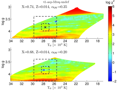
The set of frequencies for this exercise is composed of one mode of each degree444For clarity, hereafter, we use the notations and to refer to a mode of degree and radial order . =0 to 2 (see Table 3). The solutions obtained without classical constraints and on the sole seismic dataset as input are given in the 3rd column (No classical - m.f.) of Table 4. It predicts for , , and values of 15.6 , 10.18 , and 0.45, respectively. This fails at reproducing the true stellar parameter of the t1 model, and leads to a clear overestimation of overshooting. Figure 3 shows the map of the function in the – plane. For illustrating the discrepancy, the chemical composition and in the top panel are set to those of the solution: the global minimum clearly does not lie close to the input stellar parameters that were to be retrieved. The map also reveals regions with lower values under the form of ridges (blue patterns). They correspond to places of same . This is expected due to the presence of a radial mode in the input set and the direct dependence of radial modes to . However we see in the bottom panel of Fig. 3 that a local minimum is present at the correct – location when the chemical composition and of the t1 input model are adopted.

The solution obtained with the re-sampling method, presented in Sect. 2, is given in the 4th column (No classical - MC) of Table 4, still without including classical constraints. The inferred mass, with a value of 14.6 , is now close to that of the t1 input model (14 ) but the 1- error signals a low precision, 22%. The radius and the overshooting parameter are still significantly overestimated. We explain this trend in more detail hereafter.
Including classical constraints. When we require the solution to satisfy within 1- the and classical constraints, most of the stellar parameters of the input model are now correctly retrieved (see column 5 of Table 4), at the exceptions of and , which are underestimated by 0.10 and overestimated by 0.004, respectively. The determination of these two parameters actually presents a degeneracy. Indeed, the overshooting extends the main-sequence lifetime and also increases the luminosity of the evolutionary track. On the other hand, the chemical composition in the stellar envelope determines the opacity, hence the escaping radiation and luminosity: for a given mass, the lower the metallicity is, the higher the luminosity is. Stellar models with a given mass but with different combinations of overshooting and chemical composition can thus correspond to a same luminosity.

Figure 4 shows the map now in the – plane. It illustrates how the addition of the fundamental parameters as constraints discard the global minimum, which is outside the 1- box on and . However, despite the presence of a local minimum at the exact location of the target (bottom panel), the solution that is obtained remains inaccurate on some stellar parameters, as we have seen above. If we relax the precision on the classical parameters by considering a 3- error box, then the global minimum lies within that error box. Consequently, considering a too loose constraint (3- error box), or dealing with larger errors on classical parameters, which can be specially the case for , do not help improve the solution in comparison to that solely based on the seismic constraints.
With the inclusion of the classical parameters, the re-sampling method appears more robust. The inferred parameters then match those of the input model (see column 6 of Table 4). The errors at the 1- confidence level are down to 5% on the mass and 1.3% on the radius. Meanwhile the overshooting and metallicity are also correctly predicted, with an estimated precision of =0.004 and = 0.10. Again, the 3- classical constraints do not change the results of the MC simulations, providing the same results than without using the classical constraints.
The high-overshooting bias. To understand the tendency of the solution based on the only seismic dataset to favour high values of overshooting, we investigated in more detail the frequency spectra of the solutions emerging from the MC solutions. Before, it is useful to characterise some properties of the mixed modes. Firstly, the ratio of the vertical kinetic energy, , to the total kinetic energy, , reflects the dominant g- or p-character of an oscillation mode. The ratio is close to 0 for pure gravity modes, while it is equal to 1 for radial modes and typically greater than 0.9 for non-radial pressure modes. In the case of mixed modes, this ratio ranges in between these values.
Asymptotic developments allow to estimate the frequencies of pressure or gravity modes with help of simple relations based on the structural quantities of the stellar models (e.g. Shibahashi, 1979; Tassoul, 1980). In the case of low-degree pressure modes as in Cephei stars, these developments need in principle to include higher-order terms (Tassoul, 1990; Roxburgh & Vorontsov, 1994; Smeyers et al., 1996). Despite these levels of refinement, the asymptotic approach does not formally apply to low-radial order modes. However, it remains useful to estimate frequency values and relate them to the stellar structure properties, while it should not be used to compute the frequencies in a precise asteroseismic modelling of a Cephei star. An asymptotic expression of frequencies for acoustic modes reads as:
| (2) |
with the local sound speed, the radius defining the lower limit of the propagating cavity of the pressure mode, and a sum function wich includes as terms the number of nodes of the eigenfunction in that propagating cavity, , and other ones depending of the order of the approximation and the turning points of that cavity. When the mode is mixed with a dominant pressure character, the above expression includes a corrective term expressing the effect of the coupling between the g- and p-mode cavities (see details in e.g. Shibahashi, 1979). This term is of the order of , with 0 1. If the mode is well trapped inside the acoustic cavity, . Similar asymptotic expressions for the gravity modes can be derived, implying then the Brunt-Väisälä frequency, .
We can now inspect the frequency spectra from a sample of best-fit models from the MC simulation: the sample is built from solutions with values of 0.002 in the simulations that we have computed for this exercise. This gives a set of 20 models, which actually only 16 are different (solutions of different simulations can fall on a same model of the grid) . The parameters of these 16 models show a large spread in mass, from 11.2 to 18.1 , as well as in , with values from 0.20 to 0.50 but most of them presenting 0.45.


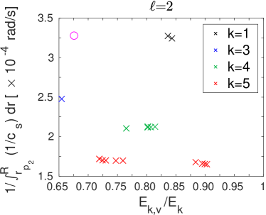
We compare in Fig. 5 the values of and the integral of Eq. (2) for the radial and non-radial modes in the 16 models that were best fitting the input frequencies. We can identify four groups. Black crosses correspond to the solutions in which the three fitting modes are: (), () and () modes. These radial orders and angular degrees are exactly the same as those of the t1-asp-3freq frequency set (magenta circles). The other three groups are composed of [; ; ] modes, with =2 (blue crosses), 3 (green crosses), and 4 (red crosses).
The models of the first group, as they reproduce exactly the order of the radial mode, have a similar than the t1 model. In the three other groups of models, each of the input frequencies is actually fitted by a mode of a higher overtone. The solutions with a radial mode presenting a higher present larger than the t1 model, since the proportionality of radial mode frequencies to includes a factor . We see in the top left panel that the solutions indeed gather around similar values of according to the radial order of their matching mode. The non-radial modes also gather according to their radial order (see top right and bottom panels). Two modes from two different stellar structures and with different radial orders will be characterised by values and in Eq. (2). The modes then will have a similar frequency value if the ratio of the integrals appearing in Eq. (2) is proportional to . Thus, the non-radial modes in Fig. 5 group according to because they have to reproduce a similar value of the ratio to present a frequency similar to, and hence fitting, that of the t1 model. As increases, so does , because it is . Consequently the inverses of the integrals of the modes with higher radial orders than the t1 case have to present lower values than the t1 inverse of the integral, as it is indeed observed in Fig. 5.
Overshooting now explains how models with different parameters can succeed in reproducing similar and inverse integrals of the sound speed. Most of the selected models present indeed higher overshooting values than the t1 model.
As we have seen, provided is higher than in the t1 model, higher overtone radial modes can match the frequency of the t1 fundamental radial mode. For models with large overshoot mixing, the range of values reached by their radius during the main sequence is increased. Since , these models will also evolve through a larger range of . This increases the probability that during their MS, a higher overtone in their frequency spectra matches that of the input radial mode, even if their fundamental radial mode would never present the same frequency than the t1 one.
Similarly, the increased variety of internal sound speed profiles and radii of a high-overshooting model will increase the range of values of their integrals for and modes. Therefore the probability also increases to reach a value of the integral, which the ratio with the t1 integral allows higher-overtones modes to reproduce the frequency of the lower-overtone t1 modes.
The use of the classical parameters has prevented this bias because they put an additional constraint on the radius and discarded models which did not reproduce . It is thus crucial to determine them independently with the highest accuracy and precision possible when a limited number of modes are considered for the asteroseismic modelling. Recently, the first interferometric measurement of the angular diameter of a Cephei star ( Can Maj) by Abeysekara et al. (2020) has reached a precision of %. In combination with Gaia parallaxes, the interferometric measurement of radii of Cephei stars would be a promising additional classical constraint on which to rely.
We also performed additional tests (not presented in detail here), first where a second mode instead of the one was considered in the input dataset. In that case, the results of the seismic modelling and the re-sampling method did not change for the mass, but gave accurate results for . The parameter overestimation was reduced (), and with the re-sampling method, it reduced to . The precision was not improved. The frequency spacing between mixed modes of same angular degree brings additional information on the structure, and reduces the probability to match frequency spectra by higher overtones of a model with a totally different structure. However, in another test where the three modes where all , the solution was significantly degraded. It appears clearly it came from a degeneracy on the determination on and in the absence on a constraint on through a radial mode.
In conclusion, the ranges of global stellar properties able to lead to a good fit of a small number of frequencies are quite large. Fitting these frequencies then do not allow to characterise reliably the input model, without help of additional constraints.
5.1.2 Four frequencies with known angular degree: The t1-asp-4freq test
The input set of frequencies is composed of one radial mode and three non-radial modes (2 , 1 ). The results are reported in Table 4: (0.014) and (0.20) are perfectly fitted, while the other stellar parameters are slightly underestimated with = 13.8 M⊙, = 7.45 , = 0.68, and = 0.274.
In comparison with the tests composed of three frequencies, we checked the map and found it contains fewer local minima. The global minimum lies now very close to the actual location of the t1 input model. With the re-sampling method, the inferred stellar parameters are then even closer to the t1 model (column 4 of Table 4). This method accounts for the theoretical uncertainties, which we have seen in Sect. 2.2 can be dominated by non-adiabatic effects. Here, as the target model and the model grid have the same physics, the non-adiabaticity of the input frequencies seems likely at the origin of the small inaccuracy in some of the retrieved stellar parameters.
Including classical constraints. With or without these constraints, the errors are very low in the three cases (columns 4,6, and 8 of Table 4), reaching a precision of 1% on and 0.005% on . As observed in the additional tests with three frequencies, the seismic modelling when it includes two mixed modes of same degree benefits from an information on the evanescent region. This region is a strong marker of the stellar structure as it is defined by the layers marking the transition between the core and radiative envelope.
5.1.3 Five frequencies with known angular degree: The t1-asp-5freq test
In this exercise, the number of seismic constraints is equal to the degrees of freedom of the problem, and would begin in principle to be optimal for adjusting the free parameters. The input frequency set is composed of the same frequencies than the t4-asp-op-4freq exercise, but includes one additional mode.
The model minimising appears to correspond to the same model that in the preceding exercise with only four frequencies, so that the inferred stellar parameters are identical. We observe similarly a significant decrease of the number of local minima and their value, which is illustrated in the top panel of Fig. 6. In comparison to the previous exercise, we observe an increased precision on the determination of the chemical composition and on , which reaches in this case the limit in precision of the grid. The stellar parameter distributions from the solutions of the MC simulations show that 80% of the models are characterised by = 0.20 and 70% of them present a mass of 13.8 or 13.9 M⊙.

An inaccuracy of 0.2 appears on the mass derived by the seismic modelling and is very likely related to the non-adiabatic computation of the input frequencies. It also reveals that the values we estimated for the errors could be underestimated, since the mass of the target is not predicted by our 1- interval of confidence: its upper limit predicts a mass of 13.9 , however only at 0.1 of the real value.

The present asteroseismic modelling has shown its ability to retrieve the global stellar parameters with high precision and accuracy. But we also find that it is able to determine the location of the central fully mixed region -the convective core and the overshooting region- both in terms of the radius and more importantly for stellar evolution, of mass with a high accuracy (see values in Table 5). In Fig. 7 the locations in term of the normalised mass, , of this region in the t1 target model and in the best-fit model match to less than 1%. Similarly, the gradient of chemical composition ( hereafter) above the boundary of the mixed region is also reproduced with an accuracy ¡1%. The shape and extent of this gradient are a marker of the extra-mixing processes. Succeeding in delivering a tight constraint on it is key to reveal the nature of these processes in massive stars.
| Exercise | ||||||||||||
|---|---|---|---|---|---|---|---|---|---|---|---|---|
| t1-asp-op-4freq | 0.153 | 0.194 | 0.154 | 0.193 | -0.007 | -0.005 | 0.315 | 0.319 | 0.448 | 0.448 | -0.01 | 0.00 |
| t1-asp-op-5freq | ||||||||||||
| t2-gn93 | 0.159 | 0.195 | 0.169 | 0.204 | -0.06 | -0.05 | 0.291 | 0.337 | 0.408 | 0.457 | -0.16 | -0.12 |
| t6-asp-diff | 0.152 | 0.233 | 0.158 | 0.191 | -0.04 | 0.18 | 0.237 | 0.222 | 0.471 | 0.337 | 0.06 | 0.28 |
Note: The variables indexed by and respectively represent those of the input target model and the output best-fit model from the exercise indicated in the first column.
As expected, the classical constraints do not improve further the modelling results and their errors. However, since the classical parameters are extracted from the t1 model, they do not suffer inaccuracy as could parameters derived from real conditions observations. The approach could thus be reversed in the study of observed Cephei stars by comparing whether parameters such as and seismically determined match their photometric or spectroscopic determinations. In particular, a clear discrepancy between the asteroseismic and spectroscopic was revealed by the modelling of several Cephei stars, as discussed in Aerts et al. (2011). These authors suggest the origin of the disagreement might be due to the pulsational broadening of lines not well accounted for in the spectroscopic analysis used for deriving the surface gravity.
5.2 Knowledge of the mode identification
We first analysed the impact of misidentifying a degree. In practice, although the methods555such as the moment method based on spectroscopic line variations (Balona, 1986; Aerts, 1996) or the analysis of photometric bandpass ratio Cugier et al. (1994). developed for identifying the modes in Cephei stars are generally able to constrain the angular degree of detected pulsations, in some cases the identification can be ambiguous. That was for example the case of Eri (see De Ridder et al., 2004, in particular their Figs. 5 and 6), whatever the method used. The same difficulty occurred for the photometric bandpass ratios analysis of the 12 Lac star (Handler et al., 2006). In a second time, we have focused on cases where no identification of the mode is possible, which is typically the case of stars observed in a single photometric bandpass.
5.2.1 Misidentifying a mode
We assume in the t1-1wrong exercise the same set of five frequencies as in the t1-asp-5freq case, but one of the modes is misidentified as an . The inferred parameters clearly fail at reproducing the t1 model: for instance, they give = 10.10 M⊙, = 10.45 R⊙, and = 0.004. As illustrated in the bottom panel of Fig. 6, the map degrades in comparison to the case where frequencies were correctly identified (top panel). The global minimum value signals the issue: it increases to = 85.162, about 200 to 400 times the corresponding values in the t1-asp-5freq and t1-asp-4freq exercises, respectively.
The best-fit model is evolved and close to the TAMS. Its frequency spectrum is denser than in a less-evolved stellar model. Fig. 8 depicts the frequency spectra of the and modes of this model, as well as the spectrum of the model t1. The grey dashed line indicates the input mode that is identified as an one. With the misidentification, the frequency spacing between the input modes is erroneously reduced. Since the input modes are associated to theoretical mode with the same degree, the solution is directed to models reproducing that erroneous feature, that is with denser frequency spectra, in a later stage of evolution.

Including the classical constraints. When imposing the solution to fall within the 1- error box on , the inferred parameters are improved; they predict = 14.2 M⊙, = 7.77 R⊙, and = 0.226, close to the t1 input ones. However, = 0 and a high of 0.018 appear in contradiction with the t1 parameters. The minimum, =554.05, again signals an issue with the result of the modelling.
5.2.2 Unknown identification of the modes
We determined the consequences of having no information on the angular degree through the t1--4unknown and t1--5unknown exercises. We took the same four and five frequencies than in the t1-asp-4freq and t1-asp-5freq tests, respectively, but without knowledge of their degrees. The results of the two exercises are given in Table 6.
| Exercise | Parameter | No constraint | 1- box constraint | 3- box constraint | |||
|---|---|---|---|---|---|---|---|
| m.f. | MC | m.f. | MC | m.f. | MC | ||
| t1-asp-4freq-undef | M (14) | 14.2 | 14.2 | 16.6 | 16.6 | 16.6 | 16.7 |
| R (7.48) | 9.99 | 10.02 | 9.43 | 9.43 | 9.43 | 9.64 | |
| X (0.70) | 0.72 | 0.72 | 0.70 | 0.70 | 0.70 | 0.72 | |
| Z (0.014) | 0.016 | 0.014 | 0.016 | 0.016 | 0.016 | 0.014 | |
| (0.20) | 0.35 | 0.35 | 0.15 | 0.15 | 0.15 | 0.25 | |
| (0.288) | 0.201 | 0.177 | 0.212 | 0.212 | 0.212 | 0.212 | |
| (27647) | 25197 | 25197 | 28084 | – | 28084 | – | |
| (3.8364) | 3.5909 | 3.5909 | 3.7087 | – | 3.7087 | – | |
| 0.0269 | – | 0.0427 | – | 0.0427 | – | ||
| t1-asp-5freq-undef | M (14) | 15 | 14.4 | 13.8 | 13.8 | 15 | 15 |
| R (7.48) | 10.16 | 10.04 | 7.45 | 7.45 | 10.16 | 10.10 | |
| X (0.70) | 0.74 | 0.72 | 0.68 | 0.68 | 0.74 | 0.72 | |
| Z (0.014) | 0.014 | 0.014 | 0.014 | 0.014 | 0.014 | 0.014 | |
| (0.20) | 0.35 | 0.35 | 0.20 | 0.20 | 0.35 | 0.35 | |
| (0.288) | 0.210 | 0.200 | 0.274 | 0.275 | 0.210 | 0.201 | |
| (27647) | 25699 | 25713 | 27888 | – | 27888 | – | |
| (3.8364) | 3.6001 | 3.5931 | 3.8330 | – | 3.6001 | – | |
| 0.2452 | – | 0.4175 | – | 0.2452 | – | ||
Same comments than in Table 4.
At first, with a set of four frequencies, the mass deduced is not too far away from the input one, but the radius and overshooting are overestimated to = 9.99 R⊙ and = 0.35, as reported in column 3 of Table 6.
In the top panel of Fig. 9, the map in the – plane for the output parameters clearly illustrates that the global minimum predicts an incorrect solution. A high number of local minima have appeared so that even the re-sampling method fails in this case to improve the results of the modelling. The local minima in the 1- or 3- error box on classical parameters provide as well wrong estimations of the stellar parameters (see columns 5 to 8 of Table 6). In the bottom panel of Fig. 9, the local minimum in the 1- error box is located at the very limit of the box, and also leads to wrong estimations of the mass (16.6 ) and radius (9.43 ).

Despite the poor results, the values of remain low, 0.02-0.03. The matching of the input modes by those of the grid is actually made easier. When a mode has its identified, it can only be matched to mode from the grid with a same . Yet, when is unknown, this mode can then be fitted by modes from the grid with =0 to 3, increasing the probabilities to match it with a mode of closer frequency, despite being of incorrect degree.
With the addition of one frequency in the t1--5unknow test, the global minimum and the results of the re-sampling method still lead to incorrect inferences when only based on the seismic dataset (see columns 3 and 4 of Table 6). In Fig. 10, the number of local minima is now reduced, yet revealing the impact of a supplementary frequency.
Including the classical constraints. With the help of the 1- constraints, the solution is significantly improved; the input stellar parameters are now determined with good accuracy. Furthermore, the results from the re-sampling method (column 6 of Table 6) present the same accuracy than in the t1-asp-5freq exercise. Yet, relaxing the constraint to the 3- constraints, the predicted stellar parameters do no longer fit those of the t1 model.
A reasonably large set of frequencies, although unidentified, can however lead to an accurate asteroseismic modelling, provided it is completed with tight constraints on the classical parameters. However, the stellar atmospheric parameters must be determined with a very good accuracy, as illustrated above when using the 3- error box on classical parameters.
5.3 Role of the input physics
We changed the physics of the model used as a target so that it differed from that of the grid. We examined the consequences on the quality of the global asteroseismic parameters, as well as on the constraints on the internal structure. We have seen in Sect.5.1.1 that there is a significant degeneracy for the determination of overshooting and metallicity. This degeneracy will be particularly accentuated if the detailed chemical composition of the star differs from that used in theoretical models. For instance, we recalled in Sect. 2.2 that between past determination of solar abundances like GN93 and the revision of AGS05, the metallicity decreased by 30%. Hence we tailored the t2-gn93 exercise to test the impact of the adopted composition. We used for the target t2 model the solar mixture of GN93, while it is the AGS05 mixture that is adopted in the grid. The other properties of the t2 models are given in Table 2. The set of input frequencies for the exercise are reported in Table 3 and is composed of six frequencies, with pairs of modes of degree ,, and .
| Exercise | Parameter | No constraint | 1- box constraint | 3- box constraint | |||
|---|---|---|---|---|---|---|---|
| m.f. | MC | m.f. | MC | m.f. | MC | ||
| t2-gn93 | M (11) | 11.4 | 11.4 | 11.5 | 11.4 | 11.4 | 11.4 |
| R (5.98) | 6.07 | 6.07 | 6.09 | 6.05 | 6.07 | 6.07 | |
| X (0.70) | 0.70 | 0.70 | 0.74 | 0.72 | 0.70 | 0.70 | |
| Z (0.016) | 0.012 | 0.012 | 0.014 | 0.014 | 0.012 | 0.012 | |
| (0.20) | 0.30 | 0.30 | 0.25 | 0.25 | 0.30 | 0.30 | |
| (0.351) | 0.354 | 0.354 | 0.385 | 0.373 | 0.354 | 0.354 | |
| (25293) | 26274 | 26274 | 25111 | – | 26274 | – | |
| (3.9258) | 3.9288 | 3.9288 | 3.9291 | – | 3.9288 | – | |
| 1.0338 | – | 2.5574 | – | 1.0338 | – | ||
| t6-asp-diff | M (10) | 10.2 | 10.2 | 10.2 | 10.2 | 10.2 | 10.2 |
| R (5.12) | 5.16 | 5.16 | 5.16 | 5.16 | 5.11 | 5.16 | |
| X (0.70) | 0.72 | 0.72 | 0.72 | 0.72 | 0.72 | 0.72 | |
| Z (0.014) | 0.016 | 0.016 | 0.016 | 0.016 | 0.016 | 0.016 | |
| (0†) | 0.05 | 0.05 | 0.05 | 0.05 | 0.05 | 0.05 | |
| (0.388) | 0.419 | 0.419 | 0.419 | 0.419 | 0.419 | 0.419 | |
| (24487) | 24015 | 24015 | 24015 | – | 24015 | – | |
| (4.0196) | 4.0212 | 4.0212 | 4.0212 | – | 4.0212 | – | |
| 2.5996 | – | 2.5996 | – | 2.5996 | – | ||
Same comments as in Table 4. Moreover, corresponds to input models with turbulent mixing: the extra mixing of the t6 models is equivalent to = 0.05.
The output parameters slightly overestimate the parameters of the t2 models with =11.4 and =6.07 . The best-fit model reproduces within 1% the one of the t2 model, confirming the influence of radial modes on the modelling. We see in the top panel of Fig. 11 that the lowest values of the merit function are indeed located in ridges, which actually correspond to places of equal . The parameters and are overestimated and underestimated, respectively (see column 3 of Table 7). This comes as expected from the degeneracy in and , accentuated by the difference in the chemical mixture. This effect was already observed in the modelling of HD129929, then from an ad hoc change in the mixture made by the authors (Thoul et al., 2004). Actually, in reason of the predominance of nuclear energy production by CNO cycle in B stars, for a given X and Z, a GN93 model will be more luminous than an AGS05 one. The reason is that C, N, and O are more abundant constituents of the metal mixture in the first case. Since we try to model a GN93 model with AGS05 models, the Z and likely adapt and do not correspond to those of the GN93 model.

Including the classical constraints. With predicted = 0.014 and = 0.25 (using 1- error box, see column 5 of Table 7), the discrepancy between the solution and the t2 model is reduced, but is now clearly overestimated, illustrating again the degeneracy on the overshooting and chemical composition determinations. The results of the re-sampling method are not very different (column 6 of Table 7), although the errors on the parameters are larger and so enclose the actual values of the t2 model. In Fig. 11, the global minimum and the lowest values of surrounding it, lie outside the 1- error box on the classical parameters (top panel). In the bottom panel, the local minimum found in the 1- error box is not well defined and its surrounding values are very similar: the solution is not well constrained, resulting in larger uncertainties on the derived parameters. The 3- constraints do not bring any information as the global minimum lies within it. This global minimum is clearly brighter and hotter than the target t2 model.

Overall, the inaccuracy induced by the difference in the chemical mixture remains limited to a few % on global parameters such as and . However, it is difficult to estimate the accuracy of parameters such as metallicity and overshooting given the degeneracy and compensatory role they play. Verifying how the limits of the convective core and are reproduced would better hint at the robustness of the asteroseismic modelling on this question. We present in Fig. 12 the internal profile of of the t2 and its seismic best-fit models, showing that the size in mass of the fully mixed regions and are not retrieved by the modelling (accuracy errors of 16 and 12%, respectively). Moreover, one mode (, ) of the input dataset is mixed with a dominant g-character, in principle an optimal information on these stellar layers. Yet, we see from Table 5 that the accuracy on these limits is much better in terms of , 5%. It highlights that the asteroseismic information is defined in terms of variables related to oscillations, so essentially sensitive to . While the acoustic structure of the star can be well reproduced, this is not necessarily the case of the mass distribution in the layers. Here it is clearly the difference in the chemical mixture that hinders the recovery of mass of the convective core and its overshooting region.
We did two other tests where the target models were computed with the GN93 mixture and with OPAL opacities (versus OP in the grid), but in one case, no overshooting was included. In both cases, the additional change in the physics did not alter precedent conclusion: we were still able to infer and with a good accuracy. But in the case with overshooting, we faced the same degeneracy on the chemical composition and overshooting determination. It resulted in an important discrepancy of 20% on the limit of the fully-mixed central region. Nevertheless, in the case without overshooting, the solution correctly retrieved the absence of overshooting (but failed at the chemical composition). The limits on the convective core were still of 5% in terms of , but remained of the same order when expressed in .
5.4 Nature of extra mixing
We have considered insofar models where the extra mixing was treated with a classical instantaneous prescription (see e.g. Maeder, 1975). Other processes can be responsible for extra mixing near the convective core, as for example turbulent mixing induced by rotation. Although this latter process has almost the same impact on the stellar evolutionary tracks as the overshooting (see e.g. Talon et al., 1997), the process acts like a diffusive process leading to smoother chemical composition gradients at the boundary of the convective core. The effect is in principle noticeable in comparison to the sharp profile generated in that same region by a very efficient mixing.
We explored this question in the t6-asp-diff exercise, in which turbulent mixing is implemented as a diffusive process parametrised by a turbulent diffusion coefficient, . We computed the t6 target model (see Table 2) with a value of = 70,000 cm.s-2, calibrated to correspond to a model computed with the Geneva code (Eggenberger et al., 2008) with an initial equatorial rotational velocity on the ZAMS () of 50 km/s. Doing so, the t6 model is equivalent (in terms of the extent of the central fully-mixed region) to a model without diffusive mixing but = 0.05.
The input frequency set is composed of two radial modes, three , and two modes. The modelling with these seismic constraints recovers with good accuracy , , and (see column 3 of Table 7), but and are overestimated.

The re-sampling method does not predict different results and it fails to determine consistent errors on the parameters (see column 4 of Table 7). The reason is that the global minimum is deeply marked in the map in Fig. 13, so that other solutions hardly emerge from the MC simulations. The global minimum lies within the 1- error box on –, and would do the same considering typical 1- observational error bars on . The classical constraints appear as no help in this case.
Of prime importance, we finally look at the limits of the convective core and in Fig. 14. The limit of the convective core is determined with a precision of 5% (see also Table 5) in , as it could be expected, since the t6 target model and the grid share the same chemical mixture (AGS05). However, the modelling fails at determining the location of , and so to be sensitive to the nature of the extra mixing. This is somehow expected as the grid did not include any diffusive mixing, confirming that getting constraints on the internal processes depends on the stellar models used. It suggests that a diffusive mixing should be as well considered in the grid for assessing its presence and efficiency in Cephei stars. This would add a degree of freedom, under the form of a diffusive coefficient taken as an additional parameter to adjust. Lovekin & Goupil (2010) tested the addition of a parameter in the fit, although applied to retrieve the rotation velocity of the star. Their results were encouraging as the convergence towards a reliable modelling of Cephei stars was not hindered by the additional parameter to fit.

We also did another test (not detailed here) considering a target model with diffusive mixing and the GN93 mixture, still with the grid only including instantaneous mixing. As expected, the inaccuracy increased, in particular on the determination of the convective core. Its inferred mass was then underestimated by 15%. The solution also exceeded by 15% the limit in on , confirming the insensitivity to the nature of extra mixing with an inappropriate model grid. Despite the internal structure was less-well characterised, the global stellar parameters were recovered with the same accuracy and precision than it the tests where the target stars included no diffusive mixing and the GN93 mixture in Sect. 5.3.
6 Conclusion
The asteroseismology of Cephei stars has already been applied in several occasions on well-characterised targets (see review by Aerts, 2015), leading to the derivation of the global parameters of these massive stars. These attempts also confirmed the potential for constraining internal processes such as rotation or mixing at the convective core boundary. With the latest results of the BRITE space mission, new seismic data extend the constraints for some well-known beta Cephei stars (Daszyńska-Daszkiewicz et al., 2017; Handler et al., 2017; Walczak et al., 2019). The first results of this mission have focused on the excitation of pulsation modes, confirming the call for a revision of stellar opacities, as previously stated from earlier studies on Cephei stars with fewer modes (Dziembowski & Pamyatnykh, 2008a; Montalban & Miglio, 2008; Salmon et al., 2012; Walczak et al., 2013; Daszyńska-Daszkiewicz et al., 2013; Cugier, 2014). The new data also give the opportunity to improve the snapshot of the internal structure that can be deduced with asteroseismology.
In this work, we explored in detail the role of the quality of the seismic data on precision and accuracy in the derivation of the stellar parameters and internal structure. We have developed a method that can be systematically applied to the modelling of Cephei stars. It is based on a re-sampling of the observed seismic frequencies, using Monte-Carlo simulations. It allows for instance to methodically estimate the errors on the derived parameters.
We applied this method in a series of hare and hound exercises, for which we simulated Cephei targets using theoretical stellar models. These tests aimed at defining the conditions required to obtain reliable and accurate seismic solutions. We also carefully characterised the dependence on the physics of stellar models used for the modelling. We explored the potential to determine the limits of the central mixed regions (convective core and overshoot region) as well as the nature of additional mixing processes at the convective core boundary. This would complement recent results obtained for SPBs (e.g. Pedersen et al., 2021), stars with a similar structure albeit less massive. The analysis of the exercises shows that:
-
•
Ideally the set of frequencies used for the modelling of a Cephei star should include at least four to five frequencies, with the knowledge of their angular degree (). Depending on the presence of mixed modes and the addition of fundamental parameters from non-seismic observables, accurate asteroseismic modelling with fewer modes is still possible, but is very dependent on the modes detected. The misidentification of one degree hindered to retrieve correctly the stellar parameters: but the value of the merit function was then significantly degraded, signalling the issue.
-
•
In the absence of identification of the modes, a set of four or five frequencies is not sufficient to determine the stellar parameters on the sole basis of the seismic dataset. Provided some fundamental parameters (effective temperature, surface gravity) are known from non-seismic constraints, we are able to retrieve the original stellar properties from a set of five frequencies.
-
•
If the nature of the extra mixing is the same between the star and the theoretical grid, the limit of the chemically homogeneous central regions (convective core plus overshoot region) is inferred with a good accuracy in terms of acoustic variables, like the radius. The extent of this region is correctly retrieved in terms of the mass provided the chemical mixture of the models is representative of the star. Therefore, the knowledge not only of the metallicity, but also of the individual chemical element abundances is required to identify the chemical mixture to be adopted. This encourages to systematically carry observations for determining the detailed abundances of Cephei stars.
-
•
When the nature of the extra mixing differs between the star and the theoretical grid, determining the size in mass of the convective core remains accurate when the chemical mixture of the grid reproduces that of the star. However, determining the limit of the chemical composition gradient and so the nature of the extra mixing appears unsuccessful. It hints at including in the analysis theoretical models with different treatments of the extra-mixing processes. Refined seismic diagnosis tools must be developed in that specific aim.
The re-sampling method based on Monte-Carlo method has demonstrated its capability to improve the results of the modelling when the solutions were initially poorly constrained. It also appears reliable to deliver realistic errors on the inferred parameters, as in most cases its error intervals were predicting correctly the real parameters of the target stellar models. It would be interesting to carry out further comparison with other statistical indicators in the future. For instance, we could perform a parallel analysis with the Mahalanobis distance, which use was proposed for asteroseismology of SPB pulsators by Aerts et al. (2018). This latter accounts directly for correlation between the parameters by including the covariances in its expression. The errors it predicts would be compared to those of our method. Yet, to compute correctly the covariance matrix, the required density and size of the grid of models have first to be estimated. As our method enables us to refine the region of the parameter space enclosing the solution, we could also use it as an exploratory method for providing initial guesses of a local method, such as the Levenberg-Marquardt algorithm (a two-step approach which was already followed for red-giants, e.g. Buldgen et al. 2019 or solar-like pulsators, e.g. Farnir et al. 2020).
Acknowledgements.
S.J.A.J.S., P.E., F.M. and G.M. have received funding from the European Research Council (ERC) under the European Union’s Horizon 2020 research and innovation programme (grant agreement No 833925, project STAREX). J.M. and A.M. acknowledge support from the European Research Council Consolidator Grant funding scheme (project ASTEROCHRONOMETRY, G.A. n. 772293, http://www.asterochronometry.eu). G.B. acknowledges funding from the SNF AMBIZIONE grant No. 185805 (Seismic inversions and modelling of transport processes in stars).References
- Abeysekara et al. (2020) Abeysekara, A. U., Benbow, W., Brill, A., et al. 2020, Nature Astronomy, 4, 1164
- Aerts (1996) Aerts, C. 1996, A&A, 314, 115
- Aerts (2013) Aerts, C. 2013, in EAS Publications Series, Vol. 64, EAS Publications Series, 323–330
- Aerts (2015) Aerts, C. 2015, in New Windows on Massive Stars, ed. G. Meynet, C. Georgy, J. Groh, & P. Stee, Vol. 307, 154–164
- Aerts et al. (2011) Aerts, C., Briquet, M., Degroote, P., Thoul, A., & van Hoolst, T. 2011, A&A, 534, A98
- Aerts et al. (2010) Aerts, C., Christensen-Dalsgaard, J., & Kurtz, D. 2010, Asteroseismology, Astronomy and Astrophysics Library (Springer)
- Aerts et al. (2004) Aerts, C., De Cat, P., Handler, G., et al. 2004, MNRAS, 347, 463
- Aerts et al. (2006) Aerts, C., Marchenko, S. V., Matthews, J. M., et al. 2006, ApJ, 642, 470
- Aerts et al. (2018) Aerts, C., Molenberghs, G., Michielsen, M., et al. 2018, ApJS, 237, 15
- Aerts et al. (2003) Aerts, C., Thoul, A., Daszyńska, J., et al. 2003, Science, 300, 1926
- Asplund et al. (2005) Asplund, M., Grevesse, N., & Sauval, A. J. 2005, in Astronomical Society of the Pacific Conference Series, Vol. 336, Cosmic Abundances as Records of Stellar Evolution and Nucleosynthesis, ed. T. G. Barnes III & F. N. Bash, 25
- Asplund et al. (2009) Asplund, M., Grevesse, N., Sauval, A. J., & Scott, P. 2009, ARA&A, 47, 481
- Badnell et al. (2005) Badnell, N. R., Bautista, M. A., Butler, K., et al. 2005, MNRAS, 360, 458
- Balona (1986) Balona, L. A. 1986, MNRAS, 219, 111
- Balona et al. (2011) Balona, L. A., Pigulski, A., Cat, P. D., et al. 2011, MNRAS, 413, 2403
- Bowman (2020) Bowman, D. M. 2020, Frontiers in Astronomy and Space Sciences, 7, 70
- Bowman & Michielsen (2021) Bowman, D. M. & Michielsen, M. 2021, A&A, in press
- Briquet et al. (2011) Briquet, M., Aerts, C., Baglin, A., et al. 2011, A&A, 527, A112
- Briquet et al. (2012a) Briquet, M., Neiner, C., Aerts, C., et al. 2012a, MNRAS, 427, 483
- Briquet et al. (2012b) Briquet, M., Neiner, C., Aerts, C., et al. 2012b, MNRAS, 427, 483
- Briquet et al. (2009) Briquet, M., Uytterhoeven, K., Morel, T., et al. 2009, A&A, 506, 269
- Buldgen et al. (2019) Buldgen, G., Farnir, M., Pezzotti, C., et al. 2019, A&A, 630, A126
- Burssens et al. (2020) Burssens, S., Simón-Díaz, S., Bowman, D. M., et al. 2020, A&A, 639, A81
- Caughlan & Fowler (1988) Caughlan, G. R. & Fowler, W. A. 1988, Atomic Data and Nuclear Data Tables, 40, 283
- Chiosi (2007) Chiosi, C. 2007, in IAU Symposium, Vol. 239, IAU Symposium, ed. F. Kupka, I. Roxburgh, & K. L. Chan, 235–246
- Chiosi & Maeder (1986) Chiosi, C. & Maeder, A. 1986, ARA&A, 24, 329
- Claret & Torres (2017) Claret, A. & Torres, G. 2017, ApJ, 849, 18
- Cox & Giuli (1968) Cox, J. P. & Giuli, R. T. 1968, Principles of stellar structure
- Cugier (2014) Cugier, H. 2014, A&A, 565, A76
- Cugier et al. (1994) Cugier, H., Dziembowski, W. A., & Pamyatnykh, A. A. 1994, A&A, 291, 143
- Daszyńska-Daszkiewicz et al. (2017) Daszyńska-Daszkiewicz, J., Pamyatnykh, A. A., Walczak, P., et al. 2017, MNRAS, 466, 2284
- Daszyńska-Daszkiewicz et al. (2013) Daszyńska-Daszkiewicz, J., Szewczuk, W., & Walczak, P. 2013, MNRAS, 431, 3396
- De Ridder et al. (2004) De Ridder, J., Telting, J. H., Balona, L. A., et al. 2004, MNRAS, 351, 324
- Degroote et al. (2010) Degroote, P., Aerts, C., Baglin, A., et al. 2010, Nature, 464, 259
- Degroote et al. (2012) Degroote, P., Aerts, C., Michel, E., et al. 2012, A&A, 542, A88
- Degroote et al. (2009) Degroote, P., Aerts, C., Ollivier, M., et al. 2009, A&A, 506, 471
- Deheuvels et al. (2016) Deheuvels, S., Brandão, I., Silva Aguirre, V., et al. 2016, A&A, 589, A93
- Dupret (2001) Dupret, M. A. 2001, A&A, 366, 166
- Dziembowski & Pamyatnykh (2008a) Dziembowski, W. A. & Pamyatnykh, A. A. 2008a, MNRAS, 385, 2061
- Dziembowski & Pamyatnykh (2008b) Dziembowski, W. A. & Pamyatnykh, A. A. 2008b, MNRAS, 385, 2061
- Eggenberger et al. (2008) Eggenberger, P., Meynet, G., Maeder, A., et al. 2008, Ap&SS, 316, 43
- Farnir et al. (2020) Farnir, M., Dupret, M. A., Salmon, S. J. A. J., Noels, A., & Buldgen, G. 2020, in Stars and their Variability Observed from Space, ed. C. Neiner, W. W. Weiss, D. Baade, R. E. Griffin, C. C. Lovekin, & A. F. J. Moffat, 281–286
- Formicola et al. (2004) Formicola et al. 2004, Physics Letters B, 591, 61
- Gallart et al. (2005) Gallart, C., Zoccali, M., & Aparicio, A. 2005, ARA&A, 43, 387
- Goupil (2011) Goupil, M. 2011, in Lecture Notes in Physics, Berlin Springer Verlag, Vol. 832, Lecture Notes in Physics, Berlin Springer Verlag, ed. J.-P. Rozelot & C. Neiner, 223
- Grevesse & Noels (1993) Grevesse, N. & Noels, A. 1993, in Origin and Evolution of the Elements, ed. N. Prantzos, E. Vangioni-Flam, & M. Casse, 15–25
- Handler et al. (2006) Handler, G., Jerzykiewicz, M., Rodríguez, E., et al. 2006, MNRAS, 365, 327
- Handler & Meingast (2011) Handler, G. & Meingast, S. 2011, A&A, 533, A70
- Handler et al. (2017) Handler, G., Rybicka, M., Popowicz, A., et al. 2017, MNRAS, 464, 2249
- Handler et al. (2004) Handler, G., Shobbrook, R. R., Jerzykiewicz, M., et al. 2004, MNRAS, 347, 454
- Labadie-Bartz et al. (2020) Labadie-Bartz, J., Handler, G., Pepper, J., et al. 2020, AJ, 160, 32
- Lovekin & Goupil (2010) Lovekin, C. C. & Goupil, M. J. 2010, A&A, 515, A58
- Maeder (1975) Maeder, A. 1975, A&A, 40, 303
- Maeder (1976) Maeder, A. 1976, A&A, 47, 389
- Mantegazza et al. (2012) Mantegazza, L., Poretti, E., Michel, E., et al. 2012, A&A, 542, A24
- Martinet et al. (2021) Martinet, S., Meynet, G., Ekström, S., et al. 2021, A&A, 648, A126
- Meynet et al. (2009) Meynet, G., Eggenberger, P., Mowlavi, N., & Maeder, A. 2009, in IAU Symposium, Vol. 258, IAU Symposium, ed. E. E. Mamajek, D. R. Soderblom, & R. F. G. Wyse, 177–188
- Michielsen et al. (2021) Michielsen, M., Aerts, C., & Bowman, D. M. 2021, A&A, 650, A175
- Michielsen et al. (2019) Michielsen, M., Pedersen, M. G., Augustson, K. C., Mathis, S., & Aerts, C. 2019, A&A, 628, A76
- Miglio et al. (2008a) Miglio, A., Montalbán, J., Eggenberger, P., & Noels, A. 2008a, Astronomische Nachrichten, 329, 529
- Miglio et al. (2009a) Miglio, A., Montalbán, J., Eggenberger, P., & Noels, A. 2009a, Communications in Asteroseismology, 158, 233
- Miglio et al. (2007) Miglio, A., Montalbán, J., & Maceroni, C. 2007, MNRAS, 377, 373
- Miglio et al. (2008b) Miglio, A., Montalbán, J., Noels, A., & Eggenberger, P. 2008b, MNRAS, 386, 1487
- Miglio et al. (2009b) Miglio, A., Montalbán, J., & Thoul, A. 2009b, Communications in Asteroseismology, 158, 280
- Montalban (1994) Montalban, J. 1994, A&A, 281, 421
- Montalban & Miglio (2008) Montalban, J. & Miglio, A. 2008, Communications in Asteroseismology, 157, 160
- Montalbán et al. (2008) Montalbán, J., Miglio, A., Eggenberger, P., & Noels, A. 2008, Astronomische Nachrichten, 329, 535
- Moravveji et al. (2016) Moravveji, E., Townsend, R. H. D., Aerts, C., & Mathis, S. 2016, ApJ, 823, 130
- Morel (2009) Morel, T. 2009, Communications in Asteroseismology, 158, 122
- Morel et al. (2006) Morel, T., Butler, K., Aerts, C., Neiner, C., & Briquet, M. 2006, A&A, 457, 651
- Moździerski et al. (2019) Moździerski, D., Pigulski, A., Kołaczkowski, Z., et al. 2019, A&A, 632, A95
- Niemczura et al. (2009) Niemczura, E., Morel, T., & Aerts, C. 2009, A&A, 506, 213
- Nieva & Przybilla (2012) Nieva, M.-F. & Przybilla, N. 2012, A&A, 539, A143
- Nieva & Simón-Díaz (2011) Nieva, M. F. & Simón-Díaz, S. 2011, A&A, 532, A2
- Pedersen et al. (2021) Pedersen, M. G., Aerts, C., Pápics, P. I., et al. 2021, Nature Astronomy, 5, 715
- Pedersen et al. (2018) Pedersen, M. G., Aerts, C., Pápics, P. I., & Rogers, T. M. 2018, A&A, 614, A128
- Pedersen et al. (2019) Pedersen, M. G., Chowdhury, S., Johnston, C., et al. 2019, ApJ, 872, L9
- Pinsonneault (1997) Pinsonneault, M. 1997, ARA&A, 35, 557
- Press (1981) Press, W. H. 1981, ApJ, 245, 286
- Przybilla et al. (2008) Przybilla, N., Nieva, M.-F., & Butler, K. 2008, ApJ, 688, L103
- Reese et al. (2016) Reese, D. R., Chaplin, W. J., Davies, G. R., et al. 2016, A&A, 592, A14
- Ribas et al. (2000) Ribas, I., Jordi, C., & Giménez, Á. 2000, MNRAS, 318, L55
- Rogers & Nayfonov (2002) Rogers, F. J. & Nayfonov, A. 2002, ApJ, 576, 1064
- Rogers & McElwaine (2017) Rogers, T. M. & McElwaine, J. N. 2017, ApJ, 848, L1
- Roxburgh & Vorontsov (1994) Roxburgh, I. W. & Vorontsov, S. V. 1994, MNRAS, 268, 143
- Salaris & Cassisi (2017) Salaris, M. & Cassisi, S. 2017, Royal Society Open Science, 4, 170192
- Salmon et al. (2012) Salmon, S., Montalbán, J., Morel, T., et al. 2012, MNRAS, 422, 3460
- Scott et al. (2021) Scott, L. J. A., Hirschi, R., Georgy, C., et al. 2021, MNRAS, 503, 4208
- Scuflaire (1974) Scuflaire, R. 1974, A&A, 36, 107
- Scuflaire et al. (2008a) Scuflaire, R., Montalbán, J., Théado, S., et al. 2008a, Ap&SS, 316, 149
- Scuflaire et al. (2008b) Scuflaire, R., Théado, S., Montalbán, J., et al. 2008b, Ap&SS, 316, 83
- Shibahashi (1979) Shibahashi, H. 1979, PASJ, 31, 87
- Smeyers et al. (1996) Smeyers, P., Vansimpsen, T., De Boeck, I., & Van Hoolst, T. 1996, A&A, 307, 105
- Stankov & Handler (2005) Stankov, A. & Handler, G. 2005, ApJS, 158, 193
- Szewczuk et al. (2021) Szewczuk, W., Walczak, P., & Daszyńska-Daszkiewicz, J. 2021, MNRAS, 503, 5894
- Talon & Charbonnel (2008) Talon, S. & Charbonnel, C. 2008, A&A, 482, 597
- Talon et al. (1997) Talon, S., Zahn, J.-P., Maeder, A., & Meynet, G. 1997, A&A, 322, 209
- Tassoul (1980) Tassoul, M. 1980, ApJS, 43, 469
- Tassoul (1990) Tassoul, M. 1990, ApJ, 358, 313
- Thoul et al. (2003) Thoul, A., Ausseloos, M., Barban, C., et al. 2003, Communications in Asteroseismology, 143, 25
- Thoul et al. (2004) Thoul, A., Scuflaire, R., Ausseloos, M., Aerts, C., & Noels, A. 2004, Communications in Asteroseismology, 144, 35
- Van Grootel et al. (2008) Van Grootel, V., Charpinet, S., Fontaine, G., et al. 2008, A&A, 488, 685
- Walczak et al. (2013) Walczak, P., Daszyńska-Daszkiewicz, J., Pamyatnykh, A. A., & Zdravkov, T. 2013, MNRAS, 432, 822
- Walczak et al. (2019) Walczak, P., Daszyńska-Daszkiewicz, J., Pigulski, A., et al. 2019, MNRAS, 485, 3544