An enhanced Kogbetliantz method for the singular value
decomposition (SVD) of general matrices of order two is proposed.
The method consists of three phases: an almost exact prescaling,
that can be beneficial to the LAPACK’s xLASV2 routine for
the SVD of upper triangular matrices as well, a highly
relatively accurate triangularization in the absence of underflows,
and an alternative procedure for computing the SVD of triangular
matrices, that employs the correctly rounded function. A
heuristic for improving numerical orthogonality of the left singular
vectors is also presented and tested on a wide spectrum of random
input matrices. On upper triangular matrices under test, the
proposed method, unlike xLASV2, finds both singular values
with high relative accuracy as long as the input elements are within
a safe range that is almost as wide as the entire normal range. On
general matrices of order two, the method’s safe range for which the
smaller singular values remain accurate is of about half the width
of the normal range.
keywords:
singular value decomposition, the Kogbetliantz method, matrices of order two, roundoff analysis
pacs:
[
MSC Classification]65F15, 15A18, 65Y99
1 Introduction
The singular value decomposition (SVD) of a square matrix of order two
is a widely used numerical tool. In LAPACK [1]
alone, its xLASV2 routine for the SVD of real upper
triangular matrices is a building block for the QZ
algorithm [2] for the generalized eigenvalue
problem , with and real and square, and for the
SVD of real bidiagonal matrices by the implicit QR
algorithm [3]. Also, the oldest method for the SVD
of square matrices that is still in use was developed by
Kogbetliantz [4], based on the SVD of order two,
and as such is the primary motivation for this research.
This work explores how to compute the SVD of a general matrix
of order two indirectly, by a careful scaling, a highly relatively
accurate triangularization if the matrix indeed contains no zeros, and
an alternative triangular SVD method, since the straightforward
formulas for general matrices are challenging to be evaluated stably.
Let be a square real matrix of order . The SVD of is a
decomposition , where and are
orthogonal111If is complex, and are unitary and
, but this case is only briefly dealt with here.
matrices of order of the left and the right singular vectors of
, respectively, and is
a diagonal matrix of its singular values, such that
for all and where
.
In the step of the Kogbetliantz SVD method, a pivot submatrix of
order two (or several of them, not sharing indices with each other,
if the method is parallel) is found according to the chosen pivot
strategy in the iteration matrix , its SVD is computed, and
, , and are updated by the transformation matrices
and/or , leaving zeros in the
off-diagonal positions and of , as in
(1)
The left and the right singular vectors of the pivot matrix are
embedded into identities to get and ,
respectively, with the index mapping from matrices of order two to
and being ,
, ,
, where are the pivot
indices. The process is repeated until convergence, i.e., until for
some the off-diagonal norm of falls below a certain
threshold.
If has rows and columns, , it should be
preprocessed [5] to a square matrix by a
factorization of the URV [6] type (e.g., the QR
factorization with column pivoting [7]).
Then, , where is triangular of order
and is orthogonal of order . If , then the SVD of
can be computed instead.
In all iterations it would be beneficial to have the pivot matrix
triangular, since its SVD can be computed with high
relative accuracy under mild assumptions [8]. This
is however not possible with time consuming but simple,
quadratically convergent [9, Remark 6] pivot
strategy that chooses the pivot with the largest off-diagonal norm
, but is possible,
if is triangular, with certain sequential cyclic (i.e.,
periodic)
strategies [5, 10] like the
row-cyclic and column-cyclic, and even with some parallel ones, after
further preprocessing into a suitable “butterfly”
form [11].
Although the row-cyclic and column-cyclic strategies ensure
global [10] and asymptotically
quadratic [9, 12] convergence of the
method, as well as its high relative accuracy [13],
the method’s sequential variants remain slow on modern hardware, while
preprocessing to (in the butterfly form or not) can only be
partially parallelized.
This work is a part of a broader
effort [14, 15] to investigate if a
fast and accurate (in practice if not in theory) variant of the
Kogbetliantz method could be developed, that would be entirely
parallel and would function on general square matrices without
expensive preprocessing, with full pivots ,
, that are independently
diagonalized, and with ensuing concurrent updates of
, of , and from each of the sides
of in a parallel step. This way the employed parallel pivot
strategy does not have to be cyclic. A promising candidate is the
dynamic
ordering [16, 17, 15].
The proposed Kogbetliantz SVD of order two supports a wider exponent
range of the elements of a triangular input matrix for which both
singular values are computed with high relative accuracy than
xLAEV2, although the latter is slightly more accurate when
comparison is possible. Matrices of the singular vectors obtained by
the proposed method are noticeably more numerically orthogonal. With
respect to [14, 15] and a general
matrix of order two, the following enhancements have been
implemented:
1.
The structure of is exploited to the utmost extent, so the
triangularization and a stronger scaling is employed only when
has no zeros, thus preserving accuracy.
2.
The triangularization of by a special URV factorization is
tweaked so that high relative accuracy of each computed element is
provable when no underflow occurs.
3.
The SVD procedure for triangular matrices utilizes the latest
advances in computing the correctly rounded functions, so the
pertinent formulas from [14, 15] are
altered.
4.
The left singular vectors are computed by a heuristic when the
triangularization is involved, by composing the two plane
rotations—one from the URV factorization, and the other from the
triangular SVD—into one without the matrix multiplication.
High relative accuracy of the singular values of is observed, but
not proved, when the range of the elements of is narrower than
about half of the entire normal range.
This paper is organized as follows. In Section 2 the
floating-point environment and the required operations are described,
and some auxiliary results regarding them are proved.
Section 3 presents the proposed SVD method. In
Section 4 the numerical testing results are shown.
Section 5 concludes the paper with the comments on future
work.
2 Floating-point considerations
Let be a real, infinite, or undefined (Not-a-Number) value:
. Its floating-point
representation is denoted by and is obtained by rounding
to a value of the chosen standard floating-point datatype using
the rounding mode in effect, that is here assumed to be to
nearest (ties to even). If the result is normal,
, where
and is the number of bits in the significand of a floating-point
value. In the LAPACK’s terms,
, where
or D. Thus,
or , and
or for single
(S) or double (D) precision, respectively. The
gradual underflow mode, allowing subnormal inputs and outputs, has to
be enabled (e.g., on Intel-compatible architectures the
Denormals-Are-Zero and Flush-To-Zero modes have to be turned off).
Trapping on floating-point exceptions has to be disabled (what is the
default non-stop handling from [18, Sect. 7.1]).
Possible discretization errors in input data are ignored.
Input matrices in floating-point are thus considered exact, and are,
for simplicity, required to have finite elements.
The Fused Multiply-and-Add (FMA) function,
, is required. Conceptually, the exact
value of is correctly rounded. Also, the hypotenuse
function, , is assumed to be
correctly rounded (unless stated otherwise), as recommended by the
standard [18, Sect. 9.2], but
unlike222https://members.loria.fr/PZimmermann/papers/accuracy.pdf
many current implementations of the routines hypotf and
hypot. Such a function (see also [19]) never
overflows when the rounded result should be finite, it is zero if and
only if , and is symmetric and monotone. The CORE-MATH
library [20] provides an open-source
implementation333https://core-math.gitlabpages.inria.fr
of some of the optional correctly rounded single and double precision
mathematical C functions (e.g., cr_hypotf and
cr_hypot).
Radix two is assumed for floating-point values. Scaling of a value
by where is exact if the result is normal.
Only non-normal results can lose precision. Let, for ,
and , and for a finite non-zero let the exponent be
and the “mantissa” , such
that . Also, let for , while
. Note that is normal even for subnormal . Keep in
mind that the frexp routine represents a finite non-zero
with and .
Let be the smallest and the largest positive finite normal
value. Then, in the notation just introduced,
or , and or , for
single or double precision. Lemma 2.1 can now be stated using
this notation.
Lemma 2.1.
Assume that , with rounding to nearest. Then,
(2)
Proof.
By the assumption, , since
, with ones. The bit in the
last place thus represents a value of at least four. Adding one to
would require rounding of the exact value
to bits of
significand. The number of zeros is . Rounding to
nearest in such a case is equivalent to truncating the trailing
bits, starting from the leftmost zero, giving the
result . This proves the
first equality in (2).
For the second equality in (2), note that
since . By taking
the square roots, it follows that ,
and therefore
since and are monotone operations in all arguments.
∎
The claims of Lemma 2.1 and its following corollaries were used
and their proofs partially sketched in [21], e.g. They
are expanded and clarified here for completeness.
An underlined expression denotes a computed floating-point
approximation of the exact value of that expression. Given
, for , and
are
(3)
if and are finite, or
and otherwise.
Corollary 2.2.
Let be given, such that is finite.
Then, under the assumptions of Lemma 2.1, for
from (3) holds
.
Proof.
For , due to Lemma 2.1,
, and so the denominator
in (3) is . Note that the
numerator is always at most as large in magnitude as the
denominator. Thus, , what had to
be proven.
∎
Corollary 2.3.
Let be given, for . Then,
can be approximated as
. If
, then
. When the assumptions of
Lemma 2.1 hold and is finite, so is
.
Proof.
The approximation relation follows from the definition of
and from , while its finiteness for a
finite follows from Lemma 2.1, since
implies .
∎
For any , let and
. Even such that
or , where is the smallest
positive non-zero floating-point value, can be represented with a
finite and a normalized , though is not
finite or non-zero, respectively. The closest double precision
approximation of is
, with a possible
underflow or overflow, and similarly for single precision (using
scalbnf). A similar definition could be made with and
instead.
An overflow-avoiding addition and an underflow-avoiding subtraction of
positive finite values and , resulting in such
exponent-“mantissa” pairs, can be defined as
Assume (else, swap and , and change the sign of ).
Then, and
. The
rightmost bit multiplies the value
.
If then is normal and, due to rounding to
nearest, . Therefore, assume that . If
, then as well, since .
Thus, , so assume that , i.e.,
.
It now suffices to upscale and to and
, for some , to ensure
. Any
that will not overflow will do,
so the smallest one is chosen. Note that
. Since
, by the Lemma’s assumption it holds
.
∎
Several arithmetic operations on -pairs can be defined (see
also [22]), such as
(6)
which are unary operations. The binary multiplication and division
are defined as
(7)
and the relation , that compares the represented values in the
sense, is given as
(8)
Let, for any of order , where INT_MIN is the smallest
representable integer,
(9)
A prescaling of as , that avoids overflows,
and underflows if possible, in the course of computing the SVD of
(and thus of
), is defined by such
that
(10)
where for . For , is chosen
such that certain intermediate results while computing the SVD of
cannot overflow, as explained
in [14, 15] and Section 3, but
the final singular values are represented in the form, and are
immune from overflow and underflow as long as they are not converted
to simple floating-point values. If , the result of such a
prescaling is exact. Otherwise, some elements of
might be computed inexactly due to underflow. If for the elements of
holds
(11)
then , and or , i.e., the
elements of are zero or normal.
3 The SVD of general matrices of order two
This section presents a Kogbetliantz-like procedure for computing the
singular values of when , and the matrices of the left ()
and the right () singular vectors.
In general, is a product of permutations (denoted by with
subscripts and including ), sign matrices (denoted by with
subscripts) with each diagonal element being either or while
the rest are zeros, and plane rotations by the angles and
. If is not generated, the notation changes
from to . Likewise, is a product of
permutations, a sign matrix, and a plane rotation by the angle ,
where
(12)
Depending on its pattern of zeros, a matrix of order two falls into
one of the 16 types shown in (13), where
and . Some types are permutationally
equivalent to others, what is denoted by
, and means that a
-matrix can be pre-multiplied and/or post-multiplied
by permutations to be transformed into a -matrix, and
vice versa, keeping the number of zeros intact. Each
has its associated scale type .
(13)
For , there is one equivalence class of matrix types,
represented by . For , there are
three classes, represented by , , and
, while for there is one class,
. The SVD computation for the first three classes is
straightforward, while for the fourth and the fifth class is more
involved. A matrix of any type, except , can be
permuted into an upper triangular one. If a matrix so obtained is
well scaled, its SVD can alternatively be computed by xLASV2.
However, xLASV2 does not accept general matrices (i.e.,
), unlike the proposed method, which is a
modification of [15] when , and consists of
the following three phases:
1.
For determine , , and to
obtain . Handle the simple cases of
separately.
2.
If or , factorize
as , such that and
are orthogonal, and is upper triangular, with
and all finite,
.
3.
From the SVD of assemble the SVD of
. Optionally backscale by
.
The phases 1, 2, and 3 are described in Sections 3.1,
3.2, and 3.3, respectively.
3.1 Prescaling of the matrix and the simple cases ()
Matrices with do not have to be scaled, but only
permuted into the , , or
(where the first diagonal element is not smaller by
magnitude than the second one) form, according to their number of
non-zeros, with at most one permutation from the left and at most one
from the right hand side. Then, the rows of are
multiplied by the signs of their diagonal elements, to obtain
and , while and
. The error-free SVD computation is thus completed.
Note that the signs might have been taken out of the columns instead
of the rows, and the sign matrix would have then be incorporated
into instead. The structure of the left and the right singular
vector matrices is therefore not uniquely determined.
Be aware that determined before the prescaling (to
compute and ) may differ from that
would be found afterwards. If, e.g., and
contains, among others, and as elements, the
element(s) will vanish after the prescaling since
(from (10), due to ), so
and the zero pattern of
has to be re-examined.
A or matrix is scaled by
. The columns (resp., rows) of a (resp.,
) matrix are swapped, to bring it to the
(resp., ) form. Then, the
non-zero elements are made positive by multiplying the rows (resp.,
columns) by their signs. Next, the rows (resp., columns) are swapped
if required to make the upper left element largest by magnitude. The
sign-extracting and magnitude-ordering operations may be swapped or
combined. The resulting matrix undergoes the QR (resp., RQ)
factorization, by a single Givens rotation (resp.,
), determined by (consequently, by
and ) as in (12), with
substituted for (resp., ), where
(14)
By construction, and
. The upper left element is not
transformed, but explicitly set to hold the Frobenius norm of the
whole non-zero column (resp., row), as
(resp.,
),
while the other non-zero element is zeroed out. Thus, to avoid
overflow of it is sufficient to ensure that
, what achieves.
The SVD is given by and for
, and by and
for . The scaled
singular values are and in both
cases, and cannot overflow
( can).
If no inexact underflow occurs while scaling to , then
, where
. With the same assumption,
implies
, where
. The resulting Givens rotation
can be represented and applied as one of
(15)
what avoids computing and
explicitly. Lemma 3.1 bounds the
error in .
By adding unity to both sides of the equation for
and taking the maximal value of the first
factor on its right hand side, while accounting for the bounds of
, it holds
Since
,
where , factorizing the
last square root into a product of square roots gives
The proof is concluded by denoting the error factor on the right
hand side by .
∎
This proof and the following one use several techniques
from [21, Theorem 1]. Due to the structure of a matrix
that or is applied to, containing in
each row and column one zero and one , it follows that or
have in each row and column and
, computed implicitly, for which
Lemma 3.2 gives error bounds.
If, in (14), , then
since
, and the
relative error in is below for
any standard floating-point datatype. Thus, even though
can be relatively inaccurate,
(16) holds for all .
Also, is always relatively
accurate, but might not be if
, when
.
3.2 A (pivoted) factorization of order two ()
If, after the prescaling, or
, is transformed into an upper
triangular matrix with all elements non-negative, i.e., a special
URV factorization of is computed.
Section 3.2.1 deals with the , and
Section 3.2.2 with the case.
3.2.1 An error-free transformation from to form
A triangular or anti-triangular matrix is first permuted into an upper
triangular one, . Its first row is then multiplied by the sign
of . This might change the sign of . The second
column is multiplied by its new sign, what might change the
sign of . Its new sign then multiplies the second row, what
completes the construction of .
The transformations and , such that
, can be expressed as
and
, and are exact, as well as
if is.
3.2.2 A fully pivoted URV when
In all previous cases, a sequence of error-free transformations would
bring into an upper triangular , of which xLASV2
can compute the SVD. However, a matrix without zeros either has to
be preprocessed into such a form, in the spirit
of [14, 15], or its SVD has to computed
by more complicated and numerically less stable formulas, that follow
from the annihilation requirement for the off-diagonal matrix elements
as
(19)
A sketched derivation of (19) can be found in Section 1 of
the supplementary material.
Opting for the first approach, compute the Frobenius norms of the
columns of , as and . Due to the prescaling,
and
cannot overflow. If , swap the columns and their norms
(so that would be the norm of the new first column of
, and the norm of the second one). Multiply
each row by the sign of its new first element to get . Swap the
rows if to get the fully pivoted , while the
norms remain unchanged. Note that .
Now the QR factorization of is computed as
. Then, , and
(20)
All properties of the functions of from Section 3.1
also hold for the functions of . The prescaling of
causes the elements of to be at most in
magnitude.
If , then , and if
, then . In either case
is processed further as in Section 3.1,
while accounting for the already applied transformations. Else, the
second column of is multiplied by the sign of to
obtain . The second row of is multiplied by the sign of
to finalize , in which the upper triangle is positive.
It is evident how to construct and
such that , since
(21)
However, is not explicitly formed, as
explained in Section 3.3. Now for
.
Lemma 3.3 bounds the relative errors in (some of) the elements
of , when possible.
Lemma 3.3.
Assume that no inexact underflow occurs at any stage of the above
computation, leading from to . Then,
, where
(22)
If in
holds , then
and
, where
(23)
Else, if and are of
the same sign, then , and
if they are of the opposite signs, then
, where, with
and ,
(24)
Proof.
Eq. (22) follows from the correct rounding of
in the computation of .
To prove (23) and (24), solve
for with . After expanding and
rearranging the terms, it follows that
(25)
If and are of the same sign and the addition operation is
chosen, the first factor on the first right hand side
in (25) is above zero and below unity, so
and
(26)
The same holds if and are of the opposite signs and the
subtraction is taken instead. Specifically, from (20),
the bound (26) holds for and
of the same sign, with , and for
and of the
opposite signs, with .
With and
, from the definition of
it follows that
(27)
Due to (16) and (27), with
instead of and with where
, it holds
(28)
where for and for . Now (23)
follows from bounding
below
and above using (16). Since
in (28),
(24) is a consequence of (23).
∎
Lemma 3.3 thus shows that high relative accuracy of all elements
of is achieved if no underflow has occurred at any
stage, and has been computed exactly. If
is inexact, high relative accuracy is
guaranteed for and exactly one of
and . If it is also desired
for the remaining element, transformed by an essential subtraction and
thus amenable to cancellation, one possibility is to compute it by an
expression equivalent to (20), but with
expanded to its definition , as in
(29)
after prescaling the numerator and denominator in (29) by the
largest power-of-two that avoids overflow of both of them. A
floating-point primitive of the form with a
single rounding [23] can give the correctly rounded
numerator but it has to be emulated in software on most platforms at
present [24]. For high relative accuracy of
or the absence of
inexact underflows is required, except in the prescaling.
Alternatively, the numerators in (29) can be calculated by the
Kahan’s algorithm for determinants of order
two [25], but an overflow-avoiding prescaling is
still necessary. It is thus easier to resort to
computing (29) in a wider and more precise datatype as
(30)
First, in (30) it is assumed that no underflow has occurred so
far, so . Second, a product of two
floating-point values requires bits of the significand to be
represented exactly if the factors’ significands are encoded with
bits each. Thus, for single precision, bits are needed, what is
less than bits available in double precision. Similarly, for
double precision, bits are needed, what is less than bits
of a quadruple precision significand. Therefore, every product
in (30) is exact if computed using a more precise standard
datatype T. The characteristic values of T are the
underflow and overflow thresholds and
, and
. Third,
let round an infinitely precise result of to the nearest
value in T. Since all addends in (30) are exact and
way above the underflow threshold by
magnitude, the rounded result of the addition or the subtraction is
relatively accurate, with the error factor ,
. This holds
even if the result is zero, but since the transformed matrix would
then be processed according to its new structure, assume that the
result is normal in T. The ensuing division cannot overflow
nor underflow in T. Now the quotient rounded by is
rounded again, by , back to the working datatype. This operation
can underflow, as well as the following division by
. If they do not, the resulting
transformed element is relatively accurate. This outlines the
proof of Theorem 3.4.
Theorem 3.4.
Assume that no underflow occurs at any stage of the computation
leading from to . Then,
, where for
holds (22). If is exact, then
and
, where and
are as in (23). Else, if
and are of the same
sign, then and
. If they are of the
opposite signs, then and
, where and
are as in (24), while and
come from evaluating their corresponding matrix
elements as in (30) and are bounded as
(31)
Proof.
It remains to prove (31), since the other relations follow
from Lemma 3.3.
Every element of is not above and not below in
magnitude. Therefore, a difference (in essence) of their exact
products cannot exceed in
magnitude in a standard T. At least one element is above
in magnitude due to the prescaling, so the said difference,
if not exactly zero, is above
in magnitude.
Thus, the quotient of this difference and is above
and, due to the prescaling and pivoting, not above
in magnitude. For (30)
it therefore holds
(32)
The quotient , converted
to the working precision with
, is possibly not
correctly rounded from the value of
due to its double rounding.
Using the assumption that no underflow in the working precision
occurs, it follows that
(33)
with
.
For the final division by , due
to (16), holds
(34)
By fixing the sign in the subscript in (32),
(33), and (34), let
and
. Now bound
and below by and above by
, by combining the appropriate lower and upper bounds
for , from
Lemma 3.1, and , where
what proves (31), by minimizing the numerator and maximizing
the denominator to minimize the expression for and
, and vice versa, as in the proof of Lemma 3.3.
∎
Therefore, it is possible to compute with high
relative accuracy in the absence of underflows, in the working
precision only, but it is easier to employ two multiplications, one
addition or subtraction, and one division in a wider, more precise
datatype. Table 1 shows by how many s the lower
and the upper bounds for , , and
from (23), (24), and (31), respectively,
differ from unity. The quantities in the table’s header were computed
symbolically as algebraic expressions by substituting
and with their defining powers of
two, then approximated numerically with
decimal digits, and rounded upwards to nine digits after the decimal
point, by a Wolfram Language script444The relerr.wls
file in the code supplement, executed by the Wolfram Engine 14.0.0 for
macOS (Intel)..
Table 1: Lower and upper bounds for , , and in single and double precision.
\topruleprecision
\midrulesingle
3.499999665
3.500000336
4.499999457
4.500000544
3.499999669
3.500000340
double
3.500000000
3.500000001
4.500000000
4.500000001
3.500000000
3.500000001
\botrule
3.3 The SVD of and
For now holds . If
, the diagonal elements of
have to be swapped, similarly to xLASV2.
This is done by symmetrically permuting with
.
Multiplying
by from the left and from the right gives
where ,
, and
. Therefore, having applied the
permutation ,
(35)
where , , and
come from the SVD of in
Section 3.3.1. If
then ,
, , (35) is
not used, and let , ,
and .
Assume that no inexact underflow occurs in the computation of
. If the initial matrix was triangular, let
. Else, let ,
, and stand for the error factors of the
elements of that correspond to those from
Theorem 3.4, i.e.,
(36)
It remains to compute the SVD of by an
alternative to xLASV2, what is described in
Section 3.3.1, and assemble the SVD of , what is
explained in Section 3.3.2.
3.3.1 The SVD of
The key observation in this part is that the
traditional [5, Eq. (4.12)] formula for
involving the squares of the elements of
can be simplified to an expression that does not
require any explicit squaring if the hypotenuse calculation is
considered a basic arithmetic operation. The two following
expressions for are equivalent,
(37)
With
, let
and
be the sum
and the difference555With the prescaling as employed, can be replaced
by subtraction and . of
and as in (4)
and (5), respectively, for
. From (36) and
since for , it
holds
.
Thus (37) can be re-written using (6)
and (7), with
and
,
as
(38)
where the computation’s precision is unchanged, but the exponent range
is widened.
In (19), the denominator of the expression for
,
,
can also be computed using , without explicitly squaring
any matrix element, as
Only if can happen that
.
In the first denominator in (37),
and then have a negligible
effect on , so the expression for
can be simplified, as in xLASV2,
to the same formula which would the case
imply,
(39)
Let
.
If ,
(37) can be simplified by explicit squaring to
(40)
Both (39) and (40) admit a simple roundoff
analysis. However, (38) does not, due to a subtraction of
potentially inexact values of a similar magnitude when computing
. Section 4 shows, with a high probability by an
exhaustive testing, that (38) does not cause excessive
relative errors in the singular values for ,
and neither for if the range of the exponents of
the elements of input matrices is limited in width to about
. If is not correctly rounded, the
procedure from [14, 15] for computing
without squaring the input values can be
adopted instead of (38), as shown in Algorithm 1,
but still without theoretical relative error bounds.
Algorithm 1 Computation of the functions of from .
All cases of Algorithm 1 lead to
. From
follows , as well as
and , when
explicitly required, what completely determines
.
To determine , is
obtained from (see [5, Eq. (4.10)])
as
(41)
Let
.
If is finite (e.g., when ,
due to the pivoting [14, Theorem 1]), so is
. Then, let
.
By fixing the evaluation order for reproducibility, the singular
values and of
are
computed [8, 15] as
(42)
If overflows due to a small
(the prescaling ensures that
is always finite), let
. In this case,
similarly to the one in xLASV2 for
,
it holds , so
. To confine subnormal values to
outputs only, let
(43)
By substituting
from (43) for in (42),
simplifying the results, and fixing the evaluation order, the singular
values of in this case are obtained as
(44)
From (41), implies
,
so . Therefore,
may be eliminated from (44),
similarly as in xLASV2.
The SVD of has thus been computed (without
explicitly forming and
) as
(45)
If , then
,
, and
,
else and
, as presented in Algorithm 2.
If then
should be formed as in (35), and
as well if . Else, if
, then
, and (only
implicitly for )
.
Algorithm 2 Computation of the functions of and the singular values of .
The approximate backscaled singular values of are
. They should
remain in the exponent-“mantissa” form if possible, to avoid
overflows and underflows.
Recall that, for ,
and the QR rotation
have not been explicitly formed. The
reason is that
,
where is constructed from
as in (21), requires a
matrix-matrix multiplication that can and sporadically will degrade
the numerical orthogonality of . On its own,
such a problem is expected and can be tolerated, but if the left
singular vectors of a pivot submatrix are applied to a pair of pivot
rows of a large iteration matrix, many times throughout the
Kogbetliantz process (1), it is imperative to make the vectors as
orthogonal as possible, and thus try not to destroy the singular
values of the iteration matrix. In the following,
is generated from a single
, where is a function of the
already computed and .
If , let
, where
comes from Section 3.2.1. Else, due
to (35), if in (21), the product
can be written in the terms of as
(46)
If
,
can be written in the terms of as
(47)
what is obtained by multiplying the matrices
and simplifying the result using the trigonometric identities for the
(co)sine of the difference of the angles and
. The middle matrix factor represents a possible sign
change of as in Section 3.2.2. The matrices
defined in (46) and (47) are determined by
and ,
respectively, where these tangents follow from the already computed
ones as
(48)
Finally, from (21) and (35), using
either (46) or (47), the SVD of is completed as
(49)
For (49), from (21) is explicitly built
and stored. It contains exactly one element in each row and
column, while the other is zero. Its multiplication by
is thus performed
error-free. The tangents computed as in (48) might be
relatively inaccurate in theory, but the transformations they define
via the cosines and the sines from either (46)
or (47) are numerically orthogonal in practice, as shown in
Section 4.
This heuristic might become irrelevant if the floating-point
operation with a single rounding [23] becomes supported in
hardware. Then, each element of
(a
product of two matrices) can be formed with one such
operation. It remains to be seen if the multiplication approach
improves accuracy of the computed left singular vectors without
spoiling their orthogonality, compared to the proposed heuristic.
From the method’s construction, it follows that if the side (left or
right) on which the signs are extracted while preparing is fixed
(see Section 3.1) and whenever the assumptions on the
arithmetic hold, the SVD of as proposed here is bitwise
reproducible for any with finite elements. Also, the method does
not produce any infinite or undefined element in its outputs , ,
and (conditionally, as described) .
3.4 A complex input matrix
If is purely imaginary, is real. Else, if
has at least one complex element, the proposed real method is altered,
as detailed in [14, 15], in the
following ways:
1.
To make the element
real and
positive, its row or column is multiplied by
(which goes into a sign
matrix), and the element is replaced by its absolute value. To
avoid overflow, let
in (13). The exponents of each component (real and
imaginary) of every element are considered in (9).
2.
is explicitly constructed
in (21), and
is
formed by a real-complex matrix multiplication. The correctly
rounded operation [23] would be helpful here.
Merging
as in (46) or (47) remains a possibility if
happens to be real.
3.
Since (30) is no longer directly applicable for
ensuring stability, no computation is performed in a wider
datatype. Reproducibility of the whole method is conditional upon
reproducibility of the complex multiplication and the absolute
value ().
Once is obtained, the algorithms from
Section 3.3 work unchanged.
4 Numerical testing
Numerical testing was performed on machines with a 64-core Intel Xeon
Phi 7210 CPU, a 64-bit Linux, and the Intel oneAPI Base and HPC
toolkits, version 2024.1.
Let the LAPACK’s xLASV2 routine be denoted by .
The Kogbetliantz SVD in the same datatype is denoted by .
Unless such information is clear from the context, let the results’
designators carry a subscript or in the
following figures, depending on the routine that computed them, and
also a superscript or , signifying how the input
matrices were generated. All inputs were random. Those denoted by
had their elements generated as Fortran’s pseudorandom numbers
not above unity in magnitude, and those symbolized by had
their elements’ magnitudes in the “safe” range , as
defined by (11), to avoid overflows with and
underflows due to the prescaling in . The latter random
numbers were provided by the CPU’s rdrand instructions. If
not kept, the inputs are thus not reproducible, unlike the
ones if the seed is preserved.
All relative error measures were computed in quadruple precision from
data in the working (single or double) precision. The unknown exact
singular values of the input matrices were approximated by the
Kogbetliantz SVD method adapted to quadruple precision (with a
operation that might not have been correctly rounded).
With given and , ,
computed, let the relative SVD residual be defined as
(50)
the maximal relative error in the computed singular values
(with being exact) as
(51)
and the departure from orthogonality in the Frobenius norm for
matrices of the left and right singular vectors (what can be seen as
the relative error with respect to ) as
(52)
Every datapoint in the figures shows the maximum of a particular
relative error measure over a batch of input matrices, were each batch
(run) contained matrices.
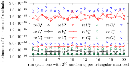
Figure 1 covers the case of upper triangular input matrices,
which can be processed by both and , and the
measures (50) and (52). Numerical
orthogonality of the singular vectors computed by is
noticeably better than of those obtained by , in the worst
case. Also, the relative SVD residuals are slightly better, in the
and the runs.
Figure 1: Numerical orthogonality of the singular vectors and the
relative SVD residuals with and on
random upper triangular double precision matrices.
Figure 2 shows the relative errors in the singular
values (51) of the same matrices from Figure 1.
The unity mark for
indicates
that can cause the relative errors in the smaller
singular values, , to be so high in the
case that their maximum was unity in all runs and cannot be
displayed in Figure 2, most likely due to underflow to zero of
when the “exact”
in (51). However, when
managed to compute the smaller singular values accurately
in the case, the maximum of their relative errors was a bit
smaller than the one from , the cause of which is worth
exploring. The same holds for the larger singular values, which were
computed accurately by both and .
Figure 2: The relative errors in the singular values with
and on random upper triangular double
precision matrices, with
and
.
To put , for
which still accurately computed all singular values (in
the exponent-“mantissa” form, and thus not underflowing), into
perspective, the highest possible condition number for triangular
matrices in the case can be estimated by recalling that
Algorithms 1 and 2 were also performed in quadruple
precision (to get , , and so ), where
and of double precision, as well as , are within
the normal range. Then, can be made small and
huge by, e.g.,
Therefore, the condition number of is a cubic expression in
, since, from (42),
Figure 3 focuses on and general input matrices,
with all their elements random. Inaccuracy of the smaller singular
values in the case motivated the search for safe exponent
ranges of the elements of input matrices that should preserve accuracy
of from for and
from for . For that, the range of
random values was restricted, and only those outputs from
rdrand for which were
accepted, where was a positive integer parameter
independently chosen for each run.
Figure 3: Numerical orthogonality of the singular vectors, the
relative SVD residuals, and the relative errors in the singular
values with on random double precision matrices, with
and
.
Figure 4 shows the results of this search for and
. Approximately half-way through the entire normal
exponent range the relative errors in the smaller singular values
stabilize to a single-digit multiple of . Thus, when for
the exponents in holds
(ignoring the exponent of ) it might be expected that
computes accurately, while should
additionally be safeguarded by its user from the elements too close to
. The proposed prescaling, but with
(or more), might be applied
to before .
Figure 4: The observed decay of the relative errors in the smaller
singular values by narrowing of the exponent range of the elements
of double precision input matrices, where
falls from for to
for , and
from to
.
A timing comparison of xLASV2 and the proposed method was not
performed since the correctly rounded routines are still in
development. By construction the proposed method is more
computationally complex than xLASV2, so it is expected to be
slower.
An unoptimized OpenMP-parallel implementation of the Kogbetliantz SVD
for of order with the scaling of in the spirit
of [22] but stronger (accounting for the two-sided
transformations of ) and the modified modulus pivot
strategy [26], when run with 64 threads spread
across the CPU cores, a deterministic reduction procedure, and
OMP_DYNAMIC=FALSE, showed up to 10% speedup over the
one-sided Jacobi SVD routine without preconditioning,
DGESVJ [27, 28], from the threaded
Intel MKL library for large enough (up to ), with the left
singular vectors from the former being a bit more orthogonal than the
ones from the latter, while the opposite was true for the right
singular vectors, on the highly conditioned input matrices
from [22]. The singular values from DGESVJ
were less than an order of magnitude more accurate.
5 Conclusions and future work
The proposed Kogbetliantz method for the SVD of order two computed
highly numerically orthogonal singular vectors in all tests. The
larger singular values were relatively accurate up to a few
in all tests, and the smaller ones were when the input
matrices were triangular, or, for the general (without zeros) input
matrices, if the range of their elements was narrower than or about
half of the width of the range of normal values.
The constituent phases of the method can be used on their own. The
prescaling might help xLASV2 when its inputs are small. The
highly accurate triangularization might be combined with
xLASV2 instead, as an alternative method for general
matrices. And the proposed SVD of triangular matrices demonstrates
some of the benefits of the more complex correctly rounded operations
(), but they go beyond that.
High relative accuracy for from (19) might
be achieved, barring underflow, if the four-way fused dot product
operation , DOT4, with a single rounding of the exact
value [29], becomes available in hardware. Then the
denominator of the expression for in (19)
could be computed, even without scaling if in a wider datatype, by the
DOT4, and the numerator by the DOT2 () operation.
The proposed heuristic for improving orthogonality of the left
singular vectors might be helpful in other cases when two plane
rotations have to be composed into one and the tangents of their
angles are known. It already brings a slight advantage to the
Kogbetliantz SVD of order with respect to the one-sided Jacobi
SVD in this regard.
With a proper vectorization, and by removing all redundancies from the
preliminary implementation, it might be feasible to speed up the
Kogbetliantz SVD of order further, since adding more threads is
beneficial as long as their number is not above .
Supplementary information.
The document sm.pdf supplements this paper with further
remarks on methods for larger matrices and the single precision
testing results.
Acknowledgments.
The author would like to thank Dean Singer for his material support
and to Vjeran Hari for fruitful discussions.
Declarations
Funding.
This work was supported in part by Croatian Science Foundation under
the expired project IP–2014–09–3670 “Matrix Factorizations and
Block Diagonalization Algorithms”
(MFBDA), in the form of
unlimited compute time granted for the testing.
Competing interests.
The author has no relevant competing interests to declare.
Anderson et al. [1999]
Anderson, E.,
Bai, Z.,
Bischof, C.,
Blackford, S.,
Demmel, J.,
Dongarra, J.,
Du Croz, J.,
Greenbaum, A.,
Hammarling, S.,
McKenney, A.,
Sorensen, D.:
LAPACK Users’ Guide,
edn.
Software, Environments and Tools.
SIAM,
Philadelphia, PA, USA
(1999).
https://doi.org/10.1137/1.9780898719604
Moler and Stewart [1973]
Moler, C.B.,
Stewart, G.W.:
An algorithm for generalized matrix eigenvalue problems.
SIAM J. Numer. Anal.
10(2),
241–256
(1973)
https://doi.org/10.1137/0710024
Demmel and Kahan [1990]
Demmel, J.,
Kahan, W.:
Accurate singular values of bidiagonal matrices.
SIAM J. Sci. Statist. Comput.
11(5),
873–912
(1990)
https://doi.org/10.1137/0911052
Charlier et al. [1987]
Charlier, J.P.,
Vanbegin, M.,
Van Dooren, P.:
On efficient implementations of Kogbetliantz’s algorithm for
computing the singular value decomposition.
Numer. Math.
52(3),
279–300
(1987)
https://doi.org/10.1007/BF01398880
Stewart [1992]
Stewart, G.W.:
An updating algorithm for subspace tracking.
IEEE Trans. Signal Process.
40(6),
1535–1541
(1992)
https://doi.org/10.1109/78.139256
Quintana-Ortí
et al. [1998]
Quintana-Ortí, G.,
Sun, X.,
Bischof, C.H.:
A BLAS-3 version of the QR factorization with column pivoting.
SIAM J. Sci. Comp.
19(5),
1486–1494
(1998)
https://doi.org/10.1137/S1064827595296732
Hari and
Matejaš [2009]
Hari, V.,
Matejaš, J.:
Accuracy of two SVD algorithms for triangular matrices.
Appl. Math. Comput.
210(1),
232–257
(2009)
https://doi.org/10.1016/j.amc.2008.12.086
Hari and
Veselić [1987]
Hari, V.,
Veselić, K.:
On Jacobi methods for singular value decompositions.
SIAM J. Sci. Statist. Comput.
8(5),
741–754
(1987)
https://doi.org/10.1137/0908064
Hari and
Zadelj-Martić [2007]
Hari, V.,
Zadelj-Martić, V.:
Parallelizing the Kogbetliantz method: A first attempt.
J. Numer. Anal. Ind. Appl. Math.
2(1–2),
49–66
(2007)
Hari [1991]
Hari, V.:
On sharp quadratic convergence bounds for the serial Jacobi
methods.
Numer. Math.
60(1),
375–406
(1991)
https://doi.org/10.1007/BF01385728
Matejaš and
Hari [2015]
Matejaš, J.,
Hari, V.:
On high relative accuracy of the Kogbetliantz method.
Linear Algebra Appl.
464,
100–129
(2015)
https://doi.org/10.1016/j.laa.2014.02.024
Novaković [2020]
Novaković, V.:
Batched computation of the singular value decompositions of order two
by the AVX-512 vectorization.
Parallel Process. Lett.
30(4),
1–232050015
(2020)
https://doi.org/10.1142/S0129626420500152
Novaković and
Singer [2022]
Novaković, V.,
Singer, S.:
A Kogbetliantz-type algorithm for the hyperbolic SVD.
Numer. Algorithms
90(2),
523–561
(2022)
https://doi.org/10.1007/s11075-021-01197-4
Bečka et al. [2002]
Bečka, M.,
Okša, G.,
Vajteršic, M.:
Dynamic ordering for a parallel block-Jacobi SVD algorithm.
Parallel Comp.
28(2),
243–262
(2002)
https://doi.org/10.1016/S0167-8191(01)00138-7
Okša et al. [2022]
Okša, G.,
Yamamoto, Y.,
Vajteršic, M.:
Convergence to singular triplets in the two-sided block-Jacobi SVD
algorithm with dynamic ordering.
SIAM J. Matrix Anal. Appl.
43(3),
1238–1262
(2022)
https://doi.org/10.1137/21M1411895
Borges [2020]
Borges, C.F.:
Algorithm 1014: An improved algorithm for hypot(x,y).
ACM Trans. Math. Softw.
47(1),
1–129
(2020)
https://doi.org/10.1145/3428446
Sibidanov et al. [2022]
Sibidanov, A.,
Zimmermann, P.,
Glondu, S.:
The CORE-MATH project.
In: 2022 IEEE Symposium on Computer Arithmetic
(ARITH),
pp. 26–34
(2022).
https://doi.org/10.1109/ARITH54963.2022.00014
Novaković [2023]
Novaković, V.:
Vectorization of a thread-parallel Jacobi singular value
decomposition method.
SIAM J. Sci. Comput.
45(3),
73–100
(2023)
https://doi.org/10.1137/22M1478847
Lauter [2017]
Lauter, C.:
An efficient software implementation of correctly rounded operations
extending FMA: and .
In: 2017 Asilomar Conference on Signals, Systems, and
Computers,
pp. 452–456
(2017).
https://doi.org/10.1109/ACSSC.2017.8335379
Hubrecht et al. [2024]
Hubrecht, T.,
Jeannerod, C.-P.,
Muller, J.-M.:
Useful applications of correctly-rounded operators of the form
.
In: 2024 IEEE Symposium on Computer Arithmetic
(ARITH),
pp. 32–39
(2024).
https://doi.org/10.1109/ARITH61463.2024.00015
Jeannerod et al. [2013]
Jeannerod, C.-P.,
Luvet, N.,
Muller, J.-M.:
Further analysis of Kahan’s algorithm for the accurate computation
of determinants.
Math. Comp.
82(284),
2245–2264
(2013)
https://doi.org/10.1090/S0025-5718-2013-02679-8
Drmač [1997]
Drmač, Z.:
Implementation of Jacobi rotations for accurate singular value
computation in floating point arithmetic.
SIAM J. Sci. Comput.
18(4),
1200–1222
(1997)
https://doi.org/10.1137/S1064827594265095
Drmač and
Veselić [2008]
Drmač, Z.,
Veselić, K.:
New fast and accurate Jacobi SVD algorithm. II.
SIAM J. Matrix Anal. Appl.
29(4),
1343–1362
(2008)
https://doi.org/10.1137/05063920X
Lutz et al. [2024]
Lutz, D.R.,
Saini, A.,
Kroes, M.,
Elmer, T.,
Valsaraju, H.:
Fused FP8 4-way dot product with scaling and FP32 accumulation.
In: 2024 IEEE Symposium on Computer Arithmetic
(ARITH),
pp. 40–47
(2024).
https://doi.org/10.1109/ARITH61463.2024.00016