Ben Gurion University of the Negev, Israel
11email: [email protected]
Arithmetic Binary Search Trees:
Static Optimality in the Matching Model
Abstract
Motivated by recent developments in optical switching and reconfigurable network design, we study dynamic binary search trees (BSTs) in the matching model. In the classical dynamic BST model, the cost of both link traversal and basic reconfiguration (rotation) is . However, in the matching model, the BST is defined by two optical switches (that represent two matchings in an abstract way), and each switch (or matching) reconfiguration cost is while a link traversal cost is still . In this work, we propose Arithmetic BST (A-BST), a simple dynamic BST algorithm that is based on dynamic Shannon-Fano-Elias coding, and show that A-BST is statically optimal for sequences of length where is the number of nodes (keys) in the tree.
Keywords:
binary search trees static optimality matching model arithmetic coding Entropy.1 Introduction
In this paper, we study one of the most classical problems in computer science, the design of efficient binary search trees (BSTs) [24]. More concretely, we are interested in Dynamic [27] or Self-Adjusting [32] binary search trees that need to serve a sequence of requests. While traditionally binary search trees are studied in the context of data-structures with a focus on memory and running time optimization, we are motivated in the physical world implementations of binary search trees and, in particular, self-adjusting networks [7].
The Matching model and Self-adjusting networks.
Self-adjusting networks, or reconfigurable networks, are communication networks that enable dynamic physical layer topologies [17, 18, 28, 9], i.e., topologies that can change over time. Recently, reconfigurable optical switching technologies have introduced an intriguing alternative to the traditional design of datacenter networks, allowing to dynamically establish direct shortcuts between communicating partners, depending on the demand [18, 21, 28, 1]. For example, such reconfigurable links could be established to support elephant flows or traffic between two racks with significant communication demands. The potential for such demand-aware optimizations is high: empirical studies show that communication traffic features both spatial and temporal locality, i.e., traffic matrices are indeed sparse and a small number of elephant flows can constitute a significant fraction of the datacenter traffic [29, 10, 3]. The main metric of interest in these networks is the flow completion time or the average packet delay, where the reconfiguration delay (aka as latency tax [20]) can be several orders of magnitude larger than the forwarding delay, i.e., milliseconds or microseconds vs. nanoseconds or less. This brings a striking contrast to the common data-structures approach where pointer forwarding and pointer changing (e.g., rotations) are of the same time order and considered as a unit cost.
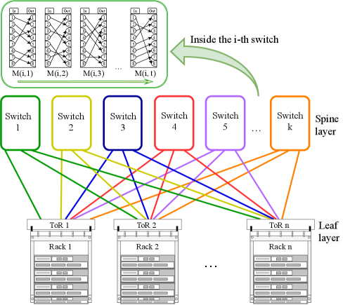
Previous work [30, 6, 5] has shown that binary search trees (and other types of trees) can be used as an important building block in the design of self-adjusting networks since they carry nice properties like local routing and low degree . Moreover, to capture many recent designs of demand-aware networks like [18, 28, 9, 17, 23], a simple leaf-spine datacenter network model called ToR-Matching-ToR (TMT) was recently proposed [4]. In the TMT model, Top of the Rack (ToR) switches (leaves) are connected via optical switches (spines), and each spine switch can have a dynamically changing matching between its input-output ports. See Figure 1 for an illustration. The exact networking and technical details of the model are out of the scope of the paper, but abstractly with only two spine switches (i.e., two matchings), the model supports a simple implementation of a dynamic binary search tree that enables a greedy routing from the root (a ToR) to any other node (ToR).
This leads to the matching model for dynamic binary search trees that we study in this paper where the tree can change at any time to any other tree but at a reconfiguration cost which is a parameter denoted as .
1.1 Formal Model and Main Result
We consider a dynamic binary search tree (BST) that needs to serve a sequence of requests from a set of unique keys, where the value of the ’th key is and the keys impose a complete order. For simplicity and w.l.o.g we assume that the keys are sorted by their value, i.e., for , (otherwise we can just rename the keys). Let be a sequence of requests for keys where .
A binary tree has a finite set of nodes with one node designated to be the root. Each node has a left and a right child which can be either a different node or a null object. Every node in , but for the root node, has a single parent node for which it is a child. We denote the root of a tree by and for a node , let and denote it left and right children. The depth of in is defined as the number of nodes on the path from the root to , denoted as . The depth of the root is therefore one.
In a binary search tree , each node has a unique key. We assume the set of nodes to be and use nodes and keys interchangeably. The tree satisfies the symmetric order condition: every node’s key is greater than the keys in its left child subtree and smaller than the keys in its right child subtree.
For a given set of keys and a sequence , the cost of the optimal static BST is defined as the BST with minimal cost to serve , formally
| (1) |
where is the set of all binary search trees.
A dynamic BST is a sequence of BSTs, with as the set of nodes. At each time step , the cost of searching (or serving) a key is , but after the request is served the BST can adjust its structure (while maintaining the symmetric order property).
The key point of this paper and in our model is that the cost assumptions differ. In previous studies, classical [8, 2, 27, 32], as well as more recent ones [16, 25, 13], to name a few, the cost of both a single link traversal and a single pointer change (usually called rotation) is units. In most of these algorithms the cost of reconfiguration of the tree is kept proportional to cost of accessing the recent key. In contrast, in the matching model the cost model assumes that any change from to is possible (it could be a single rotation or a completely new tree) but at the cost of units.
For a dynamic BST algorithm the total cost of serving starting from a BST is defined in the matching model as follows,
| (2) |
Where is the indicator function, i.e., if the event is true and 0 otherwise. From a networking perspective the cost of a dynamic BST algorithm can be seen as the total delay to serve (i.e., route) requests to nodes in from a single source that is connected to the tree’s root.
In static optimality, which we next define, we want the dynamic BST algorithm to (asymptotically) perform well even in hindsight compared to the best static tree.
Definition 1 (Static Optimality)
Let be the cost of an optimal static BST with perfect knowledge of the demand , and let On be an online algorithm for dynamic BST. We say that On is statically optimal if there exists some constant , and for any sufficiently long sequence of keys , we have that
where is the initial BST from which On starts. In other words, On’s cost is at most a constant factor higher than in the worst case.
Note that when known algorithms for dynamic BST that are static optimal, e.g., [8, 27, 32, 16, 15], can be used to achieve static optimality in our model. The more interesting scenario is when and naive current algorithms with rotation cost (or splay to the root, or move to root) of will not be static optimal. In this work, we assume for simplicity that .
Let be the number of appearances of key in up to time . Note that . For short let . Let be the frequency (or empirical) distribution of , i.e., , and the frequency distribution up to time . It is a classical result that the optimal static BST for has amortized access cost of where is the entropy function [26], i.e., .
The main result of this paper is a simple dynamic BST algorithm, A-BST, that is based on arithmetic coding [34] and in particular on a dynamic Shannon-Fano-Elias coding [14] and is statically optimal for sequences of length . Formally,
Theorem 1
A-BST (Algorithm 3) is a statically optimal, dynamic BST for sequences of length at least .
The rest of the paper is organized as follows: In Section 2 we review related concepts like Entropy and the Shannon-Fano-Elias (SFE) coding with a detailed example. Section 3 presents A-BST including related algorithms and an example for its dynamic operation. In Section 4 we prove Theorem 1. Finally, we conclude with a discussion and open questions in Section 5.
2 Preliminaries
Entropy and Shannon-Fano-Elias (SFE) Coding.
Entropy is a known measure of unpredictability of information content [31]. For a discrete random variable with possible values , the (binary) entropy of is defined as where is the probability that takes the value . Note that, and we usually assume that . Let denote ’s probability distribution, then we may write instead of .
Shannon-Fano-Elias (SFE) [14] is a well-known symbol, prefix code for lossless data compression and is the predecessor of the more famous and used (variable block length) arithmetic coding [34]. The Shannon-Fano-Elias code produce variable-length code-words based on the probability of each possible symbol. As in other entropy encoding methods (e.g., Huffman), higher probability symbols are represented using fewer bits, to reduce the expected code length. Unlike Huffman coding the coding method works for any order of symbols and the probabilities do not need to be sorted. This will fit better with the searching property we need in the tree later on.
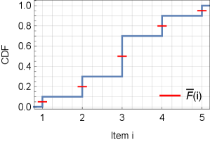
The encoding is based on the cumulative distribution function (CDF) of the probability distribution,
| (3) |
and encodes symbols using the function where
| (4) |
Denote by the binary representation of . The code-word for the ’th symbol consists of the first bits of the fractional part of , denoted as
| (5) |
where the code length is defined as
| (6) |
The above construction guarantees that the code-words are prefix-free and therefore appear as leaves in the binary tree that represent the code, and that the average code length ,
| (7) |
is close to the entropy of the random variable , and in particular,
| (8) |
| Example A | Example B |
 |
 |
| (a) | (e) |
 |
 |
| (b) | (f) |
 |
 |
| (c) | (g) |
 |
 |
| (d) | (h) |
For an illustration consider Example A in Figure 2 which we will use also later in the paper. Let be a random variable with five possible symbols and the corresponding probabilities . Figure 2 (a) provides the detailed parameters for the encoding of each symbol , including , the binary representation , the code-word length and the (prefix-free) binary code-word . Additionally, Figure 2 (b) presents and graphically and Figure 2 (c) shows a binary tree with leaves as the code-words where the path from the root to each leaf represent its (prefix-free) code-word. Figure 2 (d) shows the conversion of the prefix tree to a binary search tree which we will discuss next.
3 Arithmetic Binary Search Trees (A-BST)
The idea of arithmetic binary search trees is simple in principle. It is composed of three phases:
-
1.
Use arithmetic coding, and in particular, Shannon-Fano-Elias coding to create an efficient, variable-length, prefix-free code for a given (empirical) distribution.
-
2.
In turn, convert the binary tree of the prefix-free code to a biased binary search tree (with an entropy bound on its performance).
-
3.
Dynamically update the empirical distribution, the prefix-free code and the corresponding binary search tree.
We first describe steps and that may be of independent interest and then the crux of the method which is the dynamic update process.
3.1 From Shannon-Fano-Elias (SFE) coding to BST
Algorithms 1 and 2 shows how to create a near optimal biased BST for a given distribution via SFE coding. Algorithm SFE-2-BST (Algorithm 1) is first provided with a probability distribution for the biased BST. Note that, w.l.o.g, the distribution is sorted by the keys values. From the algorithm then creates a prefix-free binary code using SFE coding111Any other coding method that preserves the keys order can be used, e.g., Shannon–Fano coding [14] which split the probabilities to half, Alphabetic Codes [35] or Mehlhorn tree [26], but not e.g., Huffman coding [22], that needs to sort the probabilities. and the corresponding binary tree where keys (symbols) are at the leaves and ordered by their value (and not by probabilities). Next, the algorithm calls Algorithm PrefixTree-2-BST (Algorithm 2) which converts to a BST .
Algorithm 2 is a recursive algorithm that receives a binary tree with keys as leaves in increasing order. It creates a BST by setting the root of the tree as the key which is closer to the root between the two keys that are pre-order and post-order to the root (and then deleting the key from ). The left and right subtrees of ’s root are created by calling recursively the algorithm with the relevant subtrees of .
Recall Figure 2 (c) which shows a binary tree for the SFE code of the probability distribution in Example A. The keys are leaves and in sorted order. This tree is an intermediate result of SFE-2-BST() algorithm. Figure 2 (d) presents the corresponding BST after calling PrefixTree-2-BST. Initially is selected as the root as it is closer to the root between keys and . Then (after deleting from the tree), the algorithm continues recursively, by building the children of ’s root with the left and right subtrees of ’s root. On the left, 2 is selected as the next root and then 1 as its left child. On the right is selected as the next root and then 5 as its right child.
We can easily bound the depth of any key in the tree generated by SFE-2-BST.
Claim 1
For a key-sorted probability distribution , the algorithm SFE-2-BST() creates a biased BST where for each key it holds .
Proof
The SFE code creates code-words with length , so the tree in Algorithm SFE-2-BST has the leaves at depth . Algorithm PrefixTree-2-BST() does not change the symmetric order of keys that are initially stored at leaves, and can only decrease the depth of any key. ∎
We next discuss how to make the BST dynamic.
3.2 Dynamic BST
Algorithm 3 provides a pseudo-code for a dynamic Arithmetic Binary Search Tree (A-BST) . The algorithm starts from which is a balanced BST over the possible keys (assuming no knowledge on the keys distribution). The algorithm maintains two probability distribution vectors that change over time, and . holds the probability distribution by which the current BST was built and initially is set to the uniform distribution. holds the empirical distribution of up to time and is updated on each request, i.e., 222To avoid zero probabilities, in practice is set by Laplace rule [12] to be , this does not change the main Theorem since for we have . For simplicity of exposition we assume .. The crux of the algorithm is that, whenever a key is requested, if as a result , then is updated to be equal to , and a new BST is created (at cost of ) from . Note that upon a request to key only increases while all other probabilities decrease. So the condition can only become valid for when key is requested.
We demonstrate the algorithm using Example B. Assume we have keys and after the first ten requests in we have . Note that this is the empirical distribution of Example A, so is the BST that is shown in Figure 2 (d). Next we assume that the and requests are for key 1. After the request and so and remains as . After the request we have and , and now . So at time , a new SFE code and a new BST are created with the empirical distribution . The details of the code for this distribution are given in Figure 2 (e)-(g) and the new BST, is shown in Figure 2 (h). Note that key 1 got closer to the root.
Next we analyse A-BST and show it is statically optimal.
4 A-BST is statically Optimal
We now prove the main result of this work. Recall that we assume and the more intresting case is .
Theorem 4.1
A-BST (Algorithm 3) is a statically optimal, dynamic BST for sequences of length at least .
Proof
Let be the BST tree of the algorithm at time . Let be the probability distribution by which was build. Let be the frequency distribution of up to time . Note that . Observe that Algorithm 3 guarantees that for each and each we have . We first analyse the searching cost (or access cost [11]), of Algorithm 3.
Next we consider the cost and analyze each key at a time. We follow an idea mentioned in a classical paper on dynamic Huffman coding by Vitter [33] and is due to a personal communication of Vitter with B. Chazelle. Consider the last requests for key . For each such request, since , we have . So the sum of these requests is at most .
Similarly for each ’th request of key where where , and the cost of all of these requests is less than . So for each key
| (13) | ||||
| (14) | ||||
| (15) | ||||
| (16) |
From this it follows that:
| (17) | ||||
| (18) |
A result identical to Eq. (18) was recently shown in [19]. Next we consider the adjustment cost. We do it again, one key at a time. For a key consider all the adjustment it caused (lines 5-6 in Algorithm 3). We consider two cases: i) all adjustment when and ii) . To prove these two cases we will use the following claim.
Claim 2
Let be the key that cause an adjustment (lines 5-6 in Algorithm 3) at time . Let be the time of the previous adjustment initiated by any key. Then .
Proof
By Algorithm 3 after the adjustment at time , was set to and in particular was set to . The result follows since at time we have
| (19) |
∎
We can now analyse the two adjustment cases.
Case i: .
First notice that if then for each . Assume a time for which and lines 5-6 in Algorithm 3 was executed. Now consider time where the previous execution of lines 5-6 occurred.
From Claim 2 and using the assumption that , the number of requests to key since the last adjustment is:
| (20) |
Therefore we can amortize the adjustment at time (of cost ) with the (at least) cost of the adversary accessing the (at least) requests to key between and .
Case ii: .
From Claim 2, at least doubles between each adjustment that is caused by key . So until , key can cause at most adjustments at a total adjustment cost that is less than .
It follows that the adjustment cost, , of Algorithm 3 can be bounded as follows:
| (21) | ||||
| (22) | ||||
| (23) | ||||
| (24) |
Equations (22) and (23) follows from cases (i) and (ii) above. Eq. (24) follows form the assumption that .
To finalize the proof we combine the above results to find the cost of A-BST.
| (25) | ||||
| (26) | ||||
| (27) |
∎
5 Discussion and Open Questions
We believe that the matching model brings some interesting research directions. Our model can emulate the standard BST model when , while dynamic optimally is a major and a long-standing open question for this case [32], it may be possible that for some range of the question becomes easier. Another property, possibly simpler, to prove or disprove approximation for, is a working-set like theorem [32]. A nice feature of the matching model is that it supports more complex networks than a BST. It is a future research direction to prove static optimality and other online properties for such networks.
Regarding A-BST, the algorithm can be extended in several directions to be more adaptive. First, it can work with a (memory) window instead of the whole history to become more dynamic. Careful attention is required to decide the window size in order not to lose the static optimally feature. More generally, as in arithmetic coding [14] which is an extension of the SFE coding, the prediction model can be independently replaced by a more sophisticated model than the current Laplace model.
References
- [1] Alistarh, D., Ballani, H., Costa, P., Funnell, A., Benjamin, J., Watts, P., Thomsen, B.: A high-radix, low-latency optical switch for data centers. In: Proceedings of the 2015 ACM conference on SIGCOMM. pp. 367–368 (2015)
- [2] Allen, B., Munro, I.: Self-organizing binary search trees. Journal of the ACM (JACM) 25(4), 526–535 (1978)
- [3] Avin, C., Ghobadi, M., Griner, C., Schmid, S.: On the complexity of traffic traces and implications. Proceedings of the ACM on Measurement and Analysis of Computing Systems 4(1), 1–29 (2020)
- [4] Avin, C., Griner, C., Salem, I., Schmid, S.: An online matching model for self-adjusting tor-to-tor networks. arXiv preprint arXiv:2006.11148 (2020)
- [5] Avin, C., Mondal, K., Schmid, S.: Demand-aware network designs of bounded degree. Distributed Computing pp. 1–15 (2017)
- [6] Avin, C., Schmid, S.: Renets: Toward statically optimal self-adjusting networks. arXiv preprint arXiv:1904.03263. To appear in APOCS 2020. (2019)
- [7] Avin, C., Schmid, S.: Toward demand-aware networking: A theory for self-adjusting networks. ACM SIGCOMM Computer Communication Review 48(5), 31–40 (2019)
- [8] Baer, J.L.: Weight-balanced trees. In: Proceedings of the May 19-22, 1975, national computer conference and exposition. pp. 467–472 (1975)
- [9] Ballani, H., Costa, P., Behrendt, R., Cletheroe, D., Haller, I., Jozwik, K., Karinou, F., Lange, S., Shi, K., Thomsen, B., et al.: Sirius: A flat datacenter network with nanosecond optical switching. In: Proceedings of the 2016 ACM SIGCOMM Conference. pp. 782–797 (2020)
- [10] Benson, T., Anand, A., Akella, A., Zhang, M.: Understanding data center traffic characteristics. In: Proc. 1st ACM Workshop on Research on Enterprise Networking (WREN). pp. 65–72. ACM (2009)
- [11] Blum, A., Chawla, S., Kalai, A.T.: Static optimality and dynamic search-optimality in lists and trees. Algorithmica 36 (2016)
- [12] Carnap, R.: On the application of inductive logic. Philosophy and phenomenological research 8(1), 133–148 (1947)
- [13] Chalermsook, P., Jiamjitrak, W.P.: New binary search tree bounds via geometric inversions. In: 28th Annual European Symposium on Algorithms (ESA 2020). Schloss Dagstuhl-Leibniz-Zentrum für Informatik (2020)
- [14] Cover, T.M., Thomas, J.A.: Elements of information theory. John Wiley & Sons (2012)
- [15] Demaine, E.D., Harmon, D., Iacono, J., Kane, D., Pătraşcu, M.: The geometry of binary search trees. In: Proceedings of the twentieth annual ACM-SIAM symposium on Discrete algorithms. pp. 496–505. SIAM (2009)
- [16] Demaine, E.D., Harmon, D., Iacono, J., Pătraşcu, M.: Dynamic optimality—almost. SIAM Journal on Computing 37(1), 240–251 (2007)
- [17] Farrington, N., Porter, G., Radhakrishnan, S., Bazzaz, H.H., Subramanya, V., Fainman, Y., Papen, G., Vahdat, A.: Helios: a hybrid electrical/optical switch architecture for modular data centers. In: Proceedings of the ACM SIGCOMM 2010 conference. pp. 339–350 (2010)
- [18] Ghobadi, M., Mahajan, R., Phanishayee, A., Devanur, N., Kulkarni, J., Ranade, G., Blanche, P.A., Rastegarfar, H., Glick, M., Kilper, D.: Projector: Agile reconfigurable data center interconnect. In: Proceedings of the 2016 ACM SIGCOMM Conference. pp. 216–229 (2016)
- [19] Golin, M., Iacono, J., Langerman, S., Munro, J.I., Nekrich, Y.: Dynamic Trees with Almost-Optimal Access Cost. In: Azar, Y., Bast, H., Herman, G. (eds.) 26th Annual European Symposium on Algorithms (ESA 2018). Leibniz International Proceedings in Informatics (LIPIcs), vol. 112, pp. 38:1–38:14. Schloss Dagstuhl–Leibniz-Zentrum fuer Informatik, Dagstuhl, Germany (2018). https://doi.org/10.4230/LIPIcs.ESA.2018.38, http://drops.dagstuhl.de/opus/volltexte/2018/9501
- [20] Griner, C., Zerwas, J., Blenk, A., Ghobadi, M., Schmid, S., Avin, C.: Performance analysis of demand-oblivious and demand-aware optical datacenter network designs. arXiv preprint arXiv:2010.13081. (2020)
- [21] Hamedazimi, N., Qazi, Z., Gupta, H., Sekar, V., Das, S.R., Longtin, J.P., Shah, H., Tanwer, A.: Firefly: A reconfigurable wireless data center fabric using free-space optics. In: Proceedings of the 2014 ACM conference on SIGCOMM. pp. 319–330 (2014)
- [22] Huffman, D.A.: A method for the construction of minimum-redundancy codes. Proceedings of the IRE 40(9), 1098–1101 (1952)
- [23] Kassing, S., Valadarsky, A., Shahaf, G., Schapira, M., Singla, A.: Beyond fat-trees without antennae, mirrors, and disco-balls. In: Proceedings of the 2017 ACM conference on SIGCOMM. pp. 281–294. ACM (2017)
- [24] Knuth, D.E.: Optimum binary search trees. Acta informatica 1(1), 14–25 (1971)
- [25] Levy, C., Tarjan, R.: A new path from splay to dynamic optimality. In: Proceedings of the Thirtieth Annual ACM-SIAM Symposium on Discrete Algorithms. pp. 1311–1330. SIAM (2019)
- [26] Mehlhorn, K.: Nearly optimal binary search trees. Acta Informatica 5(4), 287–295 (1975)
- [27] Mehlhorn, K.: Dynamic binary search. SIAM Journal on Computing 8(2), 175–198 (1979)
- [28] Mellette, W.M., McGuinness, R., Roy, A., Forencich, A., Papen, G., Snoeren, A.C., Porter, G.: Rotornet: A scalable, low-complexity, optical datacenter network. In: Proceedings of the 2016 ACM SIGCOMM Conference. pp. 267–280 (2017)
- [29] Roy, A., Zeng, H., Bagga, J., Porter, G., Snoeren, A.C.: Inside the social network’s (datacenter) network. In: Proc. ACM SIGCOMM Computer Communication Review (CCR). vol. 45, pp. 123–137. ACM (2015)
- [30] Schmid, S., Avin, C., Scheideler, C., Borokhovich, M., Haeupler, B., Lotker, Z.: Splaynet: Towards locally self-adjusting networks. IEEE/ACM Transactions on Networking 24(3), 1421–1433 (2015)
- [31] Shannon, C.E.: A mathematical theory of communication. The Bell system technical journal 27(3), 379–423 (1948)
- [32] Sleator, D.D., Tarjan, R.E.: Self-adjusting binary search trees. Journal of the ACM (JACM) 32(3), 652–686 (1985)
- [33] Vitter, J.S.: Design and analysis of dynamic huffman codes. Journal of the ACM (JACM) 34(4), 825–845 (1987)
- [34] Witten, I.H., Neal, R.M., Cleary, J.G.: Arithmetic coding for data compression. Commun. ACM 30(6), 520–540 (Jun 1987). https://doi.org/10.1145/214762.214771, http://doi.acm.org/10.1145/214762.214771
- [35] Yeung, R.W.: Alphabetic codes revisited. IEEE Transactions on Information Theory 37(3), 564–572 (1991)