Arbitrary high-order structure-preserving methods for the quantum Zakharov system

Gengen Zhang [email protected] Chaolong Jiang [email protected] School of Mathematics and Statistics, Yunnan University, Kunming 650504, China School of Statistics and Mathematics, Yunnan University of Finance and Economics, Kunming 650221, China

Abstract

In this paper, we present a new methodology to develop arbitrary high-order structure-preserving methods for solving the quantum Zakharov system. The key ingredients of our method are: (i) the original Hamiltonian energy is reformulated into a quadratic form by introducing a new quadratic auxiliary variable; (ii) based on the energy variational principle, the original system is then rewritten into a new equivalent system which inherits the mass conservation law and a quadratic energy; (iii) the resulting system is discretized by symplectic Runge-Kutta method in time combining with the Fourier pseudo-spectral method in space. The proposed method achieves arbitrary high-order accurate in time and can preserve the discrete mass and original Hamiltonian energy exactly. Moreover, an efficient iterative solver is presented to solve the resulting discrete nonlinear equations. Finally, ample numerical examples are presented to demonstrate the theoretical claims and illustrate the efficiency of our methods.

keywords:

Quantum Zakharov system; symplectic Runge-Kutta method; structure-preserving method; Fourier pseudo-spectral method.

1 Introduction

The quantum Zakharov system [20, 27] is widely used to describe the nonlinear interaction between the Langmuir waves and the ion-acoustic waves. In this paper, we consider the following quantum Zakharov system (QZS):

\left\{\begin{split}&{\rm i}\partial_{t}E({\bf x},t)+\Delta E({\bf x},t)-\varepsilon^{2}\Delta^{2}E({\bf x},t)=N({\bf x},t)E({\bf x},t),\\ &\partial_{tt}N({\bf x},t)-\Delta N({\bf x},t)+\varepsilon^{2}\Delta^{2}N({\bf x},t)=\Delta|E({\bf x},t)|^{2},\ {\bf x}\in\Omega,\ 0<t\leq T,\\ &E({\bf x},0)=E_{0}({\bf x}),\ N({\bf x},0)=N_{0}({\bf x}),\ N_{t}({\bf x},0)=N_{1}({\bf x}),\ {\bf x}\in\bar{\Omega}\subset\mathbb{R}^{d},\ d=1,2,\end{split}\right.

(1.1)

where $\text{i}=\sqrt{-1}$ is the complex unit, $t$ is the time variable, ${\bf x}$ is the spatial variable, the complex-valued function $E:=E({\bf x},t)$ denotes the slowly varying envelope of the rapidly oscillatory electric field, the real-valued function $N:=N({\bf x},t)$ represents the low-frequency variation of the density of the ions, $\Delta$ is the usual Laplace operator, the quantum effect $\varepsilon>0$ is the ratio of the ion plasma and the temperature of electrons, and $E_{0}(\mathbf{x})$ , $N_{0}(\mathbf{x})$ and $N_{1}(\mathbf{x})$ are given initial conditions, and $N_{1}(\mathbf{x})$ satisfies the following compatibility condition [8, 22]:

\int_{\Omega}N_{1}(\mathbf{x})d\mathbf{x}=0.

(1.2)

In the special case $\varepsilon=0$ , it reduces to the classical Zakharov system (ZS), which have been widely applied to various physical problems, such as plasmas [25, 56], hydrodynamics [15], the theory of molecular chains [14] and so on. When either the electrons temperature is low or the ion-plasma frequency is high, the quantum effect can be characterized by the fourth-order perturbation with a quantum parameter $\varepsilon$ . For more details, please refer to Refs. [26, 38, 41]. With the periodic boundary condition, the QZS (1.1) conserves the mass

\begin{split}&\mathcal{M}(t)=\int_{\Omega}|E|^{2}d{\bf x}\equiv\mathcal{M}(0),\ t\geq 0,\end{split}

(1.3)

and the energy

\begin{split}&\mathcal{H}(t)=\int_{\Omega}\left(\left|\nabla E\right|^{2}+\frac{1}{2}(|\nabla v|^{2}+N^{2})+\varepsilon^{2}\left|\triangle E\right|^{2}+\frac{\varepsilon^{2}}{2}\left|\nabla N\right|^{2}+N|E|^{2}\right)d{\bf x}\equiv\mathcal{H}(0),\ t\geq 0,\end{split}

(1.4)

where $\triangle v=N_{t}$ .

Extensive mathematical and numerical studies have been carried out for the above QZS (1.1) in the literature. Along the mathematical front, Fang et al. [18] showed that the QZS (1.1) is locally well-posed in $L^{2}(\mathbb{R}^{d})$ data for dimension up to eight, together with global existence for dimensions up to five, which is different from the classical ZS where the global and local well-posedness of the Cauchy problem is known only for $1\leq d\leq 3$ [17, 21]. The blow-up in finite time of the solution for high-dimensional classical ZS was investigated in [39]. Along the numerical front, the numerical studies of the classical or generalized ZS are very rich, such as time splitting methods [3, 2, 33, 34], scalar auxiliary variable approach [49], finite difference methods [1, 9, 22, 54], discontinuous Galerkin method [53], etc. Recently, there has been growing interest in developing accurate and efficient numerical methods for the QZS (1.1). Baumstark and Schratz [5] developed a new class of asymptotic preserving trigonometric integrators for the QZS (1.1). Meanwhile, it is shown rigorously in mathematics that the scheme converges to the classical ZS in the limit $\varepsilon\rightarrow 0$ uniformly in the time discretization parameter. Zhang [58] proposed an explicit mass-conserving time-splitting exponential wave integrator Fourier pseudo-spectral (TS-EWI-FP) method for the QZS (1.1). However, these mentioned schemes cannot conserve the energy (1.4) of the QZS (1.1). It has been shown that in the numerical simulation of the collision of solitons, the solution of mass- and energy-conserving schemes cannot produce nonlinear blow-up [45, 57]. Later on, Zhang and Su [59] proposed and analyzed a linearly-implicit conservative compact finite difference method for the QZS (1.1). Cai et al. [8] proposed a novel of mass- and energy-conserving compact finite difference scheme for the QZS (1.1). However it is shown rigorously in mathematics that these existing mass- and energy-conserving schemes are only second-order accurate in time. In [13, 24, 31], it is clear to observe that high-order accurate structure-preserving scheme will provide much smaller numerical error and more robust than the second-order accurate one as the large time step is chosen. Thus, it is desirable to propose high-order accurate mass- and energy-preserving methods for solving the QZS (1.1).

As a matter of the fact, in the past few decades, how to devise high-order accurate energy-preserving schemes for conservative systems have attracted plenty of attention. The excellent ones include Hamiltonian Boundary Value Methods (HBVMs) [6, 7], energy-preserving variant of collocation methods [12, 28], high-order averaged vector field (AVF) methods [35, 43, 40], functionally fitted energy-preserving methods [42, 37, 52] and energy-preserving continuous stage Runge-Kutta (RK) methods [42, 50], etc. These methods can be easily extended to propose high-order accurate energy-preserving scheme for the QZS (1.1), which however cannot preserve the mass exactly [4, 36]. Based on the basic principle of the structure-preserving method where the numerical method should preserve the intrinsic properties of the original problems as much as possible, it is valuable to expect that the high-order mass and energy-preserving discretizations for the QZS (1.1) will produce richer information on the continuous system. Very recently, inspired by the ideas of the invariant energy quadratization (IEQ) approach [55], a new class of high-order accurate energy-preserving methods are proposed in [11, 23], which was generalized more recently by Tapley[51]. Especially, the term “quadratic auxiliary variable (QAV) approach” was coined by Gong et al. in [11]. The key differences between the IEQ approach and the QAV approach are: (i) the auxiliary variable introduced by the QAV approach shall be quadratic; (ii) as a high-order quadratic invariant-preserving method in time is applied to the equivalent system, the resulting method can not only preserve the original Hamiltonian energy instead of a modified energy [19, 30, 32], but also the original quadratic invariants of the equivalent system. Thus, the QAV approach will be an efficient strategy to develop high-order accurate mass- and energy-preserving scheme for the QZS (1.1), however to our knowledge, there has been no reference considering this issue.

In this paper, motivated by the QAV approach, we first introduce a quadratic auxiliary variable to transform the Hamiltonian energy into a quadratic from, and the original system is then reformulated into a new equivalent system. Finally, a fully-discrete method is obtained by using the RK method in time and the Fourier pseudo-spectral method in space for the reformulated system. We show that when the symplectic RK method is selected, the proposed method can conserve the discrete mass and original Hamiltonian energy exactly. In addition, to solve the discrete nonlinear equations of our method efficiently, an efficient fixed-pointed iteration method is proposed.

The rest of the paper is organized as follows. In section 2, we first reformulate the original QZS (1.1) into an equivalent form, and the energy conservation law and the mass conservation law of the reformulated system are then investigated. In section 3, a new class of high-order structure-preserving schemes are proposed based on the symplectic RK method in time and the Fourier pseudo-spectral method in space, respectively. In Section 4, an efficient implementention for the proposed scheme is presented. In Section 5, extensive numerical experiments for the QZS (1.1) are carried out to illustrate the capability and accuracy of the method, and show some complex dynamical behaviors. Finally, some conclusions are drawn in Section 6.

2 Model reformulation

Denote $u=(E,N,v)^{T}$ , the QZS (1.1) can be written into the following energy-conserving system

\displaystyle\begin{split}\partial_{t}u=S\frac{\delta\mathcal{H}}{\delta\bar{u}},\end{split}

(2.1)

where $\bar{u}$ is the complex conjugate of $u$ ,

\displaystyle S=\left(\begin{array}[]{ccc}{\rm i}&0&0\\ 0&0&1\\ 0&-1&0\end{array}\right)

is the skew-adjoint operator, and the Hamiltonian energy functional

\mathcal{H}[u]=\int_{\Omega}\left(-\left|\nabla E\right|^{2}-\frac{1}{2}\left(|\nabla v|^{2}+N^{2}\right)-\varepsilon^{2}\left|\Delta E\right|^{2}-\frac{\varepsilon^{2}}{2}\left|\nabla N\right|^{2}-N|E|^{2}\right)d{\bf x}.

(2.2)

Next, based on the idea of the QAV approach, we first introduce a quadratic auxiliary variable, as follows:

q:=q({\bf x},t)=|E|^{2},

(2.3)

the original energy (2.2) is then transformed into the following quadratic form

\mathcal{E}[u,q]=\int_{\Omega}\left(-\left|\nabla E\right|^{2}-\frac{1}{2}\left(|\nabla v|^{2}+N^{2}\right)-\varepsilon^{2}\left|\Delta E\right|^{2}-\frac{\varepsilon^{2}}{2}\left|\nabla N\right|^{2}-Nq\right)d{\bf x}.

(2.4)

According to the energy variational principle, we rewritten the QZS (2.1) into a new equivalent system

\begin{cases}E_{t}={\rm i}(\Delta E-\varepsilon^{2}\Delta^{2}E-NE),\\ N_{t}=\Delta v,\\ v_{t}=N-\varepsilon^{2}\Delta N+q,\\ q_{t}=2{\rm Re}(E_{t}\cdot\bar{E}),\\ \end{cases}

(2.5)

with the consistent initial conditions

		$\displaystyle E({\bf x},0)=E_{0}({\bf x}),\ N({\bf x},0)=N_{0}({\bf x}),\ q({\bf x},0)=\big{\|}E_{0}({\bf x})\big{\|}^{2},\ N_{t}({\bf x},0)=N_{1}({\bf x}),$
		$\displaystyle\Delta v({\bf x},0)=N_{1}({\bf x}),\ \int_{\Omega}v(\mathbf{x},0)d\mathbf{x}=0,\ {\bf x}\in\bar{\Omega},$		(2.6)

where ${\rm Re}(\bullet)$ represents the real part of $\bullet$ , and we impose $\int_{\Omega}v(\mathbf{x},0)d\mathbf{x}=0$ in the equivalent form so that $v(\mathbf{x},t)$ is uniquely defined in the second equality of (2.5)[8].

Subsequently, we focus on investigating the structure-preserving properties of the reformulated system (2.5)-(2).

Theorem 2.1.

Under the periodic boundary conditions, the system (2.5)-(2) possesses the following conservation laws:

•

The mass

$\displaystyle\mathcal{M}(t)\equiv\mathcal{M}(0),\ t\geq 0,$ (2.7)

where $\mathcal{M}(t)$ is defined by (1.3).

•

The two quadratic invariants

		$\displaystyle q({\bf x},t)-\|E({\bf x},t)\|^{2}=q({\bf x},0)-\|E({\bf x},0)\|^{2}\equiv 0,\ {\bf x}\in\Omega,\;t\geq 0,$		(2.8)
		$\displaystyle\mathcal{E}(t)\equiv\mathcal{E}(0),\ t\geq 0,$		(2.9)

where $\mathcal{E}(t)$ are defined by (2.4).

Proof.

We make the inner product of the first equation of (2.5) with $E$ and then take the real part of the resulting equation to obtain

\frac{\mathrm{d}}{\mathrm{d}t}(|E|^{2},1)=2{\rm Re}\int_{\Omega}{\rm i}\left(-\left|\nabla E\right|^{2}-\varepsilon^{2}\left|\Delta E\right|^{2}-N|E|^{2}\right)d{\bf x}=0,

(2.10)

which implies that the system (2.5) satisfies (2.7).

Combining the initial condition $q({\bf x},0)=|E({\bf x},0)|^{2}$ with the fourth equation of the system (2.5), we can deduce

\partial_{t}(q-|E({\bf x},t)|^{2})=0,

which yields (2.8).

Using the periodic boundary condition and the system (2.5), we then obtain

	$\displaystyle\frac{\mathrm{d}}{\mathrm{d}t}\mathcal{E}(t)$	$\displaystyle=2{\rm Re}(\Delta E,E_{t})-2\varepsilon^{2}{\rm Re}(\Delta^{2}E,E_{t})-2{\rm Re}(NE,E_{t})-(N,N_{t})+\varepsilon^{2}(\Delta N,N_{t})-(q,N_{t})+(v_{t},N_{t})$
		$\displaystyle=2{\rm Re}\left(\Delta E-\varepsilon^{2}\Delta^{2}E-NE,E_{t}\right)+\left(-N+\varepsilon^{2}\Delta N-q+v_{t},N_{t}\right)$
		$\displaystyle=2{\rm Re}\left(-{\rm i}E_{t},E_{t}\right)$
		$\displaystyle=0,$

where $(f,g)=\int_{\Omega}f\bar{g}\mathrm{d}{\bf x}$ , for any $f,g\in L^{2}(\Omega)$ is denoted as the continuous $L^{2}$ inner product. This completes the proof. ∎

3 High-order accurate mass- and energy-preserving methods

In this section, the symplectic RK methods are first used to discretize the system (2.5) in time and a class of semi-discrete RK method is proposed, which can conserve the mass and original Hamiltonian energy of the QZS (1.1). Subsequently, the Fourier pseudo-spectral method is then employed to discretize the spatial variables of the semi-discrete scheme and a class of fully-discrete high-order mass- and energy-preserving scheme are presented.

3.1 Time semi-discretization

Let the time step $\tau=\frac{T}{J}$ and denote $t_{n}=n\tau$ for $0\leq n\leq J$ . Let $w^{n}$ and $w_{ni}$ be the numerical approximations of the function $w({\bf x},t)$ at $t_{n}$ and $t_{n}+c_{i}\tau$ , respectively. Applying an $s$ -stage RK method to discrete the system (2.5) in time and the following semi-discrete scheme is presented.

Scheme 3.1.

Let $b_{i},a_{ij}({i,j=1,\cdots,s})$ be real numbers and let $c_{i}=\sum_{j=1}^{s}a_{ij}$ . For given $(E^{n},N^{n},v^{n},q^{n})$ , an $s$ -stage RK method is given by

\begin{cases}E_{ni}=E^{n}+\tau\sum\limits_{j=1}^{s}a_{ij}k_{j}^{1},\ k_{i}^{1}={\rm i}(\Delta E_{ni}-\varepsilon^{2}\Delta^{2}E_{ni}-N_{ni}E_{ni}),\\ N_{ni}=N^{n}+\tau\sum\limits_{j=1}^{s}a_{ij}k_{j}^{2},\ k_{i}^{2}=\Delta v_{ni},\\ v_{ni}=v^{n}+\tau\sum\limits_{j=1}^{s}a_{ij}k_{j}^{3},\ k_{i}^{3}=N_{ni}-\varepsilon^{2}\Delta N_{ni}+Q_{ni},\\ Q_{ni}=q^{n}+\tau\sum\limits_{j=1}^{s}a_{ij}k_{j}^{4},\ k_{i}^{4}=2{\rm Re}(\bar{E}_{ni}\cdot k_{i}^{1}).\end{cases}

(3.1)

Then $(E^{n+1},N^{n+1},v^{n+1},q^{n+1})$ is updated by

$\displaystyle E^{n+1}$	$\displaystyle=E^{n}+\tau\sum\limits_{i=1}^{s}b_{i}k_{i}^{1},$	(3.2)
$\displaystyle N^{n+1}$	$\displaystyle=N^{n}+\tau\sum\limits_{i=1}^{s}b_{i}k_{i}^{2},$	(3.3)
$\displaystyle v^{n+1}$	$\displaystyle=v^{n}+\tau\sum\limits_{i=1}^{s}b_{i}k_{i}^{3},$	(3.4)
$\displaystyle q^{n+1}$	$\displaystyle=q^{n}+\tau\sum\limits_{i=1}^{s}b_{i}k_{i}^{4}.$	(3.5)

Theorem 3.2.

If the coefficients of the RK method (3.1) satisfy

b_{i}a_{ij}+b_{j}a_{ji}=b_{i}b_{j},\quad\forall~{}i,j=1,\cdots,s,

(3.6)

and the periodic boundary condition is considered, the Scheme 3.1 preserves the following semi-discrete conservation laws

•

The semi-discrete mass

$\displaystyle\mathcal{M}^{n+1}=\mathcal{M}^{n},\ \mathcal{M}^{n}=\big{(}|E^{n}|^{2},1\big{)},\ n=0,1,2,\cdots,J.$ (3.7)

•

The two semi-discrete quadratic invariants

		$\displaystyle q^{n}-\|E^{n}\|^{2}=0,$		(3.8)
		$\displaystyle\mathcal{E}^{n+1}=\mathcal{E}^{n},\ n=0,1,2,\cdots,J,$		(3.9)

where

\displaystyle\mathcal{E}^{n}=(\Delta E^{n},E^{n})-\varepsilon^{2}(\Delta E^{n},\Delta E^{n})-\frac{1}{2}(N^{n},N^{n})+\frac{\varepsilon^{2}}{2}(\Delta N^{n},N^{n})-(N^{n},q^{n})+\frac{1}{2}(\Delta v^{n},v^{n}).

Proof.

According to Eq. (3.2), we have

\begin{array}[]{lll}\mathcal{M}^{n+1}=\mathcal{M}^{n}+\tau\sum\limits_{i=1}^{s}b_{i}\big{(}k_{i}^{1},E^{n}\big{)}+\tau\sum\limits_{i=1}^{s}b_{i}\big{(}E^{n},k_{i}^{1}\big{)}+\tau^{2}\sum\limits_{i,j=1}^{s}b_{i}b_{j}\big{(}k_{i}^{1},k_{j}^{1}\big{)}.\end{array}

(3.10)

Plugging $E^{n}=E_{ni}-\tau\sum\limits_{j=1}^{s}a_{ij}k_{j}^{1}$ into the right hand side of (3.10) and using (3.6), we have

\mathcal{M}^{n+1}=\mathcal{M}^{n}+\tau\sum\limits_{i=1}^{s}b_{i}\big{(}E_{ni},k_{i}^{1}\big{)}+\tau\sum\limits_{i=1}^{s}b_{i}\big{(}k_{i}^{1},E_{ni}\big{)}.

(3.11)

Furthermore, we can deduce

	$\displaystyle\tau\sum\limits_{i=1}^{s}b_{i}\big{(}E_{ni},k_{i}^{1}\big{)}$	$\displaystyle+\tau\sum\limits_{i=1}^{s}b_{i}\big{(}k_{i}^{1},E_{ni}\big{)}$
		$\displaystyle=2\tau\sum\limits_{i=1}^{s}b_{i}{\rm Re}(k_{i}^{1},\bar{E}_{ni})$
		$\displaystyle=2\tau\sum\limits_{i=1}^{s}b_{i}{\rm Re}\Big{(}{\rm i}(\Delta E_{ni}-\varepsilon^{2}\Delta^{2}E_{ni}-N_{ni}E_{ni}),\bar{E}_{ni}\Big{)}$
		$\displaystyle=2\tau\sum\limits_{i=1}^{s}b_{i}{\rm Re}\Big{(}{\rm i}\big{(}-\|\nabla E_{ni}\|^{2}-\varepsilon^{2}\|\Delta E_{ni}\|^{2}-N_{ni}\|E_{ni}\|^{2}\big{)},1\Big{)}$
		$\displaystyle=0.$

Then, combining the above equation with (3.11), we obtain the discrete mass conservation law (3.7).

Based on (3.2), (3.6) and $E^{n}=E_{ni}-\tau\sum\limits_{j=1}^{s}a_{ij}k_{j}^{1}$ , we get

$\displaystyle\|E^{n+1}\|^{2}-\|E^{n}\|^{2}$	$\displaystyle=E^{n+1}\cdot\bar{E}^{n+1}-E^{n}\cdot\bar{E}^{n}$
	$\displaystyle=\tau\sum\limits_{i=1}^{s}b_{i}(k_{i}^{1}\cdot\bar{E}^{n})+\tau\sum\limits_{i=1}^{s}b_{i}(\overline{k}_{i}^{1}\cdot E^{n})+\tau^{2}\sum\limits_{i,j=1}^{s}b_{i}b_{j}(k_{i}^{1}\cdot\bar{k}_{j}^{1})$
	$\displaystyle=\tau\sum\limits_{i=1}^{s}b_{i}(k_{i}^{1}\cdot\bar{E}_{ni})+\tau\sum\limits_{i=1}^{s}b_{i}(\bar{k}_{i}^{1}\cdot E_{ni})+\tau^{2}\sum\limits_{i,j=1}^{s}(-b_{i}a_{ij}-b_{j}a_{ji}+b_{i}b_{j})(k_{i}^{1}\cdot\bar{k}_{j}^{1})$
	$\displaystyle=\tau\sum\limits_{i=1}^{s}b_{i}(k_{i}^{1}\cdot\bar{E}_{ni})+\tau\sum\limits_{i=1}^{s}b_{i}(\bar{k}_{i}^{1}\cdot E_{ni}).$	(3.12)

Noticing that

\begin{array}[]{lll}q^{n+1}-q^{n}=\tau\sum\limits_{i=1}^{s}b_{i}k_{i}^{4}=2\tau\sum\limits_{i=1}^{s}b_{i}{\rm Re}(k_{i}^{1}\cdot\bar{E}_{ni})=\tau\sum\limits_{i=1}^{s}b_{i}(k_{i}^{1}\cdot\bar{E}_{ni})+\tau\sum\limits_{i=1}^{s}b_{i}(\bar{k}_{i}^{1}\cdot E_{ni}).\end{array}

(3.13)

It follows from (3.12) and (3.13) that

\displaystyle q^{n+1}-|E^{n+1}|^{2}=q^{n}-|E^{n}|^{2}.

(3.14)

With the help of the initial condition $q^{0}=|E^{0}|^{2}$ , we can obtain (3.8).

Similar to Eq. (3.11), we can obtain from the Scheme 3.1 that

	$\displaystyle(\Delta E^{n+1},E^{n+1})-(\Delta E^{n},E^{n})=2\tau\sum\limits_{i=1}^{s}b_{i}{\rm Re}\big{(}k_{i}^{1},\Delta E_{ni}\big{)},$
	$\displaystyle(\Delta E^{n+1},\Delta E^{n+1})-(\Delta E^{n},\Delta E^{n})=2\tau\sum\limits_{i=1}^{s}b_{i}{\rm Re}\big{(}k_{i}^{1},\Delta^{2}E_{ni}\big{)},$
	$\displaystyle(N^{n+1},N^{n+1})-(N^{n},N^{n})=2\tau\sum\limits_{i=1}^{s}b_{i}\big{(}N_{ni},k_{i}^{2}\big{)},$
	$\displaystyle(\Delta N^{n+1},N^{n+1})-(\Delta N^{n},N^{n})=2\tau\sum\limits_{i=1}^{s}b_{i}\big{(}\Delta N_{ni},k_{i}^{2}\big{)},$
	$\displaystyle(N^{n+1},q^{n+1})-(N^{n},q^{n})=\tau\sum\limits_{i=1}^{s}b_{i}\left[\big{(}k_{i}^{2},Q_{ni}\big{)}+\big{(}N_{ni},k_{i}^{4}\big{)}\right],$
	$\displaystyle(\Delta v^{n+1},v^{n+1})-(\Delta v^{n},v^{n})=2\tau\sum\limits_{i=1}^{s}b_{i}\big{(}\Delta v_{ni},k_{i}^{3}\big{)}.$

Thus, together with (3.1), we can derive

	$\displaystyle\mathcal{E}^{n+1}-\mathcal{E}^{n}$	$\displaystyle=\tau\sum\limits_{i=1}^{s}b_{i}\left[2{\rm Re}\big{(}k_{i}^{1},\Delta E_{ni}\big{)}-2\varepsilon^{2}{\rm Re}\big{(}k_{i}^{1},\Delta^{2}E_{ni}\big{)}-\big{(}N_{ni},k_{i}^{2}\big{)}\right.$
		$\displaystyle~{}~{}~{}\left.+\varepsilon^{2}\big{(}\Delta N_{ni},k_{i}^{2}\big{)}-\big{(}N_{ni},k_{i}^{4}\big{)}-\big{(}k_{i}^{2},Q_{ni}\big{)}+\big{(}\Delta v_{ni},k_{i}^{3}\big{)}\right]$
		$\displaystyle=\tau\sum\limits_{i=1}^{s}b_{i}\left[2{\rm Re}\big{(}k_{i}^{1},\Delta E_{ni}-\varepsilon^{2}\Delta^{2}E_{ni}-N_{ni}E_{ni}\big{)}-\big{(}N_{ni}-\varepsilon^{2}\Delta N_{ni}+Q_{ni}-k_{i}^{3},k_{i}^{2}\big{)}\right]$
		$\displaystyle=\tau\sum\limits_{i=1}^{s}b_{i}\left[2{\rm Re}\big{(}k_{i}^{1},-{\rm i}k_{i}^{1}\big{)}-\big{(}N_{ni}-\varepsilon^{2}\Delta N_{ni}+Q_{ni}-k_{i}^{3},k_{i}^{2}\big{)}\right]$
		$\displaystyle=0,$

which implies that the Scheme 3.1 satisfies (3.9). ∎

Theorem 3.3.

Under the consistent initial condition (2), the periodic boundary condition and the condition (3.6), the Scheme 3.1 conserves the original Hamiltonian energy at each time step, as follows:

\mathcal{H}^{n}\equiv\mathcal{H}^{0},\ n=1,2,\cdots,J,

(3.15)

where

\displaystyle\mathcal{H}^{n}=(\Delta E^{n},E^{n})-\varepsilon^{2}(\Delta E^{n},\Delta E^{n})-\frac{1}{2}(N^{n},N^{n})+\frac{\varepsilon^{2}}{2}(\Delta N^{n},N^{n})-(N^{n},|E^{n}|^{2})+\frac{1}{2}(\Delta v^{n},v^{n}).

Proof.

As the consistent initial condition (2), the periodic boundary condition and the condition (3.6) are considered, we can obtain from Theorem 3.2 that

q^{n}=|E^{n}|^{2},\ n=0,1,2,\cdots,J,

(3.16)

and

\mathcal{E}^{n+1}=\mathcal{E}^{n},\ \ n=0,1,2,\cdots,J,

(3.17)

where

\displaystyle\mathcal{E}^{n}=(\Delta E^{n},E^{n})-\varepsilon^{2}(\Delta E^{n},\Delta E^{n})-\frac{1}{2}(N^{n},N^{n})+\frac{\varepsilon^{2}}{2}(\Delta N^{n},N^{n})-(N^{n},q^{n})+\frac{1}{2}(\Delta v^{n},v^{n}).

Then substituting (3.16) into (3.17), we obtain (3.15). We finish the proof. ∎

Scheme 3.2.

As the symplectic RK method is selected, the Scheme 3.1 is equivalent to the following s-stage RK (using (3.8) of Theorem 3.2):

\begin{cases}E_{ni}=E^{n}+\tau\sum\limits_{j=1}^{s}a_{ij}k_{j}^{1},\\ k_{i}^{1}={\rm i}(\Delta E_{ni}-\varepsilon^{2}\Delta^{2}E_{ni}-N_{ni}E_{ni}),\\ N_{ni}=N^{n}+\tau\sum\limits_{j=1}^{s}a_{ij}k_{j}^{2},\\ k_{i}^{2}=\Delta v_{ni},\\ v_{ni}=v^{n}+\tau\sum\limits_{j=1}^{s}a_{ij}k_{j}^{3},\\ k_{i}^{3}=N_{ni}-\varepsilon^{2}\Delta N_{ni}+|E^{n}|^{2}+2\tau\sum\limits_{j=1}^{s}a_{ij}{\rm Re}(\bar{E}_{nj}\cdot k_{j}^{1}),\end{cases}

(3.18)

where $(E^{n+1},N^{n+1},v^{n+1})$ is obtained by

	$\displaystyle E^{n+1}=E^{n}+\tau\sum\limits_{i=1}^{s}b_{i}k_{i}^{1},$
	$\displaystyle N^{n+1}=N^{n}+\tau\sum\limits_{i=1}^{s}b_{i}k_{i}^{2},$
	$\displaystyle v^{n+1}=v^{n}+\tau\sum\limits_{i=1}^{s}b_{i}k_{i}^{3},$

which implies that the QAV approach need introduce an auxiliary variable, but the auxiliary variable can be eliminated in practical computations. Thus, it cannot increase additional computational costs.

Remark 3.1.

We should note that the Gauss method where the RK coefficients $c_{1},c_{2},\cdots,c_{s}$ are chosen as the Gaussian quadrature nodes, i.e., the zeros of the $s$ -th shifted Legendre polynomial $\frac{d^{s}}{dx^{s}}(x^{s}(x-1)^{s})$ satisfies the condition (3.6) [29]. In particular, the coefficients of the Gauss methods of order 2, 4 and 6 can be given[29, 44], respectively, (see Table. 1).

${c}$	${A}$
	${b}^{T}$

= $\frac{1}{2}$ $\frac{1}{2}$ 1 , ${c}$ ${A}$ ${b}^{T}$ = $\frac{1}{2}-\frac{\sqrt{3}}{6}$ $\frac{1}{4}$ $\frac{1}{4}-\frac{\sqrt{3}}{6}$ $\frac{1}{2}+\frac{\sqrt{3}}{6}$ $\frac{1}{4}+\frac{\sqrt{3}}{6}$ $\frac{1}{4}$ $\frac{1}{2}$ $\frac{1}{2}$ ,
${c}$ ${A}$ ${b}^{T}$ = $\frac{1}{2}-\frac{\sqrt{15}}{10}$ $\frac{5}{36}$ $\frac{2}{9}-\frac{\sqrt{15}}{15}$ $\frac{5}{36}-\frac{\sqrt{15}}{30}$ $\frac{1}{2}$ $\frac{5}{36}+\frac{\sqrt{15}}{24}$ $\frac{2}{9}$ $\frac{5}{36}-\frac{\sqrt{15}}{24}$ $\frac{1}{2}+\frac{\sqrt{15}}{10}$ $\frac{5}{36}+\frac{\sqrt{15}}{30}$ $\frac{2}{9}+\frac{\sqrt{15}}{15}$ $\frac{5}{36}$ $\frac{5}{18}$ $\frac{4}{9}$ $\frac{5}{18}$ .

Table 1: The Gauss methods of 2 (s=1), 4 (s=2) and 6 (s=3).

Remark 3.2.

If the Gauss method of order 2 (see Table. 1) is selected, the Scheme 3.2 reduced to the following semi-discrete Crank-Nicolson scheme (CNS)[8]

\left\{\begin{split}&{\rm i}\delta_{t}E^{n}+\Delta E^{n+\frac{1}{2}}-\varepsilon^{2}\Delta^{2}E^{n+\frac{1}{2}}-N^{n+\frac{1}{2}}E^{n+\frac{1}{2}}=0,\\ &\delta_{t}N^{n}=\Delta v^{n+\frac{1}{2}},\\ &\delta_{t}v^{n}-N^{n+\frac{1}{2}}+\varepsilon^{2}\Delta N^{n+\frac{1}{2}}-\frac{1}{2}(|E^{n+1}|^{2}+|E^{n}|^{2})=0,\ n=0,1,2,\cdots,J,\\ \end{split}\right.

(3.19)

where

\displaystyle\delta_{t}w^{n}=\frac{w^{n+1}-w^{n}}{\tau},\ w^{n+\frac{1}{2}}=\frac{w^{n+1}+w^{n}}{2}.

Remark 3.3.

It is well-known that the scalar auxiliary variable (SAV) approach [47, 48] is also an efficient method for developing high-order accurate structure-preserving methods for the conservative systems [13, 31]. However, we should note that it is challenging for introducing a special scalar auxiliary variable to construct high-order accurate methods in time which can preserve the original Hamiltonian energy of the system.

3.2 Full discretization

In this subsection, the Fourier pseudo-spectral method is employed to discretize the Scheme 3.2 in spatial variables and a class of fully discrete structure-preserving schemes are presented.

Let the domain $\Omega=[a,b)\times[c,d)$ be uniformly partition with spatial steps $h_{x}=\frac{b-a}{\mathcal{N}_{x}}$ and $h_{y}=\frac{d-c}{\mathcal{N}_{y}}$ , where $\mathcal{N}_{x}$ and $\mathcal{N}_{y}$ are two positive even integers. Then, we denote the spatial grid points as

\displaystyle\Omega_{h}=\{(x_{j},y_{k})|x_{j}=a+jh_{x},\ y_{k}=c+kh_{y},\ 0\leq j\leq\mathcal{N}_{x}-1,\ 0\leq k\leq\mathcal{N}_{y}-1\}.

Let $w_{j,k}$ be the numerical approximation of $w(x_{j},y_{k},t)$ on $\Omega_{h}$ , and denote

w:=(w_{0,0},w_{1,0},\cdots,w_{\mathcal{N}_{x}-1,0},w_{0,1},w_{1,1},\cdots,w_{\mathcal{N}_{x}-1,1},\cdots,w_{0,\mathcal{N}_{y}-1},w_{1,\mathcal{N}_{y}-1},\cdots,w_{\mathcal{N}_{x}-1,\mathcal{N}_{y}-1})^{T}

be the solution vector; we also define discrete inner product and norms as

\displaystyle\langle u,w\rangle_{h}=h_{x}h_{y}\sum\limits_{j=0}^{\mathcal{N_{x}}-1}\sum\limits_{k=0}^{\mathcal{N}_{y}-1}u_{j,k}{{{\bar{w}}}}_{j,k},\ \ \ \|w\|_{h}=\langle w,w\rangle_{h}^{\frac{1}{2}},\ \ \|w\|_{h,{\infty}}=\max\limits_{(x_{j},y_{k})\in\Omega_{h}}|w_{j,k}|.

In addition, we denote $`\cdot$ ’ as the element-wise product of vectors ${u}$ and ${w}$ , that is

\displaystyle u\cdot w=

\displaystyle\big{(}u_{0,0}w_{0,0},\cdots,u_{\mathcal{N}_{x}-1,0}w_{\mathcal{N}_{x}-1,0},\cdots,u_{0,\mathcal{N}_{y}-1}w_{0,\mathcal{N}_{y}-1},\cdots,u_{\mathcal{N}_{x}-1,\mathcal{N}_{y}-1}w_{\mathcal{N}_{x}-1,\mathcal{N}_{y}-1}\big{)}^{T}.

For brevity, we denote ${w}\cdot w$ and ${w}\cdot\bar{w}$ as ${w}^{2}$ and $|w|^{2}$ , respectively.

Let ${X}_{j}(x)$ and ${Y}_{k}(y)$ be the interpolation basis functions given by

\displaystyle{X}_{i}(x)=\frac{1}{\mathcal{N}_{x}}\sum\limits_{m={-\mathcal{N}_{x}}/{2}}^{{\mathcal{N}_{x}}/{2}}\frac{1}{a_{m}}e^{\text{i}m\mu_{x}(x-x_{i})},\ {Y}_{j}(y)=\frac{1}{\mathcal{N}_{y}}\sum\limits_{m={-\mathcal{N}_{y}}/{2}}^{{\mathcal{N}_{y}}/{2}}\frac{1}{b_{m}}e^{\text{i}m\mu_{y}(y-y_{j})},

where $\mu_{x}=\frac{2\pi}{b-a},\ \mu_{y}=\frac{2\pi}{d-c}$ , $a_{m}=\left\{\begin{array}[]{lll}1,&\mid m\mid<\frac{\mathcal{N}_{x}}{2},\vspace{2mm}\\ 2,&\mid m\mid=\frac{\mathcal{N}_{x}}{2}.\end{array}\right.$ and $b_{m}=\left\{\begin{array}[]{lll}1,&\mid m\mid<\frac{\mathcal{N}_{y}}{2},\vspace{2mm}\\ 2,&\mid m\mid=\frac{\mathcal{N}_{y}}{2}.\end{array}\right.$ Then, we define $\mathcal{S}^{{}^{\prime\prime}}$ as the interpolation space

\displaystyle\mathcal{S}^{{}^{\prime\prime}}={\rm span}\big{\{}{X}_{j}(x){Y}_{k}(y)|~{}0\leq j\leq\mathcal{N}_{x}-1,\ 0\leq j\leq\mathcal{N}_{y}-1\big{\}},

and the interpolation operator $I_{\mathbb{N}}:C(\Omega)\rightarrow\mathcal{S}^{{}^{\prime\prime}}$ is given by [10]

\displaystyle I_{\mathbb{N}}w(x,y,t)=\sum\limits_{j=0}^{\mathcal{N}_{x}-1}\sum\limits_{j=0}^{\mathcal{N}_{y}-1}w(x_{j},y_{k},t){X}_{j}(x){Y}_{k}(y).

(3.20)

Taking the second-order derivative with respect to $x$ and $y$ , respectively and the resulting expression at the collocation points $w(x_{j},y_{k},t)$ reads

		$\displaystyle\frac{\partial^{2}}{\partial x^{2}}I_{\mathbb{N}}w(x_{j},y_{k},t)=\sum_{l=0}^{\mathcal{N}_{x}-1}w(x_{j},y_{k},t)\frac{d^{2}}{dx^{2}}{X}_{l}(x_{j})=\sum_{l=0}^{\mathcal{N}_{x}-1}(\mathbf{D}_{2}^{x})_{j,l}w(x_{j},y_{k},t),$		(3.21)
		$\displaystyle\frac{\partial^{2}}{\partial y^{2}}I_{\mathbb{N}}w(x_{j},y_{k},t)=\sum_{l=0}^{\mathcal{N}_{y}-1}w(x_{j},y_{k},t)\frac{d^{2}}{dy^{2}}{Y}_{l}(y_{k})=\sum_{l=0}^{\mathcal{N}_{y}-1}w(x_{j},y_{k},t)(\mathbf{D}_{2}^{y})_{k,l},$		(3.22)

where [10]

	$\displaystyle(\mathbf{D}_{2}^{x})_{j,k}=\left\{\begin{array}[]{lll}\frac{1}{2}\mu^{2}_{x}(-1)^{j+k+1}\csc^{2}\big{(}\mu_{x}\frac{x_{j}-x_{k}}{2}\big{)},&j\neq k,\\ -\mu^{2}_{x}\frac{\mathcal{N}_{x}^{2}+2}{12},&j=k,\end{array}\right.$
	$\displaystyle(\mathbf{D}_{2}^{y})_{j,k}=\left\{\begin{array}[]{lll}\frac{1}{2}\mu^{2}_{y}(-1)^{j+k+1}\csc^{2}\big{(}\mu_{y}\frac{y_{j}-y_{k}}{2}\big{)},&j\neq k,\\ \\ -\mu^{2}_{y}\frac{\mathcal{N}_{y}^{2}+2}{12},&j=k.\end{array}\right.$

Lemma 3.1.

For the matrix $\mathbf{D}_{2}^{\theta}$ ( $\theta=x$ or $y$ ), there exists the following relation [46]

\displaystyle\mathbf{D}_{2}^{\theta}=\mathcal{F}_{\mathcal{N}_{\theta}}^{H}\Lambda_{\theta}\mathcal{F}_{\mathcal{N}_{\theta}},

(3.23)

where $\mathcal{F}_{\mathcal{N}_{\theta}}$ denotes the discrete Fourier transform (DFT) matrix, and satisfies $\mathcal{F}_{\mathcal{N}_{\theta}}^{H}$ is the conjugate transpose matrix of $\mathcal{F}_{\mathcal{N}_{\theta}}$ ,

\displaystyle\Lambda_{\theta}=-\mu_{\theta}^{2}\text{diag}\big{[}0^{2},1^{2},\cdots,(\frac{\mathcal{N_{\theta}}}{2})^{2},(-\frac{\mathcal{N_{\theta}}}{2}+1)^{2},\cdots,(-2)^{2},(-1)^{2}\big{]}.

(3.24)

Then, applying the Fourier pseudo-spectral method to the Scheme 3.2, we obtain the following fully discrete scheme.

Scheme 3.3.

Let $b_{i},a_{ij}({i,j=1,\cdots,s})$ be real numbers and let $c_{i}=\sum_{j=1}^{s}a_{ij}$ . For given $(E^{n},N^{n},v^{n})$ , an $s$ -stage RK Fourier pseudo-spectral method is given by

\begin{cases}E_{ni}=E^{n}+\tau\sum\limits_{j=1}^{s}a_{ij}k_{j}^{1},\\ k_{i}^{1}={\rm i}(\Delta_{h}E_{ni}-\varepsilon^{2}\Delta_{h}^{2}E_{ni}-N_{ni}\cdot E_{ni}),\\ N_{ni}=N^{n}+\tau\sum\limits_{j=1}^{s}a_{ij}k_{j}^{2},\\ k_{i}^{2}=\Delta_{h}v_{ni},\\ v_{ni}=v^{n}+\tau\sum\limits_{j=1}^{s}a_{ij}k_{j}^{3},\\ k_{i}^{3}=N_{ni}-\varepsilon^{2}\Delta_{h}N_{ni}+|E^{n}|^{2}+2\tau\sum\limits_{j=1}^{s}a_{ij}{\rm Re}(\bar{E}_{nj}\cdot k_{j}^{1}),\end{cases}

(3.25)

where $\Delta_{h}=\mathbf{I}_{y}\otimes\mathbf{D}_{x}^{2}+\mathbf{D}_{y}^{2}\otimes\mathbf{I}_{x}$ . Then $(E^{n+1},N^{n+1},v^{n+1})$ is updated by

	$\displaystyle E^{n+1}=E^{n}+\tau\sum\limits_{i=1}^{s}b_{i}k_{i}^{1},$		(3.26)
	$\displaystyle N^{n+1}=N^{n}+\tau\sum\limits_{i=1}^{s}b_{i}k_{i}^{2},$		(3.27)
	$\displaystyle v^{n+1}=v^{n}+\tau\sum\limits_{i=1}^{s}b_{i}k_{i}^{3},$		(3.28)

with the initial conditions

\displaystyle E^{0}=E_{0}({\bf x}),\ N^{0}=N_{0}({\bf x}),\ \Delta_{h}v^{0}=N_{1}({\bf x}).

(3.29)

We note that based on the condition $\int_{\Omega}v(\mathbf{x},0)d\mathbf{x}=0$ , we can obtain the zeroth Fourier coefficient on $v^{0}$ is zero, so that the Poisson equation $\Delta_{h}v^{0}=N_{1}({\bf x})$ with periodic boundary conditions only has a unique solution.

For the Scheme 3.3, we can obtain the following theorem which can be carried out similarly as Theorem 3.2 and Theorem 3.3, respectively.

Theorem 3.4.

If the RK coefficients of the Scheme 3.3 satisfy the condition (3.6), then Scheme 3.3 satisfies the following discrete conservative properties

•

The discrete mass

$\displaystyle\mathcal{M}_{h}^{n+1}=\mathcal{M}_{h}^{n},\ \mathcal{M}_{h}^{n}=\big{\langle}E^{n},E^{n}\big{\rangle}_{h},\ n=0,1,2,\cdots,J.$ (3.30)
•

The discrete quadratic invariant

$\displaystyle q^{n}-|E^{n}|^{2}={\bf 0},\ n=0,1,2,\cdots,J.$ (3.31)

•

The discrete Hamiltonian energy

\displaystyle\mathcal{H}_{h}^{n+1}=\mathcal{H}_{h}^{n},\ n=0,1,2,\cdots,J,

(3.32)

where

	$\displaystyle\mathcal{H}_{h}^{n}=$	$\displaystyle\langle\Delta_{h}E^{n},E^{n}\rangle_{h}-\varepsilon^{2}\langle\Delta_{h}E^{n},\Delta_{h}E^{n}\rangle_{h}$
		$\displaystyle-\frac{1}{2}\langle N^{n},N^{n}\rangle_{h}+\frac{\varepsilon^{2}}{2}\langle\Delta_{h}N^{n},N^{n}\rangle_{h}-\langle N^{n},\|E^{n}\|^{n}\rangle_{h}+\frac{1}{2}\langle\Delta_{h}v^{n},v^{n}\rangle_{h}.$

4 An efficient implementation for the proposed scheme

In this section, we will present an efficient fixed point iteration method to solve the resulting nonlinear equations of the Scheme 3.3, which is mainly based on the matrix diagonalization method (see Ref. [46] and references therein) and the discrete Fourier transform algorithm. For simplicity, we only consider the one dimensional QZS (1.1) and generalizations to two dimensional case is straightforward for tensor product grids and the results remain valid with modifications. In addition, we only take the 2-stage Gauss method (i.e., $s=2$ ) as an example in which the RK coefficients $a_{ij},\ b_{i}\ (i,j=1,2,\cdots,s)$ are given in Table 1.

For given $E^{n},\ N^{n}$ and $v^{n}$ , 2-stage Gauss method is equivalent to

	$\displaystyle k_{1}^{1}=\text{i}(\Delta_{h}-\varepsilon^{2}\Delta_{h}^{2})E_{n1}-\text{i}N_{n1}\cdot E_{n1},\quad k_{2}^{1}=\text{i}(\Delta_{h}-\varepsilon^{2}\Delta_{h}^{2})E_{n2}-\text{i}N_{n2}\cdot E_{n2},$		(4.1)
	$\displaystyle k_{1}^{2}=\Delta_{h}v_{n1},\hskip 113.81102ptk_{2}^{2}=\Delta_{h}v_{n2},$		(4.2)
	$\displaystyle k_{1}^{3}=(1-\varepsilon^{2}\Delta_{h})N_{n1}+Q_{1},\hskip 52.63777ptk_{2}^{3}=(1-\varepsilon^{2}\Delta_{h})N_{n2}+Q_{2},$		(4.3)
	$\displaystyle E_{n1}=E^{n}+\tau a_{11}k_{1}^{1}+\tau a_{12}k_{2}^{1},\hskip 34.14322ptE_{n2}=E^{n}+\tau a_{21}k_{1}^{1}+\tau a_{22}k_{2}^{1},$		(4.4)
	$\displaystyle N_{n1}=N^{n}+\tau a_{11}k_{1}^{2}+\tau a_{12}k_{2}^{2},\hskip 32.72049ptN_{n2}=N^{n}+\tau a_{21}k_{1}^{2}+\tau a_{22}k_{2}^{2},$		(4.5)
	$\displaystyle v_{n1}=v^{n}+\tau a_{11}k_{1}^{3}+\tau a_{12}k_{2}^{3},\hskip 42.67912ptv_{n2}=v^{n}+\tau a_{21}k_{1}^{3}+\tau a_{22}k_{2}^{3},$		(4.6)

where

	$\displaystyle Q_{1}=\|E^{n}\|^{2}+\tau a_{11}k_{1}^{4}+\tau a_{12}k_{2}^{4},\ Q_{2}=\|E^{n}\|^{2}+\tau a_{21}k_{1}^{4}+\tau a_{22}k_{2}^{4},$		(4.7)
	$\displaystyle k_{1}^{4}=2\text{Re}(\bar{E}_{n1}\cdot k_{1}^{1}),~{}~{}~{}~{}~{}~{}\hskip 34.14322ptk_{2}^{4}=2\text{Re}(\bar{E}_{n2}\cdot k_{2}^{1}).$		(4.8)

Then, $E^{n+1},\ N^{n+1}$ and $v^{n+1}$ are obtained by

		$\displaystyle E^{n+1}=E^{n}+\tau b_{1}k_{1}^{1}+\tau b_{2}k_{2}^{1},\ N^{n+1}=N^{n}+\tau b_{1}k_{1}^{2}+\tau b_{2}k_{2}^{2},$		(4.9)
		$\displaystyle v^{n+1}=v^{n}+\tau b_{1}k_{1}^{3}+\tau b_{2}k_{2}^{3}.$		(4.10)

With (4.1) and (4.4), we have

		$\displaystyle\left[\begin{array}[]{cc}\vspace{2mm}1-\tau\text{i}(\Delta_{h}-\varepsilon^{2}\Delta_{h}^{2})a_{11}&-\tau\text{i}(\Delta_{h}-\varepsilon^{2}\Delta_{h}^{2})a_{12}\\ -\tau\text{i}(\Delta_{h}-\varepsilon^{2}\Delta_{h}^{2})a_{21}&1-\tau\text{i}(\Delta_{h}-\varepsilon^{2}\Delta_{h}^{2})a_{22}\\ \end{array}\right]\left[\begin{array}[]{c}\vspace{2mm}k_{1}^{1}\\ k_{2}^{1}\end{array}\right]$		(4.15)
		$\displaystyle~{}~{}~{}~{}~{}~{}~{}~{}~{}~{}~{}~{}~{}~{}~{}~{}~{}~{}~{}~{}~{}~{}~{}~{}~{}~{}~{}~{}~{}~{}~{}~{}~{}~{}~{}~{}~{}~{}~{}~{}~{}~{}~{}~{}~{}~{}~{}~{}~{}~{}~{}~{}~{}~{}~{}~{}~{}~{}~{}=\left[\begin{array}[]{c}\vspace{2mm}\text{i}(\Delta_{h}-\varepsilon^{2}\Delta_{h}^{2})E^{n}-\text{i}N_{n1}\cdot E_{n1}\\ \text{i}(\Delta_{h}-\varepsilon^{2}\Delta_{h}^{2})E^{n}-\text{i}N_{n2}\cdot E_{n2}\end{array}\right].$		(4.18)

Analogously, we can obtain from (4.2)-(4.3) and (4.5)-(4.6) that

		$\displaystyle\left[\begin{array}[]{cc}\vspace{2mm}1-\tau^{2}(a_{11}^{2}+a_{12}a_{21})(\Delta_{h}-\varepsilon^{2}\Delta_{h}^{2})&-\tau^{2}(a_{11}a_{12}+a_{12}a_{22})(\Delta_{h}-\varepsilon^{2}\Delta_{h}^{2})\\ -\tau^{2}(a_{21}a_{11}+a_{22}a_{21})(\Delta_{h}-\varepsilon^{2}\Delta_{h}^{2})&1-\tau^{2}(a_{21}a_{12}+a_{22}^{2})(\Delta_{h}-\varepsilon^{2}\Delta_{h}^{2})\\ \end{array}\right]\left[\begin{array}[]{c}\vspace{2mm}k_{1}^{2}\\ k_{2}^{2}\end{array}\right]$		(4.23)
		$\displaystyle~{}~{}~{}~{}~{}~{}~{}~{}~{}~{}~{}~{}~{}~{}~{}~{}~{}~{}~{}~{}~{}~{}~{}~{}~{}~{}~{}~{}~{}~{}=\left[\begin{array}[]{c}\vspace{2mm}\tau(a_{11}+a_{12})(\Delta_{h}-\varepsilon^{2}\Delta_{h}^{2})N^{n}+\Delta_{h}v^{n}+\tau a_{11}\Delta_{h}Q_{1}+\tau a_{12}\Delta_{h}Q_{2}\\ \tau(a_{21}+a_{22})(\Delta_{h}-\varepsilon^{2}\Delta_{h}^{2})N^{n}+\Delta_{h}v^{n}+\tau a_{21}\Delta_{h}Q_{1}+\tau a_{22}\Delta_{h}Q_{2}\end{array}\right].$		(4.26)

It is clear to see that if $k_{i}^{1}$ and $k_{i}^{2}\ (i=1,2)$ are obtained after solving the nonlinear equations (4.18) and (4.26), respectively, and $E_{ni}\ (i=1,2)$ and $N_{ni}\ (i=1,2)$ are updated by (4.4) and (4.5), respectively. Subsequently, $k_{i}^{3}\ (i=1,2)$ and $k_{i}^{4}\ (i=1,2)$ are updated by (4.3) and (4.8), respectively. Thus, for the 2-stage Gauss method, we only need to solve the nonlinear equations (4.18) and (4.26), respectively. For the nonlinear algebraic equations (4.18) and (4.26), we apply the following fixed-point iteration strategy,

	$\displaystyle\left[\begin{array}[]{cc}\vspace{2mm}1-\tau\text{i}(\Delta_{h}-\varepsilon^{2}\Delta_{h}^{2})a_{11}&-\tau\text{i}(\Delta_{h}-\varepsilon^{2}\Delta_{h}^{2})a_{12}\\ -\tau\text{i}(\Delta_{h}-\varepsilon^{2}\Delta_{h}^{2})a_{21}&1-\tau\text{i}(\Delta_{h}-\varepsilon^{2}\Delta_{h}^{2})a_{22}\\ \end{array}\right]\left[\begin{array}[]{c}\vspace{2mm}(k_{1}^{1})^{l+1}\\ (k_{2}^{1})^{l+1}\end{array}\right]$
	$\displaystyle~{}~{}~{}~{}~{}~{}~{}~{}~{}~{}~{}~{}~{}~{}~{}~{}~{}~{}~{}~{}~{}~{}~{}~{}~{}~{}~{}~{}~{}~{}~{}~{}~{}~{}~{}~{}~{}~{}~{}~{}~{}~{}~{}~{}~{}~{}~{}~{}~{}~{}~{}~{}~{}~{}~{}~{}~{}~{}~{}~{}~{}~{}~{}~{}~{}~{}~{}~{}~{}~{}~{}~{}~{}~{}~{}~{}~{}~{}~{}~{}=\left[\begin{array}[]{c}\vspace{2mm}\text{i}(\Delta_{h}-\varepsilon^{2}\Delta_{h}^{2})E^{n}-\text{i}N_{n1}^{l}\cdot E_{n1}^{l}\\ \text{i}(\Delta_{h}-\varepsilon^{2}\Delta_{h}^{2})E^{n}-\text{i}N_{n2}^{l}\cdot E_{n2}^{l}\end{array}\right],$

and

	$\displaystyle\left[\begin{array}[]{cc}\vspace{2mm}1-\tau^{2}(a_{11}^{2}+a_{12}a_{21})(\Delta_{h}-\varepsilon^{2}\Delta_{h}^{2})&-\tau^{2}(a_{11}a_{12}+a_{12}a_{22})(\Delta_{h}-\varepsilon^{2}\Delta_{h}^{2})\\ -\tau^{2}(a_{21}a_{11}+a_{22}a_{21})(\Delta_{h}-\varepsilon^{2}\Delta_{h}^{2})&1-\tau^{2}(a_{21}a_{12}+a_{22}^{2})(\Delta_{h}-\varepsilon^{2}\Delta_{h}^{2})\\ \end{array}\right]\left[\begin{array}[]{c}\vspace{2mm}(k_{1}^{2})^{l+1}\\ (k_{2}^{2})^{l+1}\end{array}\right]$
	$\displaystyle~{}~{}~{}~{}~{}~{}~{}~{}~{}~{}~{}~{}~{}~{}~{}~{}~{}~{}~{}~{}~{}~{}~{}~{}~{}~{}~{}~{}~{}~{}~{}~{}~{}~{}~{}~{}~{}~{}~{}=\left[\begin{array}[]{c}\vspace{2mm}\tau(a_{11}+a_{12})(\Delta_{h}-\varepsilon^{2}\Delta_{h}^{2})N^{n}+\Delta_{h}v^{n}+\tau a_{11}\Delta_{h}Q_{1}^{l}+\tau a_{12}\Delta_{h}Q_{2}^{l}\\ \tau(a_{21}+a_{22})(\Delta_{h}-\varepsilon^{2}\Delta_{h}^{2})N^{n}+\Delta_{h}v^{n}+\tau a_{21}\Delta_{h}Q_{1}^{l}+\tau a_{22}\Delta_{h}Q_{2}^{l}\end{array}\right],$

where

	$\displaystyle E_{n1}^{l}=E^{n}+\tau a_{11}(k_{1}^{1})^{l}+\tau a_{12}(k_{2}^{1})^{l},\quad E_{n2}^{l}=E^{n}+\tau a_{21}(k_{1}^{1})^{l}+\tau a_{22}(k_{2}^{1})^{l},$
	$\displaystyle N_{n1}^{l}=N^{n}+\tau a_{11}(k_{1}^{2})^{l}+\tau a_{12}(k_{2}^{2})^{l},\quad N_{n2}^{l}=N^{n}+\tau a_{21}(k_{1}^{2})^{l}+\tau a_{22}(k_{2}^{2})^{l},$
	$\displaystyle Q_{1}^{l}=\|E^{n}\|^{2}+2\tau a_{11}\text{Re}(\bar{E}_{n1}^{l}\cdot(k_{1}^{1})^{l})+2\tau a_{12}\text{Re}(\bar{E}_{n2}^{l}\cdot(k_{2}^{1})^{l}),$
	$\displaystyle Q_{2}^{l}=\|E^{n}\|^{2}+2\tau a_{21}\text{Re}(\bar{E}_{n1}^{l}\cdot(k_{1}^{1})^{l})+2\tau a_{22}\text{Re}(\bar{E}_{n2}^{l}\cdot(k_{2}^{1})^{l}).$

Then, it follows from Lemma 3.1 that

		$\displaystyle\left[\begin{array}[]{cc}\vspace{2mm}1-\tau\text{i}(\Lambda_{x}-\varepsilon^{2}\Lambda_{x}^{2})a_{11}&-\tau\text{i}(\Lambda_{x}-\varepsilon^{2}\Lambda_{x}^{2})a_{12}\\ -\tau\text{i}(\Lambda_{x}-\varepsilon^{2}\Lambda_{x}^{2})a_{21}&1-\tau\text{i}(\Lambda_{x}-\varepsilon^{2}\Lambda_{x}^{2})a_{22}\\ \end{array}\right]\left[\begin{array}[]{c}\vspace{2mm}\widetilde{(k_{1}^{1})^{l+1}}\\ \widetilde{(k_{2}^{1})^{l+1}}\end{array}\right]$		(4.31)
		$\displaystyle~{}~{}~{}~{}~{}~{}~{}~{}~{}~{}~{}~{}~{}~{}~{}~{}~{}~{}~{}~{}~{}~{}~{}~{}~{}~{}~{}~{}~{}~{}~{}~{}~{}~{}~{}~{}~{}~{}~{}~{}~{}~{}~{}~{}~{}~{}~{}~{}~{}~{}~{}~{}~{}~{}~{}~{}~{}~{}~{}~{}~{}~{}~{}~{}~{}=\left[\begin{array}[]{c}\vspace{2mm}\text{i}(\Lambda_{x}-\varepsilon^{2}\Lambda_{x}^{2})\widetilde{E^{n}}-\widetilde{\text{i}N_{n1}^{l}\cdot E_{n1}^{l}}\\ \text{i}(\Lambda_{x}-\varepsilon^{2}\Lambda_{x}^{2})\widetilde{E^{n}}-\widetilde{\text{i}N_{n2}^{l}\cdot E_{n2}^{l}}\end{array}\right],$		(4.34)

and

		$\displaystyle\left[\begin{array}[]{cc}\vspace{2mm}1-\tau^{2}(a_{11}^{2}+a_{12}a_{21})(\Lambda_{x}-\varepsilon^{2}\Lambda_{x}^{2})&-\tau^{2}(a_{11}a_{12}+a_{12}a_{22})(\Lambda_{x}-\varepsilon^{2}\Lambda_{x}^{2})\\ -\tau^{2}(a_{21}a_{11}+a_{22}a_{21})(\Lambda_{x}-\varepsilon^{2}\Lambda_{x}^{2})&1-\tau^{2}(a_{21}a_{12}+a_{22}^{2})(\Lambda_{x}-\varepsilon^{2}\Lambda_{x}^{2})\\ \end{array}\right]\left[\begin{array}[]{c}\vspace{2mm}\widetilde{(k_{1}^{2})^{l+1}}\\ \widetilde{(k_{2}^{2})^{l+1}}\end{array}\right]$		(4.39)
		$\displaystyle~{}~{}~{}~{}~{}~{}~{}~{}~{}~{}~{}~{}~{}~{}~{}~{}~{}~{}~{}~{}~{}~{}~{}~{}~{}~{}~{}~{}~{}=\left[\begin{array}[]{c}\vspace{2mm}\tau(a_{11}+a_{12})(\Lambda_{x}-\varepsilon^{2}\Lambda_{x}^{2})\widetilde{N^{n}}+\Lambda_{x}\widetilde{v^{n}}+\tau a_{11}\Lambda_{x}\widetilde{Q_{1}^{l}}+\tau a_{12}\Lambda_{x}\widetilde{Q_{2}^{l}}\\ \tau(a_{21}+a_{22})(\Lambda_{x}-\varepsilon^{2}\Lambda_{x}^{2})\widetilde{N^{n}}+\Lambda_{x}\widetilde{v^{n}}+\tau a_{21}\Lambda_{x}\widetilde{Q_{1}^{l}}+\tau a_{22}\Lambda_{x}\widetilde{Q_{2}^{l}}\end{array}\right],$		(4.42)

where $\widetilde{\bullet}=\mathcal{F}_{\mathcal{N}_{x}}\bullet$ and $\mathcal{F}_{\mathcal{N}_{x}}$ is the discrete Fourier transform matrix. Then we rewrite (4.31) and (4.39) into component-wise form, as follows:

	$\displaystyle\left[\begin{array}[]{cc}\vspace{2mm}1-\tau\text{i}(\Delta_{j}-\varepsilon^{2}\Delta_{j}^{2})a_{11}&-\tau\text{i}(\Delta_{j}-\varepsilon^{2}\Delta_{j}^{2})a_{12}\\ -\tau\text{i}(\Delta_{j}-\varepsilon^{2}\Delta_{j}^{2})a_{21}&1-\tau\text{i}(\Delta_{j}-\varepsilon^{2}\Delta_{j}^{2})a_{22}\\ \end{array}\right]\left[\begin{array}[]{c}\vspace{2mm}\widetilde{(k_{1}^{1})_{j}^{l+1}}\\ \widetilde{(k_{2}^{1})_{j}^{l+1}}\end{array}\right]$
	$\displaystyle~{}~{}~{}~{}~{}~{}~{}~{}~{}~{}~{}~{}~{}~{}~{}~{}~{}~{}~{}~{}~{}~{}~{}~{}~{}~{}~{}~{}~{}~{}~{}~{}~{}~{}~{}~{}~{}~{}~{}~{}~{}~{}~{}~{}~{}~{}~{}~{}~{}~{}~{}~{}~{}~{}~{}~{}~{}~{}~{}~{}~{}~{}=\left[\begin{array}[]{c}\vspace{2mm}\text{i}(\Delta_{j}-\varepsilon^{2}\Delta_{j}^{2})\widetilde{E^{n}_{j}}-(\widetilde{\text{i}N_{n1}^{l}\cdot E_{n1}^{l}})_{j}\\ \text{i}(\Delta_{j}-\varepsilon^{2}\Delta_{j}^{2})\widetilde{E^{n}_{j}}-(\widetilde{\text{i}N_{n2}^{l}\cdot E_{n2}^{l}})_{j}\end{array}\right],$

and

	$\displaystyle\left[\begin{array}[]{cc}\vspace{2mm}1-\tau^{2}(a_{11}^{2}+a_{12}a_{21})(\Delta_{j}-\varepsilon^{2}\Delta_{j}^{2})&-\tau^{2}(a_{11}a_{12}+a_{12}a_{22})(\Delta_{j}-\varepsilon^{2}\Delta_{j}^{2})\\ -\tau^{2}(a_{21}a_{11}+a_{22}a_{21})(\Delta_{j}-\varepsilon^{2}\Delta_{j}^{2})&1-\tau^{2}(a_{21}a_{12}+a_{22}^{2})(\Delta_{j}-\varepsilon^{2}\Delta_{j}^{2})\\ \end{array}\right]\left[\begin{array}[]{c}\vspace{2mm}\widetilde{(k_{1}^{2})_{j}^{l+1}}\\ \widetilde{(k_{2}^{2})_{j}^{l+1}}\end{array}\right]$
	$\displaystyle~{}~{}~{}~{}~{}~{}~{}~{}~{}~{}~{}~{}~{}~{}~{}~{}~{}~{}~{}~{}~{}=\left[\begin{array}[]{c}\vspace{2mm}\tau(a_{11}+a_{12})(\Delta_{j}-\varepsilon^{2}\Delta_{j}^{2})\widetilde{N^{n}_{j}}+\Delta_{j}\widetilde{v^{n}_{j}}+\tau a_{11}\Delta_{j}\widetilde{(Q_{1}^{l})_{j}}+\tau a_{12}\Delta_{j}\widetilde{(Q_{2}^{l})_{j}}\\ \tau(a_{21}+a_{22})(\Delta_{j}-\varepsilon^{2}\Delta_{j}^{2})\widetilde{N^{n}_{j}}+\Delta_{j}\widetilde{v^{n}_{j}}+\tau a_{21}\Delta_{j}\widetilde{(Q_{1}^{l})_{j}}+\tau a_{22}\Delta_{j}\widetilde{(Q_{2}^{l})_{j}}\end{array}\right],$

where $\Delta_{j}=(\Lambda_{x})_{j}$ and $j=0,1,2,\cdots,\mathcal{N}_{x}-1$ .

Solving above two linear systems for all $j=0,1,2,\cdots,\mathcal{N}_{x}-1$ , we obtain $\widetilde{(k_{i}^{1})^{l+1}}$ and $\widetilde{(k_{i}^{2})^{l+1}}$ , then $(k_{i}^{1})^{l+1}$ and $(k_{i}^{2})^{l+1}$ are updated by $\mathcal{F}_{\mathcal{N}_{x}}^{H}\widetilde{(k_{i}^{1})^{l+1}}$ and $\mathcal{F}_{\mathcal{N}_{x}}^{H}\widetilde{(k_{i}^{2})^{l+1}}\ (i=1,2),$ respectively. In our computations, we take the iterative initial value $(k_{i}^{1})^{0}=E^{n}$ and $(k_{i}^{2})^{0}=N^{n},\ i=1,2$ . The iteration terminates when the number of maximum iterative step $M=30$ is reached or the infinity norm of the error between two adjacent iterative steps is less than $10^{-14}$ , that is

\displaystyle\mathop{\rm max}\Big{\{}\mathop{\rm max}\limits_{l\leqslant i\leqslant 2}\big{\{}\lVert({k}_{i}^{1})^{l+1}-({k}_{i}^{1})^{l}\rVert_{h,\infty}\big{\}},\mathop{\rm max}\limits_{l\leqslant i\leqslant 2}\big{\{}\lVert({k}_{i}^{2})^{l+1}-({k}_{i}^{2})^{l}\rVert_{h,\infty}\big{\}}\Big{\}}<10^{-14}.

After $k_{i}^{1}$ and $k_{i}^{2},\ i=1,2$ are obtained, we then have

•

Step 1: $E^{n+1}$ and $N^{n+1}$ are obtained from (4.9), $E_{ni}$ and $N_{ni}\ (i=1,2)$ are obtained from (4.4) and (4.5);
•

Step 2: We first obtain $k_{i}^{4}$ from (4.8) and $Q_{i}\ (i=1,2)$ is then calculated by (4.7);
•

Step 3: $k_{i}^{3}\ (i=1,2)$ are then obtained from (4.3) and $v^{n+1}$ is updated by (4.10).

Remark 4.1.

Let $\widetilde{\bullet}=\mathcal{F}_{\mathcal{N}_{x}}\bullet\mathcal{F}_{\mathcal{N}_{y}}^{H}$ where $\bullet$ represents the matrix of $\mathcal{N}_{x}\times\mathcal{N}_{y}$ . By the similar argument as the 1D case, the efficient implementation of the proposed scheme for the 2D case can be expressed into the following component-wise form, as $s=2$ is chosen:

	$\displaystyle\left[\begin{array}[]{cc}\vspace{2mm}1-\tau\text{i}\big{(}\Delta_{j,k}-\varepsilon^{2}\Delta_{j,k}^{2}\big{)}a_{11}&-\tau\text{i}(\Delta_{j,k}-\varepsilon^{2}\Delta_{j,k}^{2})a_{12}\\ -\tau\text{i}(\Delta_{j,k}-\varepsilon^{2}\Delta_{j,k}^{2})a_{21}&1-\tau\text{i}(\Delta_{j,k}-\varepsilon^{2}\Delta_{j,k}^{2})a_{22}\\ \end{array}\right]\left[\begin{array}[]{c}\vspace{2mm}\Big{(}\widetilde{(k_{1}^{1})^{l+1}}\Big{)}_{j,k}\\ \Big{(}\widetilde{(k_{2}^{1})^{l+1}}\Big{)}_{j,k}\end{array}\right]$
	$\displaystyle~{}~{}~{}~{}~{}~{}~{}~{}~{}~{}~{}~{}~{}~{}~{}~{}~{}~{}~{}~{}~{}~{}~{}~{}~{}~{}~{}~{}~{}~{}~{}~{}~{}~{}~{}~{}~{}~{}~{}~{}~{}~{}~{}~{}~{}~{}~{}~{}~{}~{}~{}~{}~{}~{}~{}~{}~{}~{}=\left[\begin{array}[]{c}\vspace{2mm}\text{i}(\Delta_{j,k}-\varepsilon^{2}\Delta_{j,k}^{2})(\widetilde{E^{n}})_{j,k}-\Big{(}\widetilde{\text{i}N_{n1}^{l}\cdot E_{n1}^{l}}\Big{)}_{j,k}\\ \text{i}(\Delta_{j,k}-\varepsilon^{2}\Delta_{j,k}^{2})(\widetilde{E^{n}})_{j,k}-\Big{(}\widetilde{\text{i}N_{n2}^{l}\cdot E_{n2}^{l}}\Big{)}_{j,k}\end{array}\right],$

and

	$\displaystyle\left[\begin{array}[]{cc}\vspace{2mm}1-\tau^{2}(a_{11}^{2}+a_{12}a_{21})(\Delta_{j,k}-\varepsilon^{2}\Delta_{j,k}^{2})&-\tau^{2}(a_{11}a_{12}+a_{12}a_{22})(\Delta_{j,k}-\varepsilon^{2}\Delta_{j,k}^{2})\\ -\tau^{2}(a_{21}a_{11}+a_{22}a_{21})(\Delta_{j,k}-\varepsilon^{2}\Delta_{j,k}^{2})&1-\tau^{2}(a_{21}a_{12}+a_{22}^{2})(\Delta_{j,k}-\varepsilon^{2}\Delta_{j,k}^{2})\\ \end{array}\right]\left[\begin{array}[]{c}\vspace{2mm}\Big{(}\widetilde{(k_{1}^{2})^{l+1}}\Big{)}_{j,k}\\ \Big{(}\widetilde{(k_{2}^{2})_{j}^{l+1}}\Big{)}_{j,k}\end{array}\right]$
	$\displaystyle~{}~{}~{}~{}~{}=\left[\begin{array}[]{c}\vspace{2mm}\tau(a_{11}+a_{12})\Big{(}\Delta_{j,k}-\varepsilon^{2}\Delta_{j,k}^{2}\Big{)}(\widetilde{N^{n}})_{j,k}+\Delta_{j,k}(\widetilde{v^{n}})_{j,k}+\tau a_{11}\Delta_{j,k}(\widetilde{(Q_{1}^{l})})_{j,k}+\tau a_{12}\Delta_{j,k}(\widetilde{Q_{2}^{l}})_{j,k}\\ \tau(a_{21}+a_{22})(\Delta_{j,k}-\varepsilon^{2}\Delta_{j,k}^{2})(\widetilde{N^{n}})_{j,k}+\Delta_{j,k}(\widetilde{v^{n}})_{j,k}+\tau a_{21}\Delta_{j,k}(\widetilde{Q_{1}^{l}})_{j,k}+\tau a_{22}\Delta_{j,k}(\widetilde{Q_{2}^{l}})_{j,k}\end{array}\right],$

where $\Delta_{j,k}=(\Lambda_{x})_{j}+(\Lambda_{y})_{k}$ , $j=0,1,2,\cdots,\mathcal{N}_{x}-1,\ k=0,1,2,\cdots,\mathcal{N}_{y}-1$ . After we obtain $\widetilde{(k_{i}^{1})^{l+1}}$ and $\widetilde{(k_{i}^{2})^{l+1}}$ , then $(k_{i}^{1})^{l+1}$ and $(k_{i}^{2})^{l+1}$ are updated by $\mathcal{F}_{\mathcal{N}_{x}}^{H}\widetilde{(k_{i}^{1})^{l+1}}\mathcal{F}_{\mathcal{N}_{y}}$ and $\mathcal{F}_{\mathcal{N}_{x}}^{H}\widetilde{(k_{i}^{2})^{l+1}}\mathcal{F}_{\mathcal{N}_{y}}\ (i=1,2),$ respectively. We should note that the Fast Fourier Transform (FFT) algorithm is employed to the above process.

5 Numerical results

The purpose of this section is to test validity and efficiency of the newly proposed schemes for solving the QZS (1.1) with the periodic boundary condition. In particular, when the $s$ -stage Gauss method (see Remark 3.1) is employed for the Scheme 3.3, we denote the resulting structure-preserving RK (SPRK) method as SPRK- $s$ . For brevity, in the rest of this paper, 2 and 3-stage Gauss methods (see Table. 1) are only used for demonstration purposes. Also, the results are compared with the existing TS-EWI-FP method [58] and CNS [8], where the Fourier pseudo-spectral method takes the place of the compact finite difference method in space. Numerical examples including accuracy tests, convergence rates of the QZS (1.1) to the classical ZS in the semi-classical limit, soliton collisions and pattern dynamics of the QZS (1.1) in 1D. Let $E_{h,\tau}^{n}$ and $N_{h,\tau}^{n}$ be the numerical solutions of $E(\cdot,t_{n})$ and $N(\cdot,t_{n})$ obtained by SPRK-2 and SPRK-3 with the spatial step $h$ and the time step $\tau$ , respectively. To quantify the numerical methods, we define the error functions as, respectively

e_{\varepsilon}(t_{n})=\|E(\cdot,t_{n})-E_{h,\tau}^{n}\|_{h,\infty},\quad n_{\varepsilon}(t_{n})=\|N(\cdot,t_{n})-N_{h,\tau}^{n}\|_{h,\infty}.

Meanwhile, we also define the relative residuals on the mass and energy as, respectively

RM^{n}=\Big{|}\frac{\mathcal{M}_{h}^{n}-\mathcal{M}_{h}^{0}}{\mathcal{M}_{h}^{0}}\Big{|},\ RH^{n}=\Big{|}\frac{\mathcal{H}_{h}^{n}-\mathcal{H}_{h}^{0}}{\mathcal{H}_{h}^{0}}\Big{|}.

5.1 Accuracy test

Example 5.1. As we choose $\varepsilon=0$ , the one-dimensional QZS (1.1) reduces to the classical ZS (cf. [56]), which admits a solitary-wave solution given by [22]

\begin{split}&E(x,t)={\rm i}\sqrt{2B^{2}\left(1-V^{2}\right)}\,\mathrm{sech}\left(B\left(x-x_{0}-Vt\right)\right)e^{{\rm i}\left(V\left(x-x_{0}\right)/2-\left(V^{2}/4-B^{2}\right)t\right)},\\ &N(x,t)=-2B^{2}\,\mathrm{sech}^{2}\left(B\left(x-x_{0}-Vt\right)\right),\end{split}

(5.1)

where $B$ is a constant, $x_{0}$ and $V$ represent the initial displacement and the propagation velocity of the soliton, respectively. In this test, the computations are done on the interval $\Omega=[-128,128)$ , and we choose the parameters $B=1$ , $V=\frac{1}{2}$ , $x_{0}=0$ , as well as the following initial conditions

E_{0}(x)={\rm i}\sqrt{1.5}\,\mathrm{sech}(x)e^{{\rm i}x/4},\quad N_{0}(x)=-2\,\mathrm{sech}^{2}(x),\quad N_{1}(x)=-2\,\mathrm{sech}^{2}(x)\tanh(x).

(5.2)

Table 2: Spatial errors provided by SPRK-2 and SPRK-3 at

T=1

for the classical ZS with the initial conditions (5.2).

Scheme	$\varepsilon=0$	$h_{0}=1$	$h_{0}/2$	$h_{0}/2^{2}$	$h_{0}/2^{3}$
SPRK- $2$	$e_{0}(1)$	4.58e-2	8.90e-5	1.38e-9	3.25e-15
	$n_{0}(1)$	9.37e-2	7.15e-4	1.77e-8	5.67e-13
SPRK- $3$	$e_{0}(1)$	4.58e-2	8.90e-5	1.38e-9	3.91e-15
	$n_{0}(1)$	9.37e-2	7.15e-4	1.77e-8	7.57e-13

Table 3: Temporal errors provided by SPRK-2 and SPRK-3 at

T=1

for the classical ZS with the initial conditions (5.2).

Scheme	$\varepsilon=0$	$\tau_{0}=1/4$	$\tau_{0}/2$	$\tau_{0}/2^{2}$	$\tau_{0}/2^{3}$	$\tau_{0}/2^{4}$
	$e_{0}(1)$	2.57e-05	1.34e-06	8.03e-08	4.98e-09	3.11e-10
SPRK- $2$	rate	-	4.27	4.06	4.01	4.00
	$n_{0}(1)$	4.04e-05	2.50e-06	1.56e-07	9.77e-09	6.10e-10
	rate	-	4.02	4.00	4.01	4.00
	$e_{0}(1)$	8.54e-07	1.07e-08	1.13e-10	1.58e-12	2.41e-14
SPRK- $3$	rate	-	6.32	6.55	6.17	6.03
	$n_{0}(1)$	2.10e-07	3.43e-09	5.47e-11	8.62e-13	1.49e-14
	rate	-	5.94	5.97	5.99	5.85

Table 2 reports the spatial errors of SPRK-2 and SPRK-3 at $T=1$ with a very small time step $\tau=1/2^{12}$ such that the discretization error in time is negligible. We observe that the spatial errors converge exponentially. Then to test the temporal discretization errors of the numerical schemes, we fix the Fourier node 2048 so that spatial errors play no role here. In Table 3, we lists the temporal errors of SPRK-2 and SPRK-3 for the classical ZS at $T=1$ with different time steps, respectively, which shows that SPRK-2 and SPRK-3 are fourth and sixth order accurate in time. Then, in Figures 1 and 2, we show the relative residuals on the mass and energy calculated by SPRK-2 and SPRK-3 on the time interval $[0,200]$ , respectively, where we choose the Fourier node 1024 and the time step $\tau=1/20$ , respectively. It can be observed that SPRK-2 and SPRK-3 can conserve the mass and Hamiltonian energy of the classical ZS exactly.

To demonstrate the advantages of the proposed schemes, we fix the Fourier node 4096 and then investigate the numerical error accumulations and robustness of the proposed schemes in long numerical simulation as the large time step $\tau=1/20$ is chosen. The results are summarized in Figures 3 and 4. In Figure 3, we can observe that compared with the TS-EWI-FP method [58], the errors provided by the SPRK-2 and SPRK-3 are not only much smaller at the same time steps, but also have a good numerical performance in long time simulations. In Figure 4, it is clear to see that the computational results provided by the TS-EWI-FP method is unstable and our schemes are more robust.

Refer to caption — Figure 1: The relative residuals on the mass (left) and energy (right) of SPRK- $2$ for the classical ZS with the initial conditions (5.2), the Fourier node 1024 and the time step $\tau=1/20$ .

Example 5.2. Consider the two-dimensional QZS (1.1) with initial conditions

E_{0}(x,y)=\cos^{2}\frac{\pi x}{8}\cos^{2}\frac{\pi y}{8},\ N_{0}(x,y)=0,\ N_{1}(x,y)=0,

(5.3)

and the periodic boundary condition.

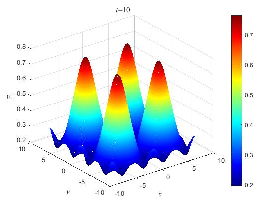
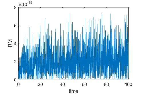
We set the computational domain $\Omega=[-8,8)\times[-8,8)$ . Since the exact solution is not known, we take the numerical solution obtained by the proposed SPRK-3 with the Fourier node $256\times 256$ and the time step $\tau=10^{-3}$ as the “reference solution”. Tables 4 and 5 list the temporal errors of SPRK-2 and SPRK-3 at $T=1$ under different time steps $\tau$ and $\varepsilon$ , where the Fourier node is chosen as $256\times 256$ . It can be clearly observed that SPRK-2 and SPRK-3 are really fourth order accurate and sixth order accurate in time, respectively. Subsequently, the plots for $|E|$ and $N$ at $T=10$ are shown in Figure 5, which implies the numerical solutions obtained by the proposed method are stable in a long time-integration. In Figures 6 and 7, we display the relative residuals on the mass and energy in time interval $[0,200]$ obtained by SPRK-2 and SPRK-3 with the parameter $\varepsilon=\frac{1}{2^{7}}$ , the Fourier node $256\times 256$ and the time step $\tau=1/20$ , which implies that the proposed schemes can preserve the mass and Hamiltonian energy of the QZS (1.1) exactly.

To verify the efficiency of the proposed schemes, we also investigated the maximum norm errors and the CPU time using SPRK-2, SPRK-3 and CNS [8] at $T=1$ with the parameter $\varepsilon=1/2^{3}$ and the Fourier node $256\times 256$ , respectively. The results are summarized in Table 6. As illustrated in the Table, we can draw that for a given global error, the proposed schemes spend much less CPU time than CNS, which implies that our schemes are much more efficient. We note that the “reference solution” is obtained using the proposed SPRK-3 with the parameter $\varepsilon=1/2^{3}$ , the Fourier node $256\times 256$ and the time step $\tau=10^{-3}$ , respectively.

Subsequently, by taking the initial conditions (5.3), the Fourier node $256\times 256$ and the time step $\tau=1/100$ , we apply SPRK-2 and SPRK-3 to study the convergence rates of the QZS (1.1) to its limiting model, i.e. the classical ZS ( $\varepsilon=0$ ), respectively. Figure 8 shows the maximum norm errors calculated by using SPRK-2 and SPRK-3 between the QZS (1.1) and the corresponding classical ZS at $T=10$ with different parameters $\varepsilon=2^{-(2j+1)},j=2,3,4,5,6,7$ . As illustrated in the figures, the solution of the QZS (1.1) with the initial conditions (5.3) converges to the classical ZS quadratically with respect to $\varepsilon$ , which is consistent with the existing theoretical result presented in [16].

Table 4: Temporal errors provided by SPRK-2 at

T=1

for the QZS (1.1) with (5.3) and different

\varepsilon

$e_{\varepsilon}(1)$	$\tau_{0}=1/4$	$\tau_{0}/2$	$\tau_{0}/2^{2}$	$\tau_{0}/2^{3}$	$\tau_{0}/2^{4}$
$\varepsilon=\frac{1}{2^{2}}$	7.05e-5	4.99e-6	3.32e-7	2.11e-8	1.32e-9
rate	-	3.82	3.91	3.98	4.00
$\varepsilon=\frac{1}{2^{3}}$	6.03e-5	4.50e-6	2.93e-7	1.85e-8	1.16e-9
rate	-	3.75	3.94	3.99	4.00
$\varepsilon=\frac{1}{2^{4}}$	4.67e-5	3.45e-6	2.24e-7	1.41e-8	8.83e-10
rate	-	3.76	3.95	3.99	4.00
$\varepsilon=\frac{1}{2^{5}}$	4.30e-5	3.16e-6	2.04e-7	1.29e-8	8.07e-10
rate	-	3.77	3.95	3.99	4.00
$\varepsilon=\frac{1}{2^{6}}$	4.20e-5	3.08e-6	2.00e-7	1.26e-8	7.88e-10
rate	-	3.77	3.95	3.99	4.00
$\varepsilon=\frac{1}{2^{7}}$	1.46e-5	3.07e-6	1.98e-7	1.25e-8	7.83e-10
rate	-	3.77	3.95	3.99	4.00
$n_{\varepsilon}(1)$	$\tau_{0}=1/4$	$\tau_{0}/2$	$\tau_{0}/2^{2}$	$\tau_{0}/2^{3}$	$\tau_{0}/2^{4}$
$\varepsilon=\frac{1}{2^{2}}$	2.30e-5	1.51e-6	9.59e-8	6.00e-9	3.75e-10
rate	-	3.92	3.98	4.00	4.00
$\varepsilon=\frac{1}{2^{3}}$	9.79e-6	6.20e-7	3.89e-8	2.43e-9	1.52e-10
rate	-	3.98	4.00	4.00	4.00
$\varepsilon=\frac{1}{2^{4}}$	9.33e-6	6.00e-07	3.79e-8	2.37e-9	1.49e-10
rate	-	3.96	3.99	4.00	4.00
$\varepsilon=\frac{1}{2^{5}}$	1.01e-5	6.57e-7	4.15e-8	2.60e-9	1.63e-10
rate	-	3.95	3.98	4.00	4.00
$\varepsilon=\frac{1}{2^{6}}$	1.03e-5	6.71e-7	4.24e-8	2.66e-9	1.66e-10
rate	-	3.95	3.98	4.00	4.00
$\varepsilon=\frac{1}{2^{7}}$	1.04e-5	6.74e-7	4.27e-8	2.68e-9	1.67e-10
rate	-	3.95	3.98	4.00	4.00

Table 5: Temporal errors provided by SPRK-3 at

T=1

for the QZS (1.1) with (5.3) and different

\varepsilon

$e_{\varepsilon}(1)$	$\tau_{0}=1/4$	$\tau_{0}/2$	$\tau_{0}/2^{2}$	$\tau_{0}/2^{3}$
$\varepsilon=\frac{1}{2^{2}}$	2.95e-6	6.41e-8	1.10e-9	1.76e-11
rate	-	5.53	5.87	5.97
$\varepsilon=\frac{1}{2^{3}}$	1.63e-6	2.95e-8	4.78e-10	7.54e-12
rate	-	5.79	5.95	5.99
$\varepsilon=\frac{1}{2^{4}}$	1.19e-6	2.13e-8	3.44e-10	5.42e-12
rate	-	5.80	5.95	5.99
$\varepsilon=\frac{1}{2^{5}}$	1.08e-6	1.91e-8	3.08e-10	4.86e-12
rate	-	5.82	5.95	5.99
$\varepsilon=\frac{1}{2^{6}}$	1.05e-6	1.86e-8	3.00e-10	4.72e-12
rate	-	5.82	5.96	5.99
$\varepsilon=\frac{1}{2^{7}}$	1.04e-6	1.85e-8	2.98e-10	4.69e-12
rate	-	5.82	5.96	5.99
$n_{\varepsilon}(1)$	$\tau_{0}=1/4$	$\tau_{0}/2$	$\tau_{0}/2^{2}$	$\tau_{0}/2^{3}$
$\varepsilon=\frac{1}{2^{2}}$	2.70e-7	5.10e-9	8.41e-11	1.33e-12
rate	-	5.73	5.92	5.98
$\varepsilon=\frac{1}{2^{3}}$	6.89e-8	1.18e-9	1.89e-11	3.01e-13
rate	-	5.86	5.96	5.99
$\varepsilon=\frac{1}{2^{4}}$	1.24e-7	2.08e-9	3.31e-11	5.33e-13
rate	-	5.90	5.97	5.98
$\varepsilon=\frac{1}{2^{5}}$	1.56e-7	2.60e-9	4.14e-11	6.91e-13
rate	-	5.90	5.97	5.99
$\varepsilon=\frac{1}{2^{6}}$	1.63e-7	2.72e-9	4.32e-11	8.00e-13
rate	-	5.90	5.98	5.98
$\varepsilon=\frac{1}{2^{7}}$	1.65e-7	2.75e-9	4.37e-11	7.29e-13
rate	-	5.90	5.98	5.98

Table 6: Numerical errors and computational CPU times using three numerical schemes solving the QZS (1.1) with the initial conditions (5.3) at

T=1

, the parameter

\varepsilon=1/2^{3}

and the Fourier node

256\times 256

Scheme	$\tau$	$e_{\varepsilon}(1)$	$n_{\varepsilon}(1)$	CPU time (s)
CNS [8]	$1.0\times 10^{-5}$	7.18e-10	1.22e-09	224.19
SPRK-2	$1.0\times 10^{-2}$	1.94e-10	2.55e-11	5.27
SPRK-3	$5.0\times 10^{-2}$	1.26e-10	4.99e-12	2.68

5.2 Dynamic simulation of one dimensional QZS

Example 5.3. In this subsection, we choose the initial conditions as (cf. [58, 59])

\begin{split}&E_{0}(x)={\rm i}\sum\limits_{j=1}^{2}\sqrt{2\left(1-V_{j}^{2}\right)}\operatorname{sech}\left(x-x_{j}\right)e^{{\rm i}V_{j}\left(x-x_{j}\right)/2},\\ &N_{0}(x)=-2\sum\limits_{j=1}^{2}\operatorname{sech}^{2}\left(x-x_{j}\right),\\ &N_{1}(x)=-4\sum\limits_{j=1}^{2}V_{j}\operatorname{sech}^{2}\left(x-x_{j}\right)\operatorname{tanh}\left(x-x_{j}\right),\ x\in\Omega,\end{split}

(5.4)

where $x_{1}$ and $x_{2}$ are initial locations of the two solitary waves, and $V_{1}$ and $V_{2}$ are the propagation velocity and the sign means moving to the right or left. For brevity, all computations are performed by using SPRK-2 with the Fourier node 4000 and the time step $\tau=1/20$ , where the computational domain is chosen as $\Omega=[-200,200)$ . Moreover, we take the following parameters as:

•

Case I: $x_{1}=-x_{2}=-30,\ V_{1}=-V_{2}=\frac{1}{2}$ ;
•

Case II: $x_{1}=-x_{2}=-30,\ V_{1}=\frac{3}{4},\ V_{2}=-\frac{1}{2}$ ;
•

Case III: $x_{1}=-x_{2}=-5,\ V_{1}=\frac{3}{4},\ V_{2}=-\frac{1}{2}$ .

The surface plots of the interaction of two solitary waves for QZS ( $\varepsilon\neq 0$ ) (1.1) and the classical ZS ( $\varepsilon=0$ ) under cases (I)-(III) are demonstrated in Figures 9-11, respectively, which implies that: (i) all the collisions between two solitons are not elastic; (ii) when two initially well-separated solitons with opposite propagation velocities (cf. case (I) in Figure 9) or different propagation speeds (cf. case (II) in Figure 10), they collide and fuse into a new soliton with the strengthened amplitude and the narrower width; (iii) the amplitude-weakened solitons with propagation speeds changed and some small radiation are generated during the collision; (iv) when the initial locations are not initially well-separated (cf. case (III) in Figure 11), the dynamics is considerably more complicated, it seems that a periodic perturbation on the position of some localized pulse. In addition, from Figures 9-11, we also observe that the soliton-soliton collisions of the QZS are more unstable than the corresponding classical ZS after collision, and the quantum effect makes the chaos much more obvious. The larger the quantum effect is, the more obvious the spatiotemporal chaos is. In particular, for the strong quantum regime $\varepsilon=1$ , there are small outgoing waves emitting before colliding, and the chaos is much more obvious than the classical one. In Figures 12 and 13 , we display the relative residuals on mass and energy provided by SPRK-2, which shows that the proposed scheme can conserve the discrete mass and energy exactly.

Example 5.4. The initial conditions are chosen as (cf. [41])

\begin{split}&E_{0}(x)=E_{0}(1+\beta\cos(kx)),\\ &N_{0}(x)=-\sqrt{2}E_{0}k\beta\cos(kx),\quad N_{1}(x)=0,\end{split}

(5.5)

where $E_{0}=(k/\sqrt{2})(1+\varepsilon^{2}k^{2})$ is the amplitude of the pump Langmuir wave, $0<k<\sqrt{2}E_{0}$ and $\beta$ represents a relatively small constant to emphasize that the perturbation is small.

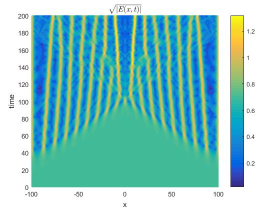
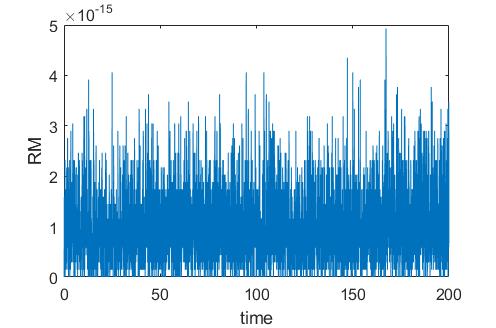
We take the computational domain $\Omega=[-100,100)$ and set the parameters as $k=0.7$ , $\beta=0.001$ . For brevity, all computations are performed by using SPRK-2 over the time interval $[0,200]$ with the Fourier node 2000 and the time step $\tau=1/20$ . Figure 14 shows that many solitary patterns can be generated and excited through the modulational instability of unstable harmonic modes. It can be clearly observed that the QZS (1.1) is more unstable than the corresponding classical ZS. In particular, for the strong quantum regime $\varepsilon=1$ , numerical simulation also indicates that the motion of the trains leads to more collision among the neighboring coherent solitary patterns, and fuse into the newer pattern with strengthened amplitude. This space-time evolution reveals that the spatiotemporal chaos is more obvious as the classical one. The numerical results are in good agreement with the results given in [41]. Figure 15 display the relative residuals on the mass and energy provided by SPRK-2 with the parameter $\varepsilon=0$ , which implies that SPRK-2 preserve the mass and energy conservations exactly.

6 Conclusions

In this paper, we develop a novel class of high-order accurate structure-preserving methods for solving the QZS (1.1), which is based on the idea of the QAV approach, the symplectic RK method together with the standard Fourier pseudo-spectral method in space. We show that the proposed scheme can preserve the discrete mass and original Hamiltonian energy exactly. In addition, an efficient fixed point iteration is presented to solve the resulting nonlinear equations of the proposed scheme. Numerical experiments for the QZS (1.1) are carried out to illustrate the capability and accuracy of the new schemes. We also use our new scheme to numerically simulate the soliton-soliton interaction and the pattern dynamics of the QZS (1.1) in 1D. We numerically observe that the numerical solution of the QZS (1.1) converges to the classical Zakharov system quadratically in the semi-classical limit. As far as we know, there are some works (e.g., see Refs. [8, 59]) on optimal error estimates of second-order mass- and energy-conserving schemes for the QZS (1.1), but the error estimate of high-order ones is still not available. Thus, how to establish optimal error estimates for the proposed methods will be an interesting topic for future studies.

Acknowledgments

The work is supported by the National Natural Science Foundation of China (Grant Nos. 12261097, 12261103), and the Yunnan Fundamental Research Projects (Grant Nos. 202101AT070208, 202301AT070117, 202101AS070044) and Innovation team of School of Mathematics and Statistics, Yunnan University (No. ST20210104). The first author is in particular grateful to Prof. Weizhu Bao for fruitful discussions.

Conflict of interest

The authors declare that they have no conflict of interest.

References

[1] W. Bao and C. Su. Uniform error bounds of a finite difference method for the Zakharov system in the subsonic limit regime via an asymptotic consistent formulation. Multiscale Model. Simul., 15:977–1002, 2017.
[2] W. Bao and C. Su. A uniformly and optically accurate method for the Zakharov system in the subsonic limit regime. SIAM J. Sci. Comput., 40:A929–A953, 2018.
[3] W. Bao and F. Sun. Efficient and stable numerical methods for the generalized and vector Zakharov system. SIAM J. Sci. Comput., 26:1057–1088, 2005.
[4] L. Barletti, L. Brugnano, G. F. Caccia, and F. Iavernaro. Energy-conserving methods for the nonlinear Schrödinger equation. Appl. Math. Comput., 318:3–18, 2018.
[5] S. Baumstark and K. Schratz. Asymptotic preserving trigonometric integrators for the quantum Zakharov system. BIT, 61:61–81, 2021.
[6] L. Brugnano and F. Iavernaro. Line Integral Methods for Conservative Problems. Chapman et Hall/CRC: Boca Raton, FL, USA, 2016.
[7] L. Brugnano, F. Iavernaro, and D. Trigiante. Hamiltonian boundary value methods (energy preserving discrete line integral methods). J. Numer. Anal. Ind. Appl. Math., 5:17–37, 2010.
[8] Y. Cai, J. Fu, J. Liu, and T. Wang. A fourth-order compact finite difference scheme for the quantum Zakharov system that perfectly inherits both mass and energy conservation. Appl. Numer. Math., 178:1–24, 2022.
[9] Y. Cai and Y. Yuan. Uniform error estimates of the conservative finite difference method for the Zakharov system in the subsonic limit regime. Math. Comp., 87:1191–1225, 2018.
[10] J. Chen and M. Qin. Multi-symplectic Fourier pseudospectral method for the nonlinear Schrödinger equation. Electron. Trans. Numer. Anal., 12:193–204, 2001.
[11] Y. Chen, Y. Gong, Q. Hong, and C. Wang. A novel class of energy-preserving Runge-Kutta methods for the Korteweg-de Vries equation. Math. Theor. Meth. Appl., 15:768–792, 2022.
[12] D. Cohen and E. Hairer. Linear energy-preserving integrators for Poisson systems. BIT, 51:91–101, 2011.
[13] J. Cui, Y. Wang, and C. Jiang. Arbitrarily high-order structure-preserving schemes for the Gross-Pitaevskii equation with angular momentum rotation. Comput. Phys. Commun., 261:107767, 2021.
[14] A. S. Davydov. Solitons in molecular systems. Phys. Scr., 20:387–394, 1979.
[15] L. M. Degtyarev, V. G. Nakhankov, and L. I. Rudakov. Dynamics of the formation and interaction of langmuir solitons and strong turbulence. Sov. Phys. JETP, 40:264–268, 1974.
[16] Y. Fang, H. Kuo, H. Shih, and K. Wang. Semi-classical limit for the quantum Zakharov system. Taiwan. J. Math., 23:925–949, 2019.
[17] Y. Fang, C. Lin, and J. Segata. The fourth-order nonlinear Schrödinger limit for quantum Zakharov system. Z. Angew. Math. Phys., 67:145, 2016.
[18] Y. Fang and K. Nakanishi. Global well-posedness and scattering for the quantum Zakharov system in $L^{2}$ . Proc. Amer. Math. Soc., 6:21–32, 2019.
[19] Y. Fu, W. Cai, and Y. Wang. A linearly implicit structure-preserving scheme for the fractional sine-Gordon equation based on the IEQ approach. Appl. Numer. Math., 160:368–385, 2021.
[20] L. G. Garcia, F. Haas, L. P. L. de Oliveira, and J. Goedert. Modified Zakharov equations for plasmas with a quantum correction. Phys. Plasmas, 12:012302, 2005.
[21] L. Glangetas and F. Merle. Existence of self-similar blow-up solutions for Zakharov equation in dimension two. Part I. Comm. Math. Phys., 160:173–215, 1994.
[22] R. T. Glassey. Convergence of an energy-preserving scheme for the Zakharov equations in one space dimension. Math. Comp., 58:83–102, 1992.
[23] Y. Gong, Q. Hong, C. Wang, and Y. Wang. Quadratic auxiliary variable Runge-Kutta methods for the Camassa-Holm equation. Adv. Appl. Math. Mech. (accepted), 2022.
[24] Y. Gong, J. Zhao, and Q. Wang. Arbitrarily high-order unconditionally energy stable schemes for thermodynamically consistent gradient flow models. SIAM J. Sci, Comput., 42:B135–B156, 2020.
[25] B. Guo, Z. Gan, L. Kong, and J. Zhang. The Zakharov System and its Soliton Solutions. Science Press, New York, 2016.
[26] F. Haas. Quantum Plasmas. Quantum Plasmas: An Hydrodynamic Approach, Springer Series on Atomic, Optical, and Plasma Physics, Springer New York, 2011.
[27] F. Haas and P. K. Shukla. Quantum and classical dynamics of Langmuir wave packets. Phys. Rev. E, 79:066402, 2009.
[28] E. Hairer. Energy-preserving variant of collocation methods. J. Numer. Anal. Ind. Appl. Math., 5:73–84, 2010.
[29] E. Hairer, C. Lubich, and G. Wanner. Geometric Numerical Integration: Structure-Preserving Algorithms for Ordinary Differential Equations. Springer-Verlag, Berlin, 2nd edition, 2006.
[30] C. Jiang, W. Cai, and Y. Wang. A linearly implicit and local energy-preserving scheme for the sine-Gordon equation based on the invariant energy quadratization approach. J. Sci. Comput., 80:1629–1655, 2019.
[31] C. Jiang, J. Cui, X. Qian, and S. Song. High-order linearly implicit structure-preserving exponential integrators for the nonlinear Schrödinger equation. J. Sci. Comput., 90:1–27, 2022.
[32] C. Jiang, Y. Wang, and Y. Gong. Arbitrarily high-order energy-preserving schemes for the Camassa-Holm equation. Appl. Numer. Math., 151:85–97, 2020.
[33] S. Jin, P. A. Markowich, and C. Zheng. Numerical simulation of a generalized Zakharov system. J. Comput. Phys., 201:376–395, 2004.
[34] S. Jin and C. Zheng. A time-splitting spectral method for the generalized Zakharov system in multi-dimensions. J. Sci. Comput., 26:127–149, 2006.
[35] H. Li, Y. Wang, and M. Qin. A sixth order averaged vector field method. J. Comput. Math., 34:479–498, 2016.
[36] Y. Li and X. Wu. General local energy-preserving integrators for solving multi-symplectic Hamiltonian PDEs. J. Comput. Phys., 301:141–166, 2015.
[37] Y. Li and X. Wu. Functionally fitted energy-preserving methods for solving oscillatory nonlinear Hamiltonian systems. SIAM J. Numer. Anal., 54:2036–2059, 2016.
[38] M. Marklund. Classical and quantum kinetics of the Zakharov system. Phys. Plasmas, 12:082110, 2005.
[39] V. Masselin. A result of the blow-up rate for the Zakharov system in dimension 3. SIAM J. Math. Anal., 33:440–447, 2001.
[40] L. Mei, L. Huang, and X. Wu. Energy-preserving exponential integrators of arbitrarily high order for conservative or dissipative systems with highly oscillatory solutions. J. Comput. Phys., 442:110429, 2021.
[41] A. P. Misra and P. K. Shukla. Pattern dynamics and spatiotemporal chaos in the quantum Zakharov equations. Phys. Rev. E, 97:056401, 2009.
[42] Y. Miyatake and J. C. Butcher. A characterization of energy-preserving methods and the construction of parallel integrators for Hamiltonian systems. SIAM J. Numer. Anal., 54:1993–2013, 2016.
[43] G. R. W. Quispel and D. I. McLaren. A new class of energy-preserving numerical integration methods. J. Phys. A: Math. Theor., 41:045206, 2008.
[44] J. M. Sanz-Serna. Runge-Kutta schemes for Hamiltonian systems. BIT, 28:877–883, 1988.
[45] J. M. Sanz-Serna and J. G. Verwer. Conservative and nonconservative schemes for the solution of the nonlinear Schrödinger equation. IMA J. Numer. Anal., 6:25–42, 1986.
[46] J. Shen and T. Tang. Spectral and High-Order Methods with Applications. Science Press, Beijing, 2006.
[47] J. Shen, J. Xu, and J. Yang. The scalar auxiliary variable (SAV) approach for gradient. J. Comput. Phys., 353:407–416, 2018.
[48] J. Shen, J. Xu, and J. Yang. A new class of efficient and robust energy stable schemes for gradient flows. SIAM Rev., 61:474–506, 2019.
[49] J. Shen and N. Zheng. Efficient and accurate SAV schemes for the generalized Zakharov systems. Discrete Contin. Dyn. Syst. Ser. B, 26:645–666, 2021.
[50] W. Tang and Y. Sun. Time finite element methods: a unified framework for numerical discretizations of ODEs. Appl. Math. Comput., 219:2158–2179, 2012.
[51] B. K. Tapley. Geometric integration of ODEs using multiple Quadratic Auxiliary Variables. SIAM. J. Sci. Comput., 44:A2651–A2668, 2022.
[52] B. Wang and X. Wu. Functionally-fitted energy-preserving integrators for Poisson systems. J. Comput. Phys., 364:137–152, 2018.
[53] Y. Xia, Y. Xu, and C. Shu. Local discontinuous Galerkin methods for the generalized Zakharov system. J. Comput. Phys., 229:1238–1259, 2010.
[54] A. Xiao, C. Wang, and J. Wang. Conservative linearly-implicit difference scheme for a class of modified Zakharov systems with high-order space fractional quantum correction. Appl. Numer. Math., 146:379–399, 2019.
[55] X. Yang, J. Zhao, and Q. Wang. Numerical approximations for the molecular beam epitaxial growth model based on the invariant energy quadratization method. J. Comput. Phys., 333:104–127, 2017.
[56] V. E. Zakharov. Collapse of langmuir waves. Sov. Phys. JETP, 35:908–914, 1972.
[57] F. Zhang, V. M. Pérez-García, and L. Vázquez. Numerical simulation of nonlinear Schröinger systems: a new conservative scheme. Appl. Math. Comput., 71:165–177, 1995.
[58] G. Zhang. Time splitting combined with exponential wave integrator fourier pseudospectral method for quantum Zakharov system. Discrete Contin. Dyn. Syst. Ser. B, 27:2587–2606, 2022.
[59] G. Zhang and C. Su. A conservative linearly-implicit compact difference scheme for quantum Zakharov system. J. Sci. Comput., 87:71, 2021.