Applying Opponent Modeling for Automatic Bidding in Online Repeated Auctions

The main results of auction theory have been consolidated in McAfee and McMillan (1987). In addition, Mittelmann et al. (2022) discussed the representation and reasoning processes associated with auctions. For prior-independent mechanisms, such as fisrt-price and second-price auctions, the seller’s revenue is the same when the bidders respond optimally Myerson (1981). This has inspired research on prior-dependent auctions with IC constraint, where the truthful bidding strategy is the dominant strategy for bidders.

The well-known revenue-maximizing mechanism is the Myerson auction Myerson (1981), which is the optimal mechanism that satisfies the IC constraint under the premise that the value of the bidders is public information. In the Myerson auction, each bidder’s value $v_{i}$ is transformed into a virtual value $w_{i}=g_{i}(v_{i})$, after which a second-price auction with a reserve price of 0 is conducted using the set of virtual values $\@vec{w}$. The virtual value function $g_{i}$ is determined by the distribution $F_{i}$ and the density function $f_{i}$ associated with $v_{i}$.

In fact, the virtual value function $g_{i}$ plays a key role in determining both the allocation and payment of the mechanism.

At this point, it is assumed that the joint value distribution of the other bidders is represented as $F_{-i}$. Consequently, the utility of the bidder $i$ can be expressed as:

Here, $dv_{-i}=dv_{1}dv_{2}\cdots dv_{i-1}dv_{i+1}\cdots dv_{n}$ and $b_{i}=B_{i}(v_{i})$. In the context of single-item auctions, it is necessary for the allocation to be 0 or 1. As a result, the above equation can be reformulated as:

Here, $\mathbb{I}$ denotes the indicator function, and $a_{i}=a_{i}(b_{i},B_{-i}(v_{-i}))$. The seller’s revenue can be defined as:

The Myerson mechanism has been proven to satisfy the IC constraint, indicating that the truthful bidding strategy $B_{i}(v_{i})=v_{i}$ is the optimal response to the Myerson mechanism Myerson (1981).

We consider the standard setting as an example. There are two bidders and their value distribution is identical, represented as $v_{i}\sim U[0,1]$. If the seller employs the Myerson mechanism, the virtual value function is $g_{i}(v_{i})=2v_{i}-1$. In response, both bidders choose to adopt the truthful bidding strategy as their best response to the Myerson mechanism. The expected utility of each bidder is $\frac{1}{12}$ and the expected revenue of the seller is $\frac{5}{12}$. However, if the seller adopts the first-price or second-price auction instead, the revenue generated is only $\frac{1}{3}$.

In this paper, online auction means the auctions held in online marketplaces, such as bidding searches on advertising platforms Carrion et al. (2023). In this context, bidders frequently participate in multiple auctions for identical or similar items. This circumstance presents opportunities to implement prior-dependent mechanisms, even when access to the value distribution of bidders is limited. The seller can establish a mechanism that adheres to the IC constraints, requiring bidders to employ a truthful bidding strategy. By collecting bid samples from repeated auctions, the seller can estimate the value distribution of the bidders, denoted as $\@vec{F}$, and subsequently adjust the mechanism parameters to converge towards the optimal Myerson auction.

Myerson Net Duetting et al. (2019) presents a technique that leverages a monotonely increasing parameterized neural network $G$ to acquire virtual value functions $\@vec{g}$ and derive optimal auction mechanisms.

From the definition we can obtain the following property. {theorem} Myerson Net satisfies the IC constraints in single-item auctions. For a Myerson Net $M$, we add a strictly increasing function $Q$ to each virtual value function $G^{\prime}_{i}=Q\circ G_{i}$ that satisfies $G_{i}(b_{i})=0\iff Q\circ G_{i}(b_{i})=0$ to obtain another mechanism $M^{\prime}$. Then $M^{\prime}$ and $M$ have the same allocation and payment rule.

The proof of Theorem 2.1 is given in the supplementary metarial. We use $\cong$ to represent the two different networks with the same allocation and payment mechanism. Since the Myerson Net satisfies the IC constraints, we can assume that the bidders will adopt the truthful bidding strategy. Using the real bids obtained in repeated auctions, the seller updates the network parameter $\theta$ with the objective of maximizing revenue $r$, which results in the convergence of the virtual value function $G$ to the optimal function $\@vec{g}$ corresponding to the true value distribution of the bidders. This suggests that the system converges to the revenue-maximizing Myerson mechanism when bidders bid truthfully in this environment.

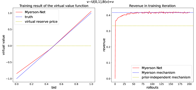
Figure 1 provides an example of the application in the standard setting. The figure on the left shows that the seller has learned the optimal virtual value function in 200 iterations. The figure on the right shows the change in revenue in the learning iterations. We can see that the seller using Myerson Net obtains optimal revenue, which exceeds the prior-independent mechanism.

Myerson Net provides an approach as a revenue-maximizing mechanism for online repeated auctions. Since Myerson Net satisfies the incentive compatibility constraint, the optimal strategy for bidders in a single auction round is the truthful bidding strategy. However, some previous studies have found that bidders in repeated auctions have more efficient strategies, which requires them to bid according to some specific distribution instead of true value distribution. Although bidders initially lose some utility under the IC-constrained mechanism, untruthful bids can lead the seller to misestimate the value distribution and increase bidders’ long-term utility.

Tang’s research Tang and Zeng (2018) defines the induced game of auction when the seller adjusts the mechanism according to the bids. As an example, the Myerson mechanism induces a game in which the players contain only bidders. In this game, bidders adopt specific bidding strategies rather than the truthful strategy, and their utility is derived from the Myerson mechanism that runs based on bids.

We present the partial payment matrix for the induced game of the single-item, two-bidder auction in the supplementary material and we have the following property. {theorem} We assume that there are two bidders and their value distribution is $U[0,1]$ (standard setting), the induced game is as detailed in Definition 2. For strategic bidders with a limited strategy space $B(v)=\alpha v$ (referred to as the linear shading strategy space), the Nash equilibrium of the induced game yields $B_{i}(v_{i})=\frac{5}{14}v_{i}$. However, in cases where bidders have access to arbitrary monotone increasing strategies, a Nash equilibrium emerges with bidding strategies represented as $B_{i}(v_{i})=\frac{v_{i}+1}{4}$. For the two bidders in the standard setting, the expected utility in each round of the auction when they employ a truthful bidding strategy is $\frac{1}{12}$. When their bidding strategy is $B_{i}(v_{i})=\frac{v_{i}+1}{4}$, the expected utility is $\frac{1}{6}$. This suggests that strategic bidders can increase utility through specific bidding strategies in the induced game. The proof of Theorem 2.2 is given in the supplementary material.

From Theorem 2.2 we can see that bidders learn different equilibria when their strategy space is limited. Since an optimal mechanism can be learned through strategy networks, we consider setting up a similar structure for the strategy learning of bidders.

If we consider static strategies, then for the game induced by the Myerson auction, the Nash equilibrium in the standard setting is:

However, its drawback is that $B(v)\leq v$ does not always hold. This equilibrium strategy may lead to negative utilities for bidders with $v<\frac{1}{3}$. When bidders do not have access to the dynamic mechanism update method, adopting a bidding strategy that does not satisfy IR (individual rationality) may reduce the bidders’ expected utility. Therefore, we require that the bidding strategy obtained by the network satisfies the following requirements:

• 1)

  $B(v)$ is increasing function about $v$,

• 2)

  $v\geq B(v)\geq 0$.

We propose a parametric network (Bid Net) to represent the bidder’s strategy. The network first inputs the received values $v_{i}$ from the distribution $F_{i}$ into a multilayer perceptron. Monotonic outputs $b_{i}^{*}=B_{i}^{*}(v_{i})$ are combined with regularization constraints $B_{i}(v_{i})=\text{Min}[B_{i}^{*}(v_{i}),v_{i}]$. This ensures that the output of the network meets both of these requirements. Since Bid Net training requires the use of a gradient propagation algorithm and the operators associated with sorting $(Min,Max,Sort)$ cannot propagate the gradient, we use NeuralSort Grover et al. (2019); Liu et al. (2021) as an approximation in our network. The structure of the Bid Net is shown in Figure 2.

We assume that bidders and the seller interact in an infinitely repeated auction with identical items and update their strategies after each auction round. At the moment $t$, the seller first announces the current parameter $\theta$ of the mechanism. The strategy of the bidders $\@vec{\pi}$ and the seller $\theta$ determines the utility $u^{t}_{i}=a^{t}_{i}v^{t}_{i}-p^{t}_{i}$ and the revenue $r^{t}$ of this auction round. For strategic bidders and the seller, the observations they receive are the joint bidding $\@vec{b}$, mechanism parameter $\theta$, and their rewards ($u^{t}_{i}$ or $r^{t}$). When the value distribution is constant, the joint bidding distribution $\@vec{b}$ is directly determined by the joint strategy $\@vec{\pi}$. Therefore, we use strategies $\@vec{\pi}$ instead of bids $\@vec{b}$ to represent the action of the bidders in repeated auctions.

Based on the observations and the reward maximization objectives, the agents will update their strategy for the next auction round. We usually assume that the strategic bidder adjusts the previous strategy based on observation:

This forms an MARL system when both the seller and bidders update their strategies through learning. The convergence of the strategy in repeated auctions is consistent with the equilibrium of the induced game, where the bidding strategy and mechanism reach a stable point. Our goal is to provide a learning algorithm for bidders that maximizes their utility as the system converges. When the bidder $i$ is a naive learner Foerster et al. (2018), it will maximize its utility assuming that the other agent strategies remain unchanged:

We can design gradient-based methods with learning rate $\gamma$:

While the naive learner can only engage in inefficient learning process, the opponent modeling approach is able to improve the reward of agents by predicting the change in the opponent’s strategy and selecting the corresponding best response:

A simple assumption in Foerster et al. (2018) is that the other agents are naive learners with lookahead rate $\gamma^{\prime}$, which means that:

In the following sections, we will specifically discuss the design of the opponent modeling algorithm applicable to repeated auctions and propose our strategy learning method in this MARL system.

In this section, we introduce the automatic bidding method for the MARL system in Section 3.2. Since the seller and other bidders also update their strategies, agents must consider both the current utility and the impact on subsequent states when evaluating the strategy $\pi_{i}$. We adopt representation similar to RL (reinforcement learning) and use $Q_{i}$ to denote the utility expectation of the strategy for the bidder $i$, then we have the following:

where $\lambda$ is the discount factor.

For the agent $i$ who needs to choose a strategy at moment $t$, the information available is historical observations before moment $t$. Therefore, it is difficult to obtain unbiased estimates of $Q_{i}$. A direct approximation is $\hat{Q}_{i}=U_{i}(\pi^{t}_{i},\pi^{t}_{-i},\theta^{t})$, which means that the bidder assumes that the subsequent strategy of other agents ($\pi^{t+1}_{-i},\theta^{t+1}$) is not relevant to its strategy $\pi^{t}_{i}$. Then its choice of action at the next moment will be based on the prediction of the opponent’s action:

For the naive learner, it will assume that the strategies of other agents remain unchanged:

Then its gradient update direction for the strategy will be:

More accurate estimations for $U_{i}(\pi^{t}_{i},\pi^{t}_{-i},\theta^{t})$ usually require first-order approximations:

We can obtain different predictions for $(\Delta\hat{\pi}_{-i},\Delta\hat{\theta})$ with opponent modeling methods. The LOLA Foerster et al. (2018) algorithm assumes that the opponent is a naive learner, which means $\Delta\hat{\theta}=\eta\cdot\nabla_{\theta}R(\@vec{\pi},\theta)$. Assuming that the opponent is a LOLA learner leads to high-order LOLA (HOLA). Similar opponent modeling algorithms include SOS (stable opponent shaping) Letcher et al. (2019), COLA (consistent learning with opponent learning awareness) Willi et al. (2022), and others, which effectively learn equilibrium with higher rewards in different game environments.

COLA Willi et al. (2022) points out that the effectiveness of opponent modeling algorithms depends on the consistency of the lookahead rate of all agents. This means that agents need to choose strategy-update approaches with consistency to ensure the convergence of the system. However, we have discussed earlier the asymmetry of the repeated auction environment: bidders have private information (value function) that allows them to adopt specific strategies to improve utility. Training strategies directly using opponent modeling algorithms does not maximize the utility of bidders.

Figure 3 shows the direction of propagation of the network parameter gradient for bidders and the seller in the MARL environment of repeated auctions. We illustrate the necessity of computing the indirect gradient represented by the blue dashed line in the figure in repeated auctions by proving the following property. {theorem} If all bidders use only the gradient which comes directly from the utility to update the strategy under the Myerson Net of the seller, their gradient-based strategy updating will converge to the truthful bidding strategy $B_{i}(v_{i})=v_{i}$. The stable state of the system is where all bidders bidding truthfully.

The proof of Theorem 3.1 is given in the supplementary material. This Theorem indicates that the strategy network of bidder must be trained with the indirect gradient, which requires predicting the impact of bidding strategies on mechanism changes. In order to obtain a more accurate prediction of the $Q_{i}$ function for bidders, we estimate $\mathop{\text{max}}\limits_{\pi_{i}}Q_{i}(\pi_{i},\pi^{t+1}_{-i},\theta^{t+1})$ by modeling $\Delta\hat{\pi}^{t+1}_{-i},\Delta\hat{\theta}^{t+1}$ as functions of $\pi^{t}_{i}$:

Then we have:

The convergence of the system in the repeated auction is equivalent to the convergence of the strategies of each agent. We can simplify the above equation by assuming that $\pi^{t}_{i}=\pi^{t+1}_{i}=\cdots$ and then it will become:

where $\Delta^{k}\hat{\pi}_{-i}(\pi^{t}_{i})$ means the prediction of $\pi_{-i}$ after $k$ updates.

We use $\hat{\pi}_{-i}(\pi^{t}_{i}),\hat{\theta}(\pi^{t}_{i})$ to represent the strategy of other agents when the system converges, which means that:

We can always require that the system converge in finite time by periodic reducing the step size of the strategy updating. Assuming that the system converges after $T$ updates, we have:

When $\lambda\rightarrow 1$, the second item will be sufficiently larger than the first. Then we have:

Thus, the strategy selection function of the agent is as follows:

When a single bidder’s strategy is fixed in a repeated auction, the strategy updates of other bidders and the seller are synchronized and will affect each other. The convergence result is determined by the algorithm used by these agents. To avoid discussing the possibility of different stable points in the system, we assume that the strategy updates of other agents are independent and the bidders’ strategies change slowly $\Delta\hat{\pi}_{-i}(\pi^{t}_{i})\approx 0$. We found this assumption to be valid in our experiments, for predicting the strategies of other agents under the condition that their private information is unknown will lead to a large bias.

We refer to this process (calculating $\hat{\pi}_{-i}(\pi^{t}_{i}),\hat{\theta}(\pi^{t}_{i})$ using $\pi^{t}_{i}$) as the inner loop part of the algorithm. When the seller adopts Myerson Net as the mechanism, its strategy updating process according to historical bids is similar to a naive learner. We can simulate this process in the inner loop through the Myerson Net by constraining the bidder strategies to $\pi^{t}_{i},\pi^{t-1}_{-i}$. The complete procedure for the inner loop is given in Algorithm 1.

Based on the strategy predictions of the other agents obtained from the inner loop, we can derive the bidding strategy that maximizes the expected utility. To avoid the instability caused by rapid strategy changes, we restrict the step size by $\lvert\Delta\pi_{i}\rvert\leq d$. Then our goal is to solve the optimization problem:

Since the parameters in the optimization objective contain the output of the inner loop, it is difficult to calculate the strategy gradient directly. We give the approximate calculation based on the PG (pseudo-gradient) by defining the pseudo-gradient obtained from $\Delta\pi_{i}$ as:

From the definition we can see that, given the strategy update $\Delta\pi_{i}$, it is possible to calculate the pseudo-gradients with the inner loop. For the algorithm to choose an update step that is close to the direction of the true gradient, we generate a set of different directions of $\Delta\pi_{i}$ and select the positive gradient with the largest absolute value from all pseudo-gradients as the update direction of the Bid Net. The complete procedure for the PG algorithm is given in Algorithm 2. We want the algorithm to converge to the equilibrium of the repeated auction-induced game. For a single-item Myerson auction that induces a game among bidders, we give proof of the convergence in the supplementary material.

Assuming that other bidders use static strategies $\pi_{-i}$, $\hat{\theta}(\Delta\pi_{i})$ obtained from the inner loop belonging to the optimal mechanisms and $K^{\prime}\rightarrow\infty$ in algorithm 2, the strategic bidder using the PG algorithm will converge to the strategy with optimal utility. When all bidders adopt the PG algorithm, the equilibrium of the Myerson auction-induced game is the only stable point of the system.

In our experiments, we find that the result of the algorithm satisfies this theorem even if the inner loop does not converge and $K^{\prime}$ is finite. Our algorithm PG converges to the equilibrium of all the games induced by the auction, even in multiple-bidders settings.

We compare linear shading strategies and Bid Net, which is trained using PG and RL algorithms. Our evaluation takes place in the standard setting, with another bidder consistently employing the truthful bidding strategy. The results are given in Figure 4.

From the figure, we can see that the network trained using RL converges to the truthful bidding strategy. The linear shading strategy trained through PG improves the utility of the strategic bidder, but does not approach the optimal strategy. The strategy produced by Bid Net trained with the PG algorithm closely approximates the optimal strategy. This experiment underscores the efficiency of Bid Net in accurately representing bidding strategies, while linear shading strategies do not contain the optimal strategy. The gap between the seller’s revenue and the theoretical value may arise from the fact that we set a very small reserve price.

We compare the utility of agents with different strategy learning algorithms. The environment is the standard setting, and all bidders employ the linear shading strategy $B_{i}(v_{i})=\alpha_{i}v_{i}$. In this environment, both bidders will adopt the same algorithm to learn the strategy. At the end of each auction round $t$, bidders and the seller will observe the strategies $(\alpha^{t}_{i},\alpha^{t}_{-i},\theta^{t})$ and the corresponding rewards $(u^{t}_{i},u^{t}_{-i},r^{t})$. Subsequently, the seller updates the mechanism in accordance with the Myerson Net, while the bidders adjust their strategies based on their respective learning algorithms. An equilibrium of the above system is $\alpha_{1}=\alpha_{2}=\frac{5}{14}$.

We compare the PG algorithm with opponent modeling and equilibrium solving algorithms (RL, LOLA Foerster et al. (2018), LA Zhang and Lesser (2010b), CO Mescheder et al. (2017), CGD Schaefer and Anandkumar (2019), LSS Mazumdar et al. (2019), SOS Letcher et al. (2019)) in the aforementioned environment. Figure 5 illustrates the evolution of agent strategy parameters during training. The results demonstrate that the majority of algorithms converge towards the truthful bidding strategy, aligning with the conclusion in Theorem 3.1. Algorithms that incorporate opponent predictions improve utility but display a degree of instability. Notably, the PG algorithm’s training results closely approximate the Nash equilibrium strategy. The slight deviation from equilibrium could be attributed to the implementation of a sufficiently small reserve price. The average utility of various agent systems is shown in Figure 6, where the PG algorithm attains the highest average utility in the automated bidding task, consistent with Theorem 3.2.

We conducted a series of experiments within diverse environments and with varying opponent strategies. Experiments in which other bidders use static strategies include: ① Standard setting with a truthful bidding opponent. In this scenario, another bidder consistently employs the truthful bidding strategy. ② Standard setting with a Nash equilibrium opponent. In this setup, another bidder adheres to the Nash equilibrium bidding strategy. ③ Asymmetric value distribution. Here, the private value distribution of bidders exhibits asymmetry. ④ Dynamic value distribution. In this experiment, the value distribution function of the strategic bidder evolves over time. ⑤ Single-item three-bidders auction. This experiment extends to a scenario with more than two bidders.

Experiments involving dynamic strategies employed by other bidders encompass: ⑥ LOLA algorithm opponent. Here, another bidder updates its strategy using the LOLA algorithm. ⑦ SOS algorithm opponent. In this case, another bidder adjusts its strategy using the SOS algorithm. In the two sets of experiments described above, the opponent bidder uses linear shading strategies.

We evaluate the effectiveness of the algorithms to improve the utility of the strategic bidder after 400 iterations. The results are presented in Table 1. The algorithms used for comparison (RL, LOLA, SOS) are experimented with both Bid Net and linear shading strategies, and the results in the table are taken from the better of the two. We see that the Bid Net trained with PG always maximizes the utility of the strategic bidder. More details of the setting and figures of the experiment are given in the supplementary material.

References

- (1)
- Afshar et al. (2021) Reza Refaei Afshar, Jason Rhuggenaath, Yingqian Zhang, and Uzay Kaymak. 2021. A Reward Shaping Approach for Reserve Price Optimization using Deep Reinforcement Learning. In 2021 International Joint Conference on Neural Networks. 1–8.
- Bagnall and Toft (2006) Anthony Bagnall and Iain Toft. 2006. Autonomous adaptive agents for single seller sealed bid auctions. Autonomous Agents and Multi-Agent Systems 12 (2006), 259–292.
- Balcan et al. (2018) Maria-Florina Balcan, Tuomas Sandholm, and Ellen Vitercik. 2018. A General Theory of Sample Complexity for Multi-Item Profit Maximization. In Proceedings of the 2018 ACM Conference on Economics and Computation. 173–174.
- Balcan et al. (2016) Maria-Florina F Balcan, Tuomas Sandholm, and Ellen Vitercik. 2016. Sample Complexity of Automated Mechanism Design. In Advances in Neural Information Processing Systems, Vol. 29.
- Cai et al. (2018) Qingpeng Cai, Aris Filos-Ratsikas, Pingzhong Tang, and Yiwei Zhang. 2018. Reinforcement Mechanism Design for E-Commerce. In Proceedings of the 2018 World Wide Web Conference. 1339–1348.
- Carrion et al. (2023) Carlos Carrion, Zenan Wang, Harikesh Nair, Xianghong Luo, Yulin Lei, Peiqin Gu, Xiliang Lin, Wenlong Chen, Junsheng Jin, Fanan Zhu, et al. 2023. Blending advertising with organic content in e-commerce via virtual bids. In Proceedings of the AAAI Conference on Artificial Intelligence, Vol. 37. 15476–15484.
- Cli (1997) Dave Cli. 1997. Minimal-intelligence agents for bargaining behaviors in market-based environments. Hewlett-Packard Labs Technical Reports (1997).
- Cole and Roughgarden (2014) Richard Cole and Tim Roughgarden. 2014. The Sample Complexity of Revenue Maximization. In Proceedings of the Forty-Sixth Annual ACM Symposium on Theory of Computing. 243–252.
- Duetting et al. (2019) Paul Duetting, Zhe Feng, Harikrishna Narasimhan, David Parkes, and Sai Srivatsa Ravindranath. 2019. Optimal Auctions through Deep Learning. In Proceedings of the 36th International Conference on Machine Learning, Vol. 97. 1706–1715.
- Edelman et al. (2007) Benjamin Edelman, Michael Ostrovsky, and Michael Schwarz. 2007. Internet Advertising and the Generalized Second-Price Auction: Selling Billions of Dollars Worth of Keywords. American Economic Review 97, 1 (2007), 242–259.
- Foerster et al. (2018) Jakob Foerster, Richard Y. Chen, Maruan Al-Shedivat, Shimon Whiteson, Pieter Abbeel, and Igor Mordatch. 2018. Learning with Opponent-Learning Awareness. In Proceedings of the 17th International Conference on Autonomous Agents and MultiAgent Systems. 122–130.
- Gomes and Sweeney (2009) Renato D. Gomes and Kane S. Sweeney. 2009. Bayes-Nash Equilibria of the Generalized Second Price Auction. In Proceedings of the 10th ACM Conference on Electronic Commerce. 107–108.
- Grover et al. (2019) Aditya Grover, Eric Wang, Aaron Zweig, and Stefano Ermon. 2019. Stochastic Optimization of Sorting Networks via Continuous Relaxations. In International Conference on Learning Representations. 1–23.
- Kanoria and Nazerzadeh (2014) Yash Kanoria and Hamid Nazerzadeh. 2014. Dynamic Reserve Prices for Repeated Auctions: Learning from Bids. In Web and Internet Economics. 232–232.
- Krishna (2009) Vijay Krishna. 2009. Auction theory. Academic press.
- Letcher et al. (2019) Alistair Letcher, Jakob Foerster, David Balduzzi, Tim Rocktäschel, and Shimon Whiteson. 2019. Stable Opponent Shaping in Differentiable Games. In International Conference on Learning Representations. 1–20.
- Li et al. (2023) Ningyuan Li, Yunxuan Ma, Yang Zhao, Zhijian Duan, Yurong Chen, Zhilin Zhang, Jian Xu, Bo Zheng, and Xiaotie Deng. 2023. Learning-Based Ad Auction Design with Externalities: The Framework and A Matching-Based Approach. In Proceedings of the 29th ACM SIGKDD Conference on Knowledge Discovery and Data Mining. 1291–1302.
- Liu et al. (2021) Xiangyu Liu, Chuan Yu, Zhilin Zhang, Zhenzhe Zheng, Yu Rong, Hongtao Lv, Da Huo, Yiqing Wang, Dagui Chen, Jian Xu, Fan Wu, Guihai Chen, and Xiaoqiang Zhu. 2021. Neural Auction: End-to-End Learning of Auction Mechanisms for E-Commerce Advertising. In Proceedings of the 27th ACM SIGKDD Conference on Knowledge Discovery and amp; Data Mining. 3354–3364.
- Mazumdar et al. (2019) Eric Mazumdar, Michael I. Jordan, and S. Shankar Sastry. 2019. On Finding Local Nash Equilibria (and Only Local Nash Equilibria) in Zero-Sum Games. https://arxiv.org/abs/1901.00838
- McAfee and McMillan (1987) R Preston McAfee and John McMillan. 1987. Auctions and bidding. Journal of economic literature 25, 2 (1987), 699–738.
- Mescheder et al. (2017) Lars Mescheder, Sebastian Nowozin, and Andreas Geiger. 2017. The Numerics of GANs. In Advances in Neural Information Processing Systems, Vol. 30. 1–11.
- Mittelmann et al. (2022) Munyque Mittelmann, Sylvain Bouveret, and Laurent Perrussel. 2022. Representing and reasoning about auctions. Autonomous Agents and Multi-Agent Systems 36, 1 (2022), 20.
- Myerson (1981) Roger B. Myerson. 1981. Optimal Auction Design. Mathematics of Operations Research 6, 1 (1981), 58–73.
- Nedelec et al. (2021) Thomas Nedelec, Jules Baudet, Vianney Perchet, and Noureddine El Karoui. 2021. Adversarial Learning in Revenue-Maximizing Auctions. In Proceedings of the 20th International Conference on Autonomous Agents and MultiAgent Systems. 955–963.
- Nedelec et al. (2022) Thomas Nedelec, Clément Calauzènes, Noureddine El Karoui, Vianney Perchet, et al. 2022. Learning in repeated auctions. Foundations and Trends® in Machine Learning 15, 3 (2022), 176–334.
- Nedelec et al. (2019) Thomas Nedelec, Noureddine El Karoui, and Vianney Perchet. 2019. Learning to bid in revenue-maximizing auctions. In Proceedings of the 36th International Conference on Machine Learning, Vol. 97. 4781–4789.
- Rahme et al. (2021) Jad Rahme, Samy Jelassi, and S. Matthew Weinberg. 2021. Auction Learning as a Two-Player Game. In International Conference on Learning Representations. 1–16.
- Schaefer and Anandkumar (2019) Florian Schaefer and Anima Anandkumar. 2019. Competitive Gradient Descent. In Advances in Neural Information Processing Systems, Vol. 32. 1–11.
- Shen et al. (2020) Weiran Shen, Binghui Peng, Hanpeng Liu, Michael Zhang, Ruohan Qian, Yan Hong, Zhi Guo, Zongyao Ding, Pengjun Lu, and Pingzhong Tang. 2020. Reinforcement Mechanism Design: With Applications to Dynamic Pricing in Sponsored Search Auctions. Proceedings of the AAAI Conference on Artificial Intelligence 34, 02, 2236–2243.
- Shen et al. (2019) Weiran Shen, Pingzhong Tang, and Song Zuo. 2019. Automated Mechanism Design via Neural Networks. In Proceedings of the 18th International Conference on Autonomous Agents and MultiAgent Systems. 215–223.
- Tang and Zeng (2018) Pingzhong Tang and Yulong Zeng. 2018. The Price of Prior Dependence in Auctions. In Proceedings of the 2018 ACM Conference on Economics and Computation. 485–502.
- Varian (2009) Hal R. Varian. 2009. Online Ad Auctions. American Economic Review 99, 2 (2009), 430–34.
- Varian and Harris (2014) Hal R. Varian and Christopher Harris. 2014. The VCG Auction in Theory and Practice. American Economic Review 104, 5 (2014), 442–45.
- Willi et al. (2022) Timon Willi, Alistair Hp Letcher, Johannes Treutlein, and Jakob Foerster. 2022. COLA: Consistent Learning with Opponent-Learning Awareness. In Proceedings of the 39th International Conference on Machine Learning, Vol. 162. 23804–23831.
- Yao and Mela (2008) Song Yao and Carl F Mela. 2008. Online auction demand. Marketing Science 27, 5 (2008), 861–885.
- Zhang and Lesser (2010a) Chongjie Zhang and Victor Lesser. 2010a. Multi-agent learning with policy prediction. In Proceedings of the AAAI Conference on Artificial Intelligence, Vol. 24. 927–934.
- Zhang and Lesser (2010b) Chongjie Zhang and Victor Lesser. 2010b. Multi-Agent Learning with Policy Prediction. In Proceedings of the Twenty-Fourth AAAI Conference on Artificial Intelligence. 927–934.
- Zhang et al. (2021) Zhilin Zhang, Xiangyu Liu, Zhenzhe Zheng, Chenrui Zhang, Miao Xu, Junwei Pan, Chuan Yu, Fan Wu, Jian Xu, and Kun Gai. 2021. Optimizing Multiple Performance Metrics with Deep GSP Auctions for E-Commerce Advertising. In Proceedings of the 14th ACM International Conference on Web Search and Data Mining. 993–1001.