APCTP Pre2020-033
Spontaneous CP violation by modulus
in model of lepton flavors
We discuss the modular invariant model of leptons combining with the generalized CP symmetry. In our model, both CP and modular symmetries are broken spontaneously by the vacuum expectation value of the modulus . The source of the CP violation is a non-trivial value of while other parameters of the model are real. The allowed region of is in very narrow one close to the fixed point for both normal hierarchy (NH) and inverted ones (IH) of neutrino masses. The CP violating Dirac phase is predicted clearly in and for NH at confidence level. On the other hand, is in and for IH at confidence level. The predicted is in meV for NH and meV for IH. The effective mass for the decay is predicted in meV and meV for NH and IH, respectively. )
1 Introduction
The non-Abelian discrete symmetries are attractive ones to understand flavors of quarks and leptons. The flavor symmetry was a pioneer for the quark flavor mixing [2, 1]. It was also discussed to understand the large mixing angle [3] in the oscillation of atmospheric neutrinos [4]. For the last twenty years, the non-Abelian discrete symmetries of flavors have been developed, that is motivated by the precise observation of flavor mixing angles of leptons [5, 6, 7, 8, 9, 10, 11, 12, 13, 14]. Among them, the flavor model is an attractive one because the group is the minimal one including a triplet irreducible representation, which allows for a natural explanation of the existence of three families of quarks and leptons [15, 16, 17, 18, 19, 20, 21]. However, it is difficult to obtain clear predictions of the flavor symmetry because of a lot of free parameters associated with scalar flavon fields.
Recently, a new approach to the lepton flavor problem has been put forward based on the invariance under the modular transformation [22], where the model of the finite modular group has been presented. In this approach, fermion matrices are written in terms of modular forms which are holomorphic functions of the modulus . This work inspired further studies of the modular invariance approach to the lepton flavor problem.
The finite groups , , , and are realized in modular groups [23]. Modular invariant flavor models have been also proposed on the [24], [25] and [26]. Phenomenological discussions of the neutrino flavor mixing have been done based on [27, 28, 29], [30, 31, 32] and [33]. A clear prediction of the neutrino mixing angles and the CP violating phase was given in the simple lepton mass matrices with the modular symmetry [28]. On the other hand, the Double Covering groups [34, 35] and [36, 37] were realized in the modular symmetry. Furthermore, modular forms for and were constructed [38], and the extension of the traditional flavor group was discussed with modular symmetries [39]. The level finite modular group was also presented for the lepton mixing [40]. Based on those works, phenomenological studies have been developed in many works [48, 41, 42, 43, 44, 45, 46, 47, 49, 50, 51, 52, 53, 54, 55, 56, 57, 58, 59, 60, 61, 62, 63, 64, 65, 66, 67, 68, 69, 70, 71, 72, 73, 74, 75, 76, 77, 78, 79, 80] while theoretical investigations have been also proceeded [81, 83, 82, 85, 84, 86].
In order to test the modular symmetry of flavors, the prediction of the CP violating Dirac phase is important. The CP transformation is non-trivial if the non-Abelian discrete flavor symmetry is set in the Yukawa sector of a Lagrangian. Then, we should discuss so called the generalized CP symmetry in the flavor space [87, 88, 89, 90, 91]. It can predict the CP violating phase [92]. The modular invariance has been also studied combining with the generalized CP symmetry in flavor theories [93, 94]. It provides a powerful framework to predict CP violating phases of quarks and leptons.
In our work, we present the modular invariant model with the generalized CP symmetry. Both CP and modular symmetries are broken spontaneously by the vacuum expectation value (VEV) of the modulus . We discuss the phenomenological implication of this model, that is the Pontecorvo-Maki-Nakagawa-Sakata (PMNS) mixing angles [95, 96] and the CP violating Dirac phase of leptons, which is expected to be observed at T2K and NOA experiments [97, 98].
The paper is organized as follows. In section 2, we give a brief review on the generalized CP transformation in the modular symmetry. In section 3, we present the CP invariant lepton mass matrix in the modular symmetry. In section 4, we show the phenomenological implication of our model. Section 5 is devoted to the summary. In Appendix A, we present the tensor product of the group. In Appendix B, we show the modular forms for weight and . In Appendix C, we show how to determine the coupling coefficients of the charged lepton sector. In Appendix D , we present how to obtain the Dirac phase, the Majorana phases and the effective mass of the decay.
2 Generalized CP transformation in modular symmetry
2.1 Generalized CP symmetry
Let us start with discussing the generalised symmetry [92, 99]. The CP transformation is non-trivial if the non-Abelian discrete flavor symmetry is set in the Yukawa sector of a Lagrangian. Let us consider the chiral superfields. The CP is a discrete symmetry which involves both Hermitian conjugation of a chiral superfield and inversion of spatial coordinates,
| (1) |
where and is a unitary transformations of in the irreducible representation of the discrete flavor symmetry . If is the unit matrix, the transformation is the trivial one. This is the case for the continuous flavor symmetry [99]. However, in the framework of the non-Abelian discrete family symmetry, non-trivial choices of are possible. The unbroken transformations of form the group . Then, must be consistent with the flavor symmetry transformation,
| (2) |
where is the representation matrix for in the irreducible representation .
The consistent condition is obtained as follows. At first, perform a transformation , then apply a flavor symmetry transformation, , and finally perform an inverse CP transformation. The whole transformation is written as , which must be equivalent to some flavor symmetry . Thus, one obtains [100]
| (3) |
This equation defines the consistency condition, which has to be respected for consistent implementation of a generalized CP symmetry along with a flavor symmetry [102, 101]. This chain maps the group element onto and preserves the flavor symmetry group structure. That is a homomorphism of . Assuming the presence of faithful representations , Eq. (3) defines a unique mapping of to itself. In this case, is an automorphism of [101].
It has been also shown that the full symmetry group is isomorphic to a semi-direct product of and , that is , where , is the group generated by the generalised transformation under the assumption of being a symmetric matrix [102].
2.2 Modular symmetry
The modular group is the group of linear fractional transformations acting on the modulus , belonging to the upper-half complex plane as:
| (4) |
which is isomorphic to transformation. This modular transformation is generated by and ,
| (5) |
which satisfy the following algebraic relations,
| (6) |
We introduce the series of groups , called principal congruence subgroups, where is the level . These groups are defined by
| (7) |
For , we define . Since the element does not belong to for , we have . The quotient groups defined as are finite modular groups. In these finite groups , is imposed. The groups with are isomorphic to , , and , respectively [23].
Modular forms of weight are the holomorphic functions of and transform as
| (8) |
under the modular symmetry, where is a unitary matrix under .
Superstring theory on the torus or orbifold has the modular symmetry [103, 104, 105, 106, 107, 108]. Its low energy effective field theory is described in terms of supergravity theory, and string-derived supergravity theory has also the modular symmetry. Under the modular transformation of Eq. (4), chiral superfields ( denotes flavors) transform as [109],
| (9) |
We study global supersymmetric models, e.g., minimal supersymmetric extensions of the Standard Model (MSSM). The superpotential which is built from matter fields and modular forms is assumed to be modular invariant, i.e., to have a vanishing modular weight. For given modular forms this can be achieved by assigning appropriate weights to the matter superfields.
The kinetic terms are derived from a Kähler potential. The Kähler potential of chiral matter fields with the modular weight is given simply by
| (10) |
where the superfield and its scalar component are denoted by the same letter, and after taking VEV of . Therefore, the canonical form of the kinetic terms is obtained by changing the normalization of parameters [28]. The general Kähler potential consistent with the modular symmetry possibly contains additional terms [110]. However, we consider only the simplest form of the Kähler potential.
For , the dimension of the linear space of modular forms of weight is [111, 112, 113], i.e., there are three linearly independent modular forms of the lowest non-trivial weight , which form a triplet of the group, . As shown in Appendix A, these modular forms have been explicitly obtained [22] in the symmetric base of the generators and for the triplet representation:
| (11) |
where .
2.3 CP transformation of the modulus
The CP transformation in the modular symmetry was given by using the generalized CP symmetry [93]. We summarize the discussion in Ref.[93] briefly. Consider the CP and modular transformation of the chiral superfield assigned to an irreducible unitary representation of . The chain is expressed as:
| (12) |
where is the operation of on . The result of this chain transformation should be equivalent to a modular transformation which maps to . Therefore, one obtains
| (13) |
Since , and are independent of , the overall coefficient on the right-hand side of Eq. (13) has to be a constant (complex) for non-zero weight :
| (14) |
where due to the unitarity of and . The values of , and depend on .
Taking (, ) , and denoting , while keeping , we find from Eq. (14), and consequently,
| (15) |
Let us act with chain on the mudular itself:
| (16) |
The resulting transformation has to be a modular transformation, therefore is an integer. Since , we find and . After choosing the sign of as so that , the CP transformation of Eq. (15) turns to
| (17) |
where is an integer. The chain imposes no furher restrictions on . It is always possible to redefine the CP transformation in such a way that by using the freedom of transformation. Therefore, we define that the modulus transforms under CP as
| (18) |
without loss of generality.
The same transformation of was also derived from the higher dimensional theories [94]. The four-dimensional CP symmetry can be embedded into dimensions as higher dimensional proper Lorentz symmetry with positive determinant. That is, one can combine the four-dimensional CP transformation and -dimensional transformation with negative determinant so as to obtain dimensional proper Lorentz transformation. For example in six-dimensional theory, we denote the two extra coordinates by a complex coordinate . The four-dimensional CP symmetry with or is a six-dimensional proper Lorentz symmetry. Note that , where and are real coordinates. The latter transformation maps the upper half plane to the same half plane. Hence, we consider the transformation as the CP symmetry.
2.4 CP transformation of modular multiplets
Chiral superfields and modular forms transform in Eqs. (8) and (9), respectively, under a modular transformation. Chiral superfields also transform in Eq. (1) under the CP transformation. The CP transformation of modular forms were given in Ref.[93] as follows. Define a modular multiplet of the irreducible representation of with weight as , which is transformed as:
| (19) |
under the CP transformation. The complex conjugated CP transformed modular forms transform almost like the original multiplets under a modular transformation, namely:
| (20) |
where . Using the consistency condition of Eq. (3), we obtain
| (21) |
Therefore, if there exist a unique modular multiplet at a level , weight and representation , which is satisfied for – with weight , we can express the modular form as:
| (22) |
where is a proportional coefficient. Since , Eq. (22) gives . Therefore, the matrix is symmetric one, and is a phase, which can be absorbed in the normalization of modular forms. In conclusion, the CP transformation of modular forms is given as:
| (23) |
It is also emphasized that satisfies the consistency condition Eq. (3) in a basis that generators of and of are represented by symmetric matrices because of and .
The CP transformations of chiral superfields and modular multiplets are summalized as follows:
| (24) |
where can be taken in the base of symmetric generators of and . We use this CP transformation of modular forms to construct the CP invariant mass matrices in the next section.
3 CP invariant mass matrix in modular symmetry
Let us discuss the CP invariant lepton mass matrix in the framework of the modular symmetry. We assign the representation and weight for superfields of leptons in Table 1, where the three left-handed lepton doublets compose a triplet , and the right-handed charged leptons , and are singlets. The weights of the superfields of left-handed leptons and right-handed charged leptons are and , respectively. Then, the simple lepton mass matrices for charged leptons and neutrinos are obtained [75].
| (1, 1′′, 1′) | |||||
| 0 | 0 |
The superpotential of the charged lepton mass term is given in terms of modular forms of weight , . It is given as:
| (25) |
where is the left-handed triplet leptons. We can take real for , and . Under CP, the superfields transform as:
| (26) |
and we can take without loss of generality. Since the representations of and are symmetric as seen in Eq. (11), we can choose and .
Taking in the flavor base, the charged lepton mass matrix is simply written as:
| (27) |
where is VEV of the neutral component of , and coefficients , and are taken to be real without loss of generality. Under CP transformation, the mass matrix is transformed following from Eq. (24) as:
| (28) |
Let us discuss the neutrino mass matrix. Suppose neutrinos to be Majorana particles. By using the Weinberg operator, the superpotential of the neutrino mass term, is given as:
| (29) |
where is a relevant cutoff scale. Since the left-handed lepton doublet has weight , the superpotential is given in terms of modular forms of weight , , and .
By putting for VEV of the neutral component of and using the tensor products of in Appendix A, we have
| (30) |
where , and are given in Eq. (LABEL:weight4) of Appendix B, and , are complex parameters in general. The neutrino mass matrix is written as follows:
| (31) |
which is the same one in Ref.[75]. Under CP transformation, the mass matrix is transformed following from Eq. (24) as:
| (32) |
In a CP conserving modular invariant theory, both CP and modular symmetries are broken spontaneously by VEV of the modulus . However, there exist certain values of which conserve CP while breaking the modular symmetry. Obviously, this is the case if is left invariant by CP, i.e.
| (33) |
which indicates lies on the imaginary axis, . In addition to , CP is conserved at the boundary of the fundamental domain. Then, one has
| (34) |
which leads to and being real. Since parameters , , are also real, the source of the CP violation is only non-trivial after breaking the modular symmetry. In the next section, we present numerical analysis of the CP violation by investigating the value of the modulus .
4 Numerical results of leptonic CP violation
We have presented the CP invariant lepton mass matrices in the modular symmetry. These mass matrices are the same ones in Ref.[75] except for parameters and being real. If the CP violation will be confirmed at the experiments of neutrino oscillations, the CP symmetry should be broken spontaneously by VEV of the modulus . Thus, VEV of breaks the CP symmetry as well as the modular invariance. The source of the CP violation is only the real part of . This situation is different from the previous work in Ref.[75], where imaginary parts of and also break the CP symmetry explicitly. Our phenomenological concern is whether the spontaneous CP violation is realized due to the value of , which is consistent with observed lepton mixing angles and neutrino masses. If this is the case, the CP violating Dirac phase and Majorana phases are predicted clearly under the fixed value of .
Parameter ratios and are given in terms of charged lepton masses and as shown in Appendix C. Therefore, the lepton mixing angles, the Dirac phase and Majorana phases are given by our model parameters and in addition to the value of .
As the input charged lepton masses, we take Yukawa couplings of charged leptons at the GUT scale GeV, where is taken as a bench mark [114, 115]:
| (35) |
where lepton masses are given by with GeV.
| observable | best fit for NH | best fit for IH |
|---|---|---|
We also input the lepton mixing angles and neutrino mass parameters which are given by NuFit 5.0 in Table 2 [116]. In our analysis, is output because its observed range is too wide at confidence level. We investigate two possible cases of neutrino masses , which are the normal hierarchy (NH), , and the inverted hierarchy (IH), . Neutrino masses and the Pontecorvo-Maki-Nakagawa-Sakata (PMNS) matrix [95, 96] are obtained by diagonalizing and . We also investigate the effective mass for the decay, (see Appendix D) and the sum of three neutrino masses since it is constrained by the recent cosmological data, which is the upper-bound meV obtained at the 95% confidence level [117, 118].
4.1 Case of normal hierarchy of neutrino masses
Let us discuss numerical results for NH of neutrino masses. The ratios and are given after fixing charged lepton masses and as shown in Appendix C. However, in practice, we scan and to obtain the observed charged lepton mass ratio and include them in fit as well as three mixing angles and .
We have already studied the lepton mass matrices in Eqs. (27) and (31) phenomenologically at the nearby fixed points of the modulus because the spontaneous CP violation in Type IIB string theory is possibly realized at nearby fixed points, where the moduli stabilization is performed in a controlled way [119, 120]. There are two fixed points in the fundamental domain of , and . Indeed, the viable of our lepton mass matrices is found around [75].
Based on this result of Ref. [75], we scan around while neutrino couplings and are scanned in the real space of . As a measure of good-fit, we adopt the sum of one-dimensional function for four accurately known dimensionless observables , , and in NuFit 5.0 [116]. In addition, we employ Gaussian approximations for fitting and by using the data of PDG [121].
In Fig. 1 we show the allowed region on the – plane, where three mixing angles and are consistent with observed ones. The green, yellow and red regions correspond to , and confidence levels, respectively.
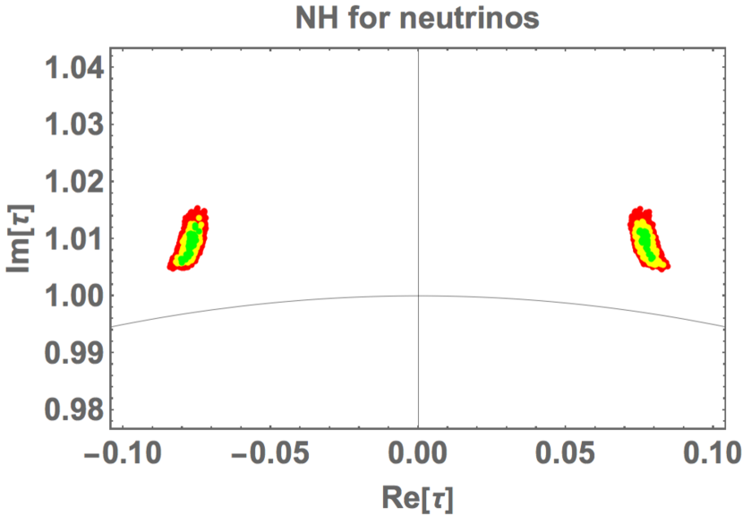
The allowed region of is restricted in the narrow regions. This result is contrast to the previous one in Ref. [75], where non-trivial phases of and enlarged the allowed region of . The predicted range of is in and at confidence level (yellow), which are close to the fixed point .
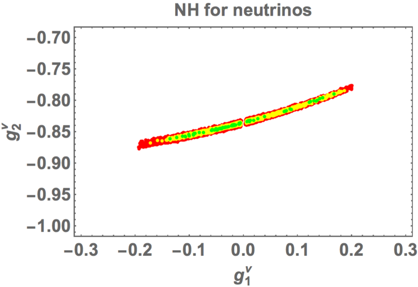
The allowed region of and is also shown in Fig. 2, where is in the rather wide region of while is restricted in at confidence level (yellow).
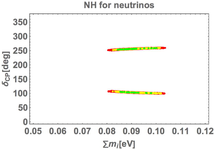
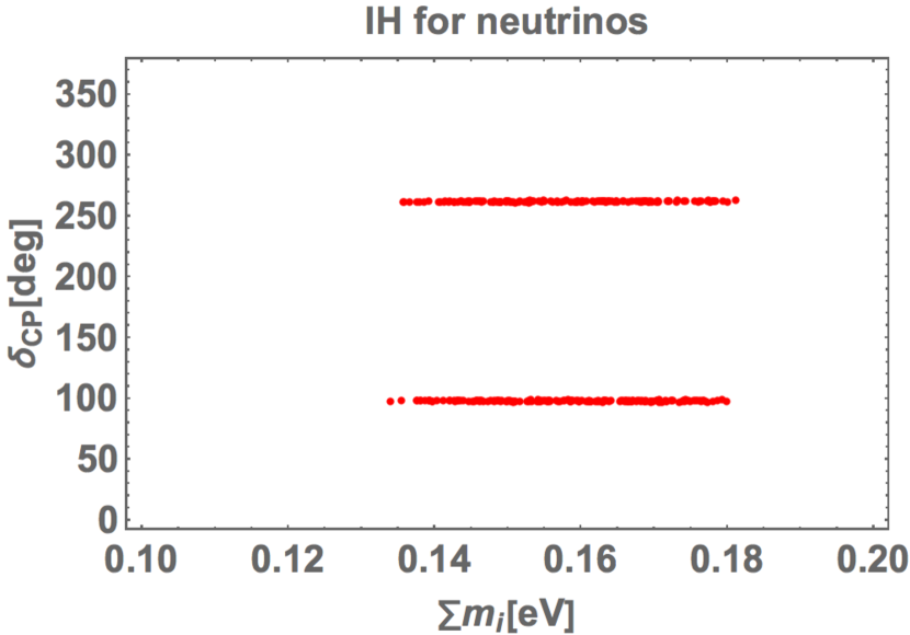
Due to restricted , the CP violating Dirac phase , which is defined in Appendix D, is predicted clearly. In Fig. 3, we show prediction of versus the sum of neutrino masses . It is remarked that is almost independent of . The predicted ranges of are narrow such as and at confidence level (yellow). The predicted ranges and correspond to – and –, respectively. The predicted is in meV for confidence level (yellow). The minimal cosmological model, , provides the upper-bound meV [117, 118]. Thus, our predicted sum of neutrino masses is consistent with the cosmological bound meV.
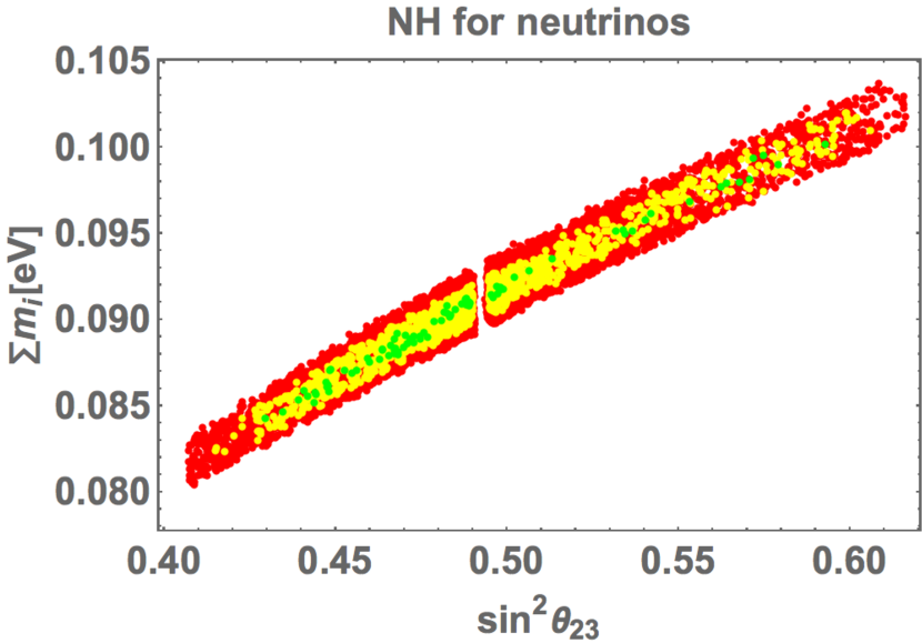
In Fig. 4, we show the allowed region on the – plane. Since depends on the value of significantly, the crucial test of our prediction will be available in the near future.
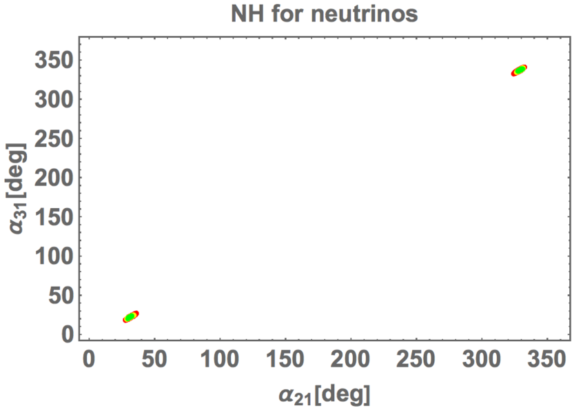
In Fig. 5, we show the prediction of Majorana phases and , which are defined by Appendix D. The predicted are around and since the source of the CP violation, is in the narrow range .
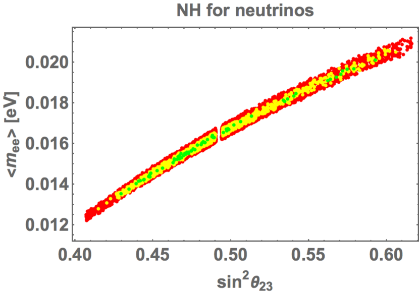
We can calculate the effective mass for the decay by using the Dirac phase and Majorana phases as seen in Appendix D. We show the predicted value of versus as seen in Fig. 6. The predicted is in meV for confidence level (yellow). The prediction of meV will be testable in the future experiments of the neutrinoless double beta decay.
It is important to understand the difference between the results in the present paper and the previous ones in Ref.[75], where imaginary parts of and also break the CP symmetry explicitly. The modulus is severely restricted around and in this work while it is allowed in rather wide region in the previous work. Indeed, the samller and the larger are allowed such as and in the previous results. Due to this restricted in this work, and the sum of neutrino masses are predicted clearly. On the other hand, the CP conservation is still allowed and could be larger than meV in the previous work. Moreover, the Dirac phase depends on .
4.2 Case of inverted hierarchy of neutrino masses
We discuss the case of IH of neutrino masses. In Fig. 7, we show the allowed region on the – plane, where the red region corresponds to confidence level like in Fig. 1. However, there are no green and yellow regions of and confidence levels.
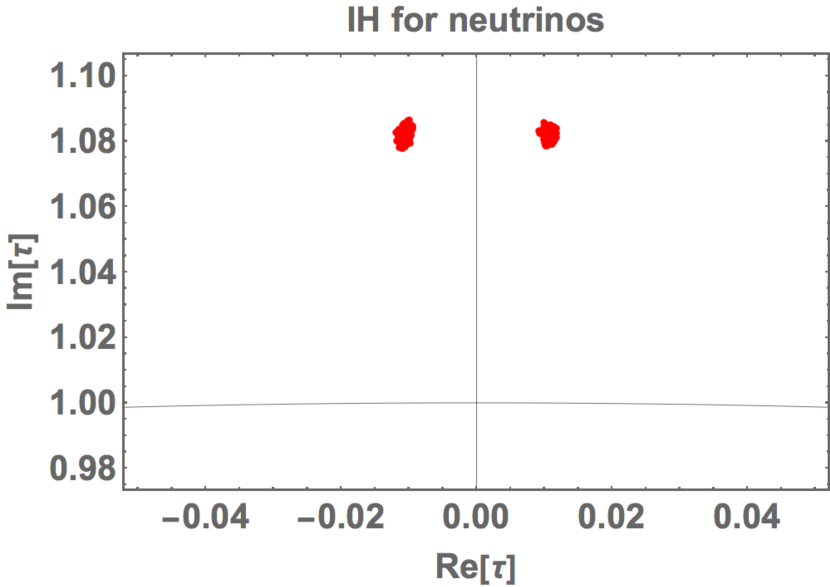
The range of is in and at confidence level, which are close to .
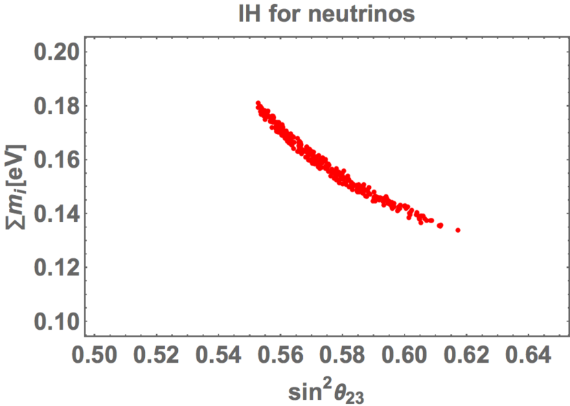
The allowed region of and is also shown in Fig. 8, where is restricted in the narrow range of while is rather large as in for .
In Fig. 9, we show prediction of versus . It is remarked that is almost independent of . The predicted range of is in and at confidence level while the sum of neutrino masses are in the range of meV. In our numerical result, there is no region of the sum of neutrino masses less than meV. The upper-bound of the minimal cosmological model, , is meV [117, 118], however, it becomes weaker when the data are analysed in the context of extended cosmological models [121]. The predicted sum of neutrino masses of IH may be still consistent with the cosmological bound.
We show the allowed region on the – plane in Fig. 10. The precise measurement of will provide a severe test for our prediction since is obtained for IH.
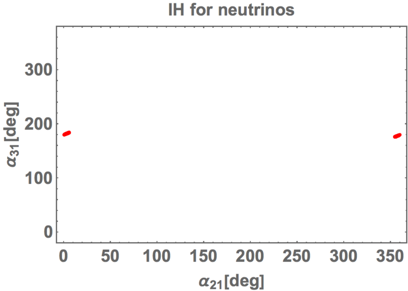
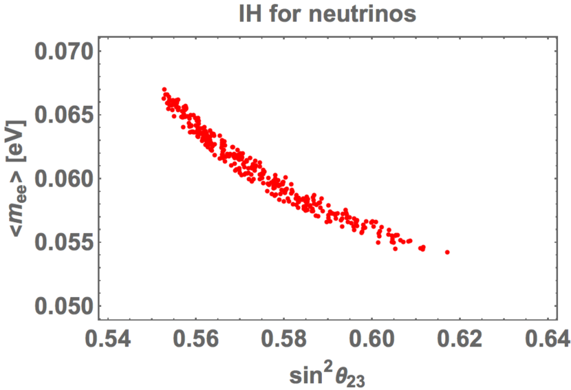
In Fig. 11, we show the prediction of Majorana phases and . The predicted are restricted around and . We also show the predicted value of versus as seen in Fig. 12. The predicted is in meV for confidence level.
As well as the case of NH, we comment on the difference between the results in the present paper and the previous ones in Ref.[75], where and are complex. Our results are obtained at more than confidence level, on the other hand, the previous ones are at less than confidence level. The modulus is also severely restricted in this work while it is allowed in rather wide region in the previous work. The sum of neutrino masses is lager than meV in this work, on the other hand, it is allowed to be smaller than meV in the previous work. For example, it could be meV, and the Dirac phase depends on .
4.3 Parameter samples of NH and IH
We show the numerical result of two samples for NH and IH, respectively. In Table 3, parameters and outputs of our calculations are presented for both NH and IH.
| NH | IH | |
|---|---|---|
| -1.17 | ||
| 6.79 | ||
| meV | meV | |
| meV | meV | |
We also present the mixing matrices of charged leptons and neutrinos for the samples of Table 3. For NH, those are:
| (36) |
which are given in the diagonal base of the generator in order to see the hierarchical structure of flavor mixing [75]. The PMNS mixing matrix is given as . The diagonal base of is obtained by using the following unitary matrix:
| (37) |
which leads to [75]. Then, the charged lepton and neutrino mass matrices are transformed as .
For IH, the mixing matrices are:
| (38) |
which are also given in the diagonal base of the generator .
For both NH and IH, the mixing matrix of charged leptons is hierarchical one, on the other hand, two large mixing angles of 1–2 and 2–3 flavors appear in the neutrino mixing matrix .
In our numerical calculations, we have not included the RGE effects in the lepton mixing angles and neutrino mass ratio . We suppose that those corrections are very small between the electroweak and GUT scales. This assumption is justified well in the case of unless neutrino masses are almost degenerate [27].
5 Summary and discussions
The modular invariant model of lepton flavors has been studied combining with the generalized CP symmetry. In our model, both CP and modular symmetries are broken spontaneously by VEV of the modulus . The source of the CP violation is a non-trivial value of while parameters of neutrinos and are real.
We have found allowed region of close to the fixed point , which is consistent with the observed lepton mixing angles and lepton masses for NH at confidence level. The CP violating Dirac phase is predicted clearly in and at confidence level. The predicted is in meV with confidence level.
There is also allowed region of close to the fixed point for IH at confidence level. The predicted is in and at confidence level. The sum of neutrino masses is predicted in meV.
By using the predicted Dirac phase and the Majorana phases, we have obtained the effective mass for the decay, which are in meV for NH at confidence level and in meV for IH at confidence level. Since KamLAND-Zen experiment [122] presented the upper bound on the effective Majorana mass as – meV by using a variety of nuclear matrix element calculations, the prediction of meV for IH will be tested in the near future. Furthermore, the prediction of meV for NH will be also testable in the future experiments of the neutrinoless double beta decay.
Since the CP symmetry is conserved at the boundary of the fundamental domain, one may expect the size of CP violation to be small at the nearby fixed point of . In order to estimate of the size of CP violation, we can calculate the rephasing invariant CP violating measure of leptons, [123, 124] from mass matrices directly [125]. By using aproximate forms of lepton mass matrices at nearby fixed points in Ref.[75], we have obtained the relation between the magnitude of and the deviation from semi-quantitatively. In order to reproduce the almost maximal size , it is enough to take where is supposed to be real in the definition of . Since it is important to study CP violation at nearby fixed points complehensively, we will present appropriate forms in another paper.
In our model, the modulus dominates the CP violation. Therefore, the determination of is the most important work. Although we have constrained by observables of leptons phenomenologically, one also should pay attention to the recent theoretical work of the moduli stabilization from the viewpoint of modular flavor symmetries [126]. The study of modulus is interesting to reveal the flavor theory in both theoretical and phenomenological aspects.
Acknowledgments
This research was supported by an appointment to the JRG Program at the APCTP through the Science and Technology Promotion Fund and Lottery Fund of the Korean Government. This was also supported by the Korean Local Governments - Gyeongsangbuk-do Province and Pohang City (H.O.). H. O. is sincerely grateful for the KIAS member.
Appendix
Appendix A Tensor product of group
Appendix B Modular forms in symmetry
For , the dimension of the linear space of modular forms of weight is [111, 112, 113], i.e., there are three linearly independent modular forms of the lowest non-trivial weight . These forms have been explicitly obtained [22] in terms of the Dedekind eta-function :
| (42) |
where is a so called modular form of weight . In what follows we will use the following base of the generators and in the triplet representation:
| (43) |
where . The modular forms of weight 2 transforming as a triplet of , , can be written in terms of and its derivative [22]:
| (44) | |||||
The overall coefficient in Eq. (44) is one possible choice. It cannot be uniquely determined. The triplet modular forms of weight have the following -expansions:
| (45) |
They satisfy also the constraint [22]:
| (46) |
The modular forms of the higher weight, , can be obtained by the tensor products of the modular forms with weight 2, , as given in Appendix A. For weight 4, that is , there are five modular forms by the tensor product of as:
where vanishes due to the constraint of Eq. (46).
Appendix C Determination of and
The coefficients , , and in Eq.(27) are taken to be real positive without loss of generality. We show these parameters are described in terms of the modular parameter and the charged lepton masses. We rewrite the mass matrix of Eq. (27) as
| (47) |
where and . Denoting charged lepton masses , and , we have three equations as:
| (48) | ||||
| (49) | ||||
| (50) |
where . The coefficients , and depend only on ’s, where ’s are determined if the value of modulus is fixed. Those are given explicitly as follows:
Then, we obtain two equations which describe and in terms of masses and :
| (51) |
where we redefine the parameters and . After fixing charged lepton masses and , we obtain and numerically. They are related as follows:
| (52) |
Appendix D Majorana and Dirac phases and in decay
Supposing neutrinos to be Majorana particles, the PMNS matrix [95, 96] is parametrized in terms of the three mixing angles , one CP violating Dirac phase and two Majorana phases , as follows:
| (53) |
where and denote and , respectively.
The rephasing invariant CP violating measure of leptons [123, 124] is defined by the PMNS matrix elements . It is written in terms of the mixing angles and the CP violating phase as:
| (54) |
where denotes the each component of the PMNS matrix.
There are also other invariants and associated with Majorana phases
| (55) |
We can calculate , and with these relations by taking account of
| (56) |
In terms of this parametrization, the effective mass for the decay is given as follows:
| (57) |
References
- [1] F. Wilczek and A. Zee, Phys. Lett. 70B (1977) 418 Erratum: [Phys. Lett. 72B (1978) 504].
- [2] S. Pakvasa and H. Sugawara, Phys. Lett. 73B (1978) 61.
- [3] M. Fukugita, M. Tanimoto and T. Yanagida, Phys. Rev. D 57 (1998) 4429 [hep-ph/9709388].
- [4] Y. Fukuda et al. [Super-Kamiokande Collaboration], Phys. Rev. Lett. 81 (1998) 1562 [hep-ex/9807003].
- [5] G. Altarelli and F. Feruglio, Rev. Mod. Phys. 82 (2010) 2701 [arXiv:1002.0211 [hep-ph]].
- [6] H. Ishimori, T. Kobayashi, H. Ohki, Y. Shimizu, H. Okada and M. Tanimoto, Prog. Theor. Phys. Suppl. 183 (2010) 1 [arXiv:1003.3552 [hep-th]].
- [7] H. Ishimori, T. Kobayashi, H. Ohki, H. Okada, Y. Shimizu and M. Tanimoto, Lect. Notes Phys. 858 (2012) 1, Springer.
- [8] D. Hernandez and A. Y. Smirnov, Phys. Rev. D 86 (2012) 053014 [arXiv:1204.0445 [hep-ph]].
- [9] S. F. King and C. Luhn, Rept. Prog. Phys. 76 (2013) 056201 [arXiv:1301.1340 [hep-ph]].
- [10] S. F. King, A. Merle, S. Morisi, Y. Shimizu and M. Tanimoto, New J. Phys. 16, 045018 (2014) [arXiv:1402.4271 [hep-ph]].
- [11] M. Tanimoto, AIP Conf. Proc. 1666 (2015) 120002.
- [12] S. F. King, Prog. Part. Nucl. Phys. 94 (2017) 217 [arXiv:1701.04413 [hep-ph]].
- [13] S. T. Petcov, Eur. Phys. J. C 78 (2018) no.9, 709 [arXiv:1711.10806 [hep-ph]].
- [14] F. Feruglio and A. Romanino, arXiv:1912.06028 [hep-ph].
- [15] E. Ma and G. Rajasekaran, Phys. Rev. D 64, 113012 (2001) [arXiv:hep-ph/0106291].
- [16] K. S. Babu, E. Ma and J. W. F. Valle, Phys. Lett. B 552, 207 (2003) [arXiv:hep-ph/0206292].
- [17] G. Altarelli and F. Feruglio, Nucl. Phys. B 720 (2005) 64 [hep-ph/0504165].
- [18] G. Altarelli and F. Feruglio, Nucl. Phys. B 741 (2006) 215 [hep-ph/0512103].
- [19] Y. Shimizu, M. Tanimoto and A. Watanabe, Prog. Theor. Phys. 126 (2011) 81 [arXiv:1105.2929 [hep-ph]].
- [20] S. T. Petcov and A. V. Titov, Phys. Rev. D 97 (2018) no.11, 115045 [arXiv:1804.00182 [hep-ph]].
- [21] S. K. Kang, Y. Shimizu, K. Takagi, S. Takahashi and M. Tanimoto, PTEP 2018, no. 8, 083B01 (2018) [arXiv:1804.10468 [hep-ph]].
- [22] F. Feruglio, in From My Vast Repertoire …: Guido Altarelli’s Legacy, A. Levy, S. Forte, Stefano, and G. Ridolfi, eds., pp.227–266, 2019, arXiv:1706.08749 [hep-ph].
- [23] R. de Adelhart Toorop, F. Feruglio and C. Hagedorn, Nucl. Phys. B 858, 437 (2012) [arXiv:1112.1340 [hep-ph]].
- [24] T. Kobayashi, K. Tanaka and T. H. Tatsuishi, Phys. Rev. D 98 (2018) no.1, 016004 [arXiv:1803.10391 [hep-ph]].
- [25] J. T. Penedo and S. T. Petcov, Nucl. Phys. B 939 (2019) 292 [arXiv:1806.11040 [hep-ph]].
- [26] P. P. Novichkov, J. T. Penedo, S. T. Petcov and A. V. Titov, JHEP 1904 (2019) 174 [arXiv:1812.02158 [hep-ph]].
- [27] J. C. Criado and F. Feruglio, SciPost Phys. 5 (2018) no.5, 042 [arXiv:1807.01125 [hep-ph]].
- [28] T. Kobayashi, N. Omoto, Y. Shimizu, K. Takagi, M. Tanimoto and T. H. Tatsuishi, JHEP 1811 (2018) 196 [arXiv:1808.03012 [hep-ph]].
- [29] G. J. Ding, S. F. King and X. G. Liu, JHEP 1909 (2019) 074 [arXiv:1907.11714 [hep-ph]].
- [30] P. P. Novichkov, J. T. Penedo, S. T. Petcov and A. V. Titov, JHEP 1904 (2019) 005 [arXiv:1811.04933 [hep-ph]].
- [31] T. Kobayashi, Y. Shimizu, K. Takagi, M. Tanimoto and T. H. Tatsuishi, JHEP 02 (2020), 097 [arXiv:1907.09141 [hep-ph]].
- [32] X. Wang and S. Zhou, JHEP 05 (2020), 017 [arXiv:1910.09473 [hep-ph]].
- [33] G. J. Ding, S. F. King and X. G. Liu, Phys. Rev. D 100 (2019) no.11, 115005 [arXiv:1903.12588 [hep-ph]].
- [34] X. G. Liu and G. J. Ding, JHEP 1908 (2019) 134 [arXiv:1907.01488 [hep-ph]].
- [35] P. Chen, G. J. Ding, J. N. Lu and J. W. F. Valle, arXiv:2003.02734 [hep-ph].
- [36] P. P. Novichkov, J. T. Penedo and S. T. Petcov, [arXiv:2006.03058 [hep-ph]].
- [37] X. G. Liu, C. Y. Yao and G. J. Ding, [arXiv:2006.10722 [hep-ph]].
- [38] T. Kobayashi and S. Tamba, Phys. Rev. D 99 (2019) no.4, 046001 [arXiv:1811.11384 [hep-th]].
- [39] A. Baur, H. P. Nilles, A. Trautner and P. K. S. Vaudrevange, Phys. Lett. B 795 (2019) 7 [arXiv:1901.03251 [hep-th]].
- [40] G. J. Ding, S. F. King, C. C. Li and Y. L. Zhou, JHEP 08 (2020), 164 [arXiv:2004.12662 [hep-ph]].
- [41] T. Asaka, Y. Heo, T. H. Tatsuishi and T. Yoshida, JHEP 2001 (2020) 144 [arXiv:1909.06520 [hep-ph]].
- [42] T. Asaka, Y. Heo and T. Yoshida, [arXiv:2009.12120 [hep-ph]].
- [43] M. K. Behera, S. Mishra, S. Singirala and R. Mohanta, [arXiv:2007.00545 [hep-ph]].
- [44] S. Mishra, [arXiv:2008.02095 [hep-ph]].
- [45] F. J. de Anda, S. F. King and E. Perdomo, Phys. Rev. D 101 (2020) no.1, 015028 [arXiv:1812.05620 [hep-ph]].
- [46] T. Kobayashi, Y. Shimizu, K. Takagi, M. Tanimoto and T. H. Tatsuishi, arXiv:1906.10341 [hep-ph].
- [47] P. P. Novichkov, S. T. Petcov and M. Tanimoto, Phys. Lett. B 793 (2019) 247 [arXiv:1812.11289 [hep-ph]].
- [48] I. de Medeiros Varzielas, S. F. King and Y. L. Zhou, Phys. Rev. D 101 (2020) no.5, 055033 [arXiv:1906.02208 [hep-ph]].
- [49] T. Kobayashi, Y. Shimizu, K. Takagi, M. Tanimoto, T. H. Tatsuishi and H. Uchida, Phys. Lett. B 794 (2019) 114 [arXiv:1812.11072 [hep-ph]].
- [50] H. Okada and M. Tanimoto, Phys. Lett. B 791 (2019) 54 [arXiv:1812.09677 [hep-ph]].
- [51] H. Okada and M. Tanimoto, arXiv:1905.13421 [hep-ph].
- [52] T. Nomura and H. Okada, Phys. Lett. B 797 (2019) 134799 [arXiv:1904.03937 [hep-ph]].
- [53] H. Okada and Y. Orikasa, Phys. Rev. D 100 (2019) no.11, 115037 [arXiv:1907.04716 [hep-ph]].
- [54] Y. Kariyazono, T. Kobayashi, S. Takada, S. Tamba and H. Uchida, Phys. Rev. D 100 (2019) no.4, 045014 [arXiv:1904.07546 [hep-th]].
- [55] T. Nomura and H. Okada, arXiv:1906.03927 [hep-ph].
- [56] H. Okada and Y. Orikasa, arXiv:1908.08409 [hep-ph].
- [57] T. Nomura, H. Okada and O. Popov, Phys. Lett. B 803 (2020) 135294 [arXiv:1908.07457 [hep-ph]].
- [58] J. C. Criado, F. Feruglio and S. J. D. King, JHEP 2002 (2020) 001 [arXiv:1908.11867 [hep-ph]].
- [59] S. F. King and Y. L. Zhou, Phys. Rev. D 101 (2020) no.1, 015001 [arXiv:1908.02770 [hep-ph]].
- [60] G. J. Ding, S. F. King, X. G. Liu and J. N. Lu, JHEP 1912 (2019) 030 [arXiv:1910.03460 [hep-ph]].
- [61] I. de Medeiros Varzielas, M. Levy and Y. L. Zhou, [arXiv:2008.05329 [hep-ph]].
- [62] D. Zhang, Nucl. Phys. B 952 (2020) 114935 [arXiv:1910.07869 [hep-ph]].
- [63] T. Nomura, H. Okada and S. Patra, arXiv:1912.00379 [hep-ph].
- [64] T. Kobayashi, T. Nomura and T. Shimomura, Phys. Rev. D 102 (2020) no.3, 035019 [arXiv:1912.00637 [hep-ph]].
- [65] J. N. Lu, X. G. Liu and G. J. Ding, Phys. Rev. D 101 (2020) no.11, 115020 [arXiv:1912.07573 [hep-ph]].
- [66] X. Wang, Nucl. Phys. B 957 (2020), 115105 [arXiv:1912.13284 [hep-ph]].
- [67] S. J. D. King and S. F. King, JHEP 09 (2020), 043 [arXiv:2002.00969 [hep-ph]].
- [68] M. Abbas, arXiv:2002.01929 [hep-ph].
- [69] H. Okada and Y. Shoji, Phys. Dark Univ. 31 (2021), 100742 [arXiv:2003.11396 [hep-ph]].
- [70] H. Okada and Y. Shoji, Nucl. Phys. B 961 (2020), 115216 [arXiv:2003.13219 [hep-ph]].
- [71] G. J. Ding and F. Feruglio, JHEP 06 (2020), 134 [arXiv:2003.13448 [hep-ph]].
- [72] T. Nomura and H. Okada, [arXiv:2007.04801 [hep-ph]].
- [73] T. Nomura and H. Okada, arXiv:2007.15459 [hep-ph].
- [74] H. Okada and M. Tanimoto, [arXiv:2005.00775 [hep-ph]].
- [75] H. Okada and M. Tanimoto, [arXiv:2009.14242 [hep-ph]].
- [76] K. I. Nagao and H. Okada, [arXiv:2008.13686 [hep-ph]].
- [77] K. I. Nagao and H. Okada, [arXiv:2010.03348 [hep-ph]].
- [78] C. Y. Yao, X. G. Liu and G. J. Ding, [arXiv:2011.03501 [hep-ph]].
- [79] X. Wang, B. Yu and S. Zhou, [arXiv:2010.10159 [hep-ph]].
- [80] M. Abbas, Phys. Atom. Nucl. 83 (2020) no.5, 764-769.
- [81] T. Kobayashi, Y. Shimizu, K. Takagi, M. Tanimoto and T. H. Tatsuishi, Phys. Rev. D 100 (2019) no.11, 115045, Erratum: [Phys. Rev. D 101 (2020) no.3, 039904] [arXiv:1909.05139 [hep-ph]].
- [82] H. P. Nilles, S. Ramos-Śanchez and P. K. S. Vaudrevange, JHEP 02 (2020), 045 [arXiv:2001.01736 [hep-ph]].
- [83] H. P. Nilles, S. Ramos-Sánchez and P. K. S. Vaudrevange, Nucl. Phys. B 957 (2020), 115098 [arXiv:2004.05200 [hep-ph]].
- [84] S. Kikuchi, T. Kobayashi, S. Takada, T. H. Tatsuishi and H. Uchida, Phys. Rev. D 102 (2020) no.10, 105010 [arXiv:2005.12642 [hep-th]].
- [85] S. Kikuchi, T. Kobayashi, H. Otsuka, S. Takada and H. Uchida, [arXiv:2007.06188 [hep-th]].
- [86] K. Ishiguro, T. Kobayashi and H. Otsuka, [arXiv:2010.10782 [hep-th]].
- [87] G. Ecker, W. Grimus and W. Konetschny, Nucl. Phys. B 191 (1981), 465-492.
- [88] G. Ecker, W. Grimus and H. Neufeld, Nucl. Phys. B 247 (1984), 70-82.
- [89] G. Ecker, W. Grimus and H. Neufeld, J. Phys. A 20 (1987), L807.
- [90] H. Neufeld, W. Grimus and G. Ecker, Int. J. Mod. Phys. A 3 (1988), 603-616.
- [91] W. Grimus and M. N. Rebelo, Phys. Rept. 281 (1997), 239-308 [arXiv:hep-ph/9506272 [hep-ph]].
- [92] W. Grimus and L. Lavoura, Phys. Lett. B 579 (2004) 113. [hep-ph/0305309].
- [93] P. P. Novichkov, J. T. Penedo, S. T. Petcov and A. V. Titov, JHEP 1907 (2019) 165 [arXiv:1905.11970 [hep-ph]].
- [94] T. Kobayashi, Y. Shimizu, K. Takagi, M. Tanimoto, T. H. Tatsuishi and H. Uchida, Phys. Rev. D 101 (2020) no.5, 055046 [arXiv:1910.11553 [hep-ph]].
- [95] Z. Maki, M. Nakagawa and S. Sakata, Prog. Theor. Phys. 28 (1962) 870.
- [96] B. Pontecorvo, Sov. Phys. JETP 26 (1968) 984 [Zh. Eksp. Teor. Fiz. 53 (1967) 1717].
- [97] K. Abe et al. [T2K Collaboration], Nature 580 (2020) 339.
- [98] P. Adamson et al. [NOvA Collaboration], Phys. Rev. Lett. 118 (2017) no.23, 231801 [arXiv:1703.03328 [hep-ex]].
- [99] G. C. Branco, R. G. Felipe and F. R. Joaquim, Rev. Mod. Phys. 84 (2012) 515 [arXiv:1111.5332 [hep-ph]].
- [100] M. Holthausen, M. Lindner and M. A. Schmidt, JHEP 1304 (2013) 122 [arXiv:1211.6953 [hep-ph]].
- [101] M. C. Chen, M. Fallbacher, K. T. Mahanthappa, M. Ratz and A. Trautner, Nucl. Phys. B 883 (2014) 267 [arXiv:1402.0507 [hep-ph]].
- [102] F. Feruglio, C. Hagedorn and R. Ziegler, JHEP 07 (2013), 027 [arXiv:1211.5560 [hep-ph]].
- [103] J. Lauer, J. Mas and H. P. Nilles, Phys. Lett. B 226, 251 (1989); Nucl. Phys. B 351, 353 (1991).
- [104] W. Lerche, D. Lust and N. P. Warner, Phys. Lett. B 231, 417 (1989).
- [105] S. Ferrara, .D. Lust and S. Theisen, Phys. Lett. B 233, 147 (1989).
- [106] D. Cremades, L. E. Ibanez and F. Marchesano, JHEP 0405, 079 (2004) [hep-th/0404229].
- [107] T. Kobayashi and S. Nagamoto, Phys. Rev. D 96, no. 9, 096011 (2017) [arXiv:1709.09784 [hep-th]].
- [108] T. Kobayashi, S. Nagamoto, S. Takada, S. Tamba and T. H. Tatsuishi, Phys. Rev. D 97, no. 11, 116002 (2018) [arXiv:1804.06644 [hep-th]].
- [109] S. Ferrara, D. Lust, A. D. Shapere and S. Theisen, Phys. Lett. B 225, 363 (1989).
- [110] M. Chen, S. Ramos-Sánchez and M. Ratz, Phys. Lett. B 801 (2020), 135153 [arXiv:1909.06910 [hep-ph]].
- [111] R. C. Gunning, Lectures on Modular Forms (Princeton University Press, Princeton, NJ, 1962).
- [112] B. Schoeneberg, Elliptic Modular Functions (Springer-Verlag, 1974).
- [113] N. Koblitz, Introduction to Elliptic Curves and Modular Forms (Springer-Verlag, 1984).
- [114] S. Antusch and V. Maurer, JHEP 1311 (2013) 115 [arXiv:1306.6879 [hep-ph]].
- [115] F. Björkeroth, F. J. de Anda, I. de Medeiros Varzielas and S. F. King, JHEP 1506 (2015) 141 [arXiv:1503.03306 [hep-ph]].
- [116] I. Esteban, M. C. Gonzalez-Garcia, M. Maltoni, T. Schwetz and A. Zhou, JHEP 09 (2020), 178 [arXiv:2007.14792 [hep-ph]].
- [117] S. Vagnozzi, E. Giusarma, O. Mena, K. Freese, M. Gerbino, S. Ho and M. Lattanzi, Phys. Rev. D 96 (2017) no.12, 123503 [arXiv:1701.08172 [astro-ph.CO]].
- [118] N. Aghanim et al. [Planck], Astron. Astrophys. 641 (2020), A6 [arXiv:1807.06209 [astro-ph.CO]].
- [119] H. Abe, T. Kobayashi, S. Uemura and J. Yamamoto, Phys. Rev. D 102 (2020) no.4, 045005 [arXiv:2003.03512 [hep-th]].
- [120] T. Kobayashi and H. Otsuka, Phys. Rev. D 102 (2020) no.2, 026004 [arXiv:2004.04518 [hep-th]].
- [121] P. A. Zyla et al. [Particle Data Group], PTEP 2020 (2020) no.8, 083C01.
- [122] A. Gando et al. [KamLAND-Zen], Phys. Rev. Lett. 117 (2016) no.8, 082503, [Addendum: Phys. Rev. Lett.117 (2016) no.10, 109903], [arXiv:1605.02889 [hep-ex]].
- [123] C. Jarlskog, Phys. Rev. Lett. 55 (1985) 1039.
- [124] P. I. Krastev and S. T. Petcov, Phys. Lett. B 205 (1988) 84.
- [125] Y. Shimizu, K. Takagi, S. Takahashi and M. Tanimoto, JHEP 04 (2019), 074 [arXiv:1901.06146 [hep-ph]].
- [126] K. Ishiguro, T. Kobayashi and H. Otsuka, [arXiv:2011.09154 [hep-ph]].