Anonymous Learning via Look-Alike Clustering: A Precise Analysis of Model Generalization

Look-alike modeling in machine learning encompasses a range of techniques that focus on identifying users who possess similar characteristics, behaviors, or preferences to a specific target individual. This approach primarily relies on the principle that individuals with shared attributes are likely to exhibit comparable interests and behaviors. By analyzing the behavior of these look-alike users, look-alike modeling enables accurate predictions for the target user. This technique has been widely used in various domains, including targeted marketing and personalized recommendations, where it plays a crucial role in enhancing user experiences and driving tailored outcomes [SGD15, MWXC16, MWW⁺16, MRH⁺11].

In this paper, we use look-alike clustering for a different purpose, namely to anonymize sensitive information of users. Consider a supervised regression setup where the training set contains $n$ pairs $({\bm{x}}_{i},\bm{y}_{i})$, for $i\in[n]$, with $y_{i}\in\mathbb{R}$ denoting the response and ${\bm{x}}_{i}\in\mathbb{R}^{d}$ representing a high-dimensional vector of features. We consider two groups of features: sensitive features, which contain some personal information about users and should be protected from the leaner, and the non-sensitive features. We assume that that the learner has access to a clustering structure on users, which is non-private information (e.g. based on non-sensitive features or other non-sensitive data set on users).

We propose a look-alike clustering approach, where we anonymize the individuals’ sensitive features by replacing them with the cluster’s average values. Only the anonymized dataset will be shared with the learner who then uses it to train a model. We refer to Figure 1 for an illustration of this approach. Note that the learner never gets access to the individuals’ sensitive features and so this approach is safe from re-identification attacks where the learner is given access to the pool of individuals’ sensitive information (up to permutation) and may use the non-sensitive features to re-identify the users. Also note that since a common representation (average sensitive features) is used for all the users in a cluster, this approach offers $m$-anonymity provided that each cluster is of size at least $m$ (minimum size clustering) [weeney2002k].

Minimum size clustering has received an increased attention mainly as a tool for anonymization and when privacy considerations are in place [BKBL07, AFK⁺05, APF⁺10]. A particular application is for providing anonymity for user targeting in online advertising with the goal of replacing the use of third-party cookies with a more privacy-respecting entity [EMMZ22]. There are a variety of approximation algorithms for clustering with minimum size constraint [PS07, DHHL17, AKBCF16, SSR21], as well as parallel and dynamic implementation [EMMZ22].

In this paper, we focus on linear regression and derive a precise characterization of model generalization³³3the ability of the model to generalize to new, unseen data from the same distribution as the training data using the look-alike clustering approach, in the so-called proportional regime where the size of training set grows in proportion to the number of parameters (which for the linear regression is equal to the number of features). The proportional regime has attracted a significant attention as overparametrized models have become greatly prevalent. It allows to understand the effect under/overparametrization in feature-rich models, providing insights to several intriguing phenomena, including double-descent behavior in the generalization error [MM22, DKT22, HJ22].

Our precise asymptotic theory allows us to demystify the effect of different factors on the model generalization under look-alike clustering, such as the role of cluster size, number of clusters, signal-to-noise ratio of the model as well as the strength of sensitive and non-sensitive features. A key tool in our analysis is a powerful extension of Gordon’s Gaussian process inequality [Gor88] known as the Convex Gaussian Minimax Theorem (CGMT), which was developed in [TOH15] and has been used for studying different learning problems; see e.g, [TAH18, DKT22, JS22, HJ22, JSH20].

Initially, it might be presumed that look-alike clustering would hinder model generalization by suppressing sensitive features of individuals, suggesting a possible tradeoff between anonymity (privacy) and model performance. However, our analysis uncovers scenarios in which look-alike clustering actually enhances model generalization! We will develop further insights on these results by arguing that the proposed look-alike clustering can serve as a form of regularization, mitigating model overfitting and consequently improving the model generalization.

Before summarizing our key contributions in this paper, we conclude this section by discussing some of the recent work on the tradeoff between privacy and model generalization at large. An approach to study such potential tradeoff is via the lens of memorization. Modern deep neural networks, with remarkable generalization property, operate in the overparametrized regime where there are more tunable parameters than the number of training samples. Such overparametrized models tend to interpolate the training data and are known to fit well even random labels [ZBH⁺21, ZBH⁺20]. Similar phenomenon has been observed in other models, such as random forest [BFLS98], Adaboost [Sch13, WOBM17], and kernel methods [BMM18, LR20]. Beyond label memorization, [BBF⁺21] studies setting where learning algorithms with near-optimal generalization must encode most of the information about the entire high-dimensional (and high-entropy) covariates of the training examples. Clearly, memorization of training data imposes significant privacy risks when this data contains sensitive personal information, and therefore these results hint to a potential trade-off between privacy protection and model generalization [SS19, FZ20, MBG21]. Lastly, [Fel20] studies settings where data is sampled from a mixture of subpopulations, and shows that label memorization is necessary for achieving near-optimal generalization error, whenever the distribution of subpopulation frequencies is long-tailed. Intuitively, this corresponds to datasets with many small distinct subpopulations. In order to predict more accurately on a subpopulation from which only a very few examples are observed, the learning algorithm needs to memorize the labels of those examples.

We consider a linear regression setting, where we are given $n$ i.i.d pairs $({\bm{x}}_{i},y_{i})$, where the response $y_{i}$ is given by

We assume that there is a clustering structure on features ${\bm{x}}_{i}$, $i\in[n]$, independent from the responses. We model this structure via Gaussian-Mixture model.

Our goal in this paper is to precisely characterize the effect of look-alike clustering on model generalization. We focus on the high-dimensional asymptotic regime, where the number of training data $n$, and features sizes $d,p$ grow in proportion.

We formalize the high-dimensional asymptotic setting in the assumption below:

To study the generalization of a model ${\bm{\theta}}$ (performance on unseen data) via the out-of-sample prediction risk defined as ${\rm Risk}({\bm{\theta}}):=\operatorname{\mathbb{E}}[(y-{\bm{x}}^{\sf T}{\bm{\theta}})^{2}]$, where $(y,{\bm{x}})$ is generated according to (2.1). Our next lemma characterizes the risk when the feature ${\bm{x}}$ is drawn from GMM.

The proof of Lemma 2.1 is deferred to the supplementary.

Consider the minimum $\ell_{2}$ norm (min-norm) least squares regression estimator of $\bm{y}$ on $\bm{X}$ defined by

where $(\bm{X}\bm{X}^{\sf T})^{\dagger}$ denotes the Moore-Penrose pseudoinverse of $\bm{X}\bm{X}^{\sf T}$. This estimator can also be formulated as

We also define the “look-alike estimator” denoted by ${\widehat{\bm{\theta}}}_{L}$, where the sensitive features are first anonymized via look-like modeling, and then the min-norm estimator is computed based on the resulting features. Specifically the sensitive feature $\bm{x}_{{\rm s}}$ of each sample is replaced by the center of its cluster. In our notation, writing $\bm{X}^{\sf T}=[\bm{X}_{{\rm s}}^{\sf T},\bm{X}_{{\rm ns}}^{\sf T}]$ , we define $\bm{X}_{L}^{\sf T}=[(\bm{M}_{{\rm s}}\bm{\Lambda})^{\sf T},\bm{X}_{{\rm ns}}^{\sf T}]$ the features matrix obtained after look-alike modeling on the sensitive features. The look-alike estimator is then given by

Our main result is to provide a precise characterization of the risk of look-alike estimator ${\widehat{\bm{\theta}}}_{L}$ as well as ${\widehat{\bm{\theta}}}$ (non-look-alike) in the asymptotic regime, as described in Assumption 1. We then discuss regimes where look-alike clustering offers better generalization.

As our analysis shows there are two majorly different setting in the behavior of the look-alike estimator:

• $(i)$

  $\psi_{d}-\psi_{p}\leq 1$. In words, the sample size $n$ is asymptotically larger than $d-p$, the number of non-sensitive features. This regime is called underparametrized asymptotics.

• $(ii)$

  $\psi_{d}-\psi_{p}\geq 1$, which is referred to as overparametrized asymptotics.

Our first theorem is on the risk of look-alike estimator in the underparametrized setting. To present our result, we consider the following singular value decomposition for $\bm{M}_{{\rm s}}$, the matrix of cluster centers restricted to sensitive features:

where $r={\rm rank}(\bm{M}_{{\rm s}})\leq k$.

There are several intriguing observations about this result. In the underparametrized regime:

1. 1.

   The risk depends on ${\bm{\theta}}_{0,{\rm s}}$ (model component on the sensitive features), only through the norms $\|{\bm{\theta}}_{0,{\rm s}}\|=r_{\rm s}$ and $\|\bm{U}_{{\rm s}}^{\sf T}{\bm{\theta}}_{0,{\rm s}}\|=\sqrt{\rho}r_{\rm s}$. Note that $\|\bm{U}_{{\rm s}}^{\sf T}{\bm{\theta}}_{0,{\rm s}}\|$ measures the alignment of the model with the left singular vectors of the cluster centers.

2. 2.

   The cluster structure on the non-sensitive features plays no role in the risk, nor does ${\bm{\theta}}_{0,{\rm ns}}$ the model component corresponding to the non-sensitive features.

3. 3.

   The cluster prior probabilities $\bm{\pi}$ does not impact the risk.

We next proceed to the overparametrized setting. For technical convenience, we make some simplifying assumption, however, we believe a similar derivation can be obtained for the general case, albeit with a more involved analysis.

Our next theorem characterizes the risk of look-alike estimator in the underparametrized regime.

As discussed in the introduction, one of the focal interest in this work is to understand cases where look-alike modeling improves generalization. In Section 5 we discuss this by comparing the look-alike estimator ${\widehat{\bm{\theta}}}_{L}$ with the min-norm estimator ${\widehat{\bm{\theta}}}$, given by (3.1) which utilizes the full information on the sensitive features. In order to do that, we next derive a precise characterization of the risk of ${\widehat{\bm{\theta}}}$ in the asymptotic setting.

In this section, we validate our theory with numerical experiments. We consider GMM with $k$ clusters, where the centers of clusters are given by $\mu\bm{u}_{\ell}$, for $\ell\in[k]$, where $\bm{u}_{\ell}\in\mathbb{R}^{d}$ are of unit $\ell_{2}$-norm. Also the vectors $\bm{u}_{\ell}$ are non-zero only on the first $p$ entries, and their restriction to these entries form a random orthogonal constellation. Therefore, defining $\bm{U}=[\bm{u}_{1},\dotsc,\bm{u}_{k}]$, we have $\bm{U}=\begin{bmatrix}\bm{U}_{{\rm s}}\\ {\mathbf{0}}\end{bmatrix}$, with $\bm{U}_{{\rm s}}^{\sf T}\bm{U}_{{\rm s}}={\bm{I}}_{k}$. In this setting there is no cluster structure on the non-sensitive features and the cluster centers on the sensitive features are orthogonal and of same norm.

Recall the decomposition of the model ${\bm{\theta}}_{0}=({\bm{\theta}}_{0,{\rm s}},{\bm{\theta}}_{0,{\rm ns}})$, with ${\bm{\theta}}_{0}$ the true underlying model (2.1) and ${\bm{\theta}}_{0,{\rm s}}$, ${\bm{\theta}}_{0,{\rm ns}}$ the components corresponding to sensitive and non-sensitive features. We generate ${\bm{\theta}}_{0,{\rm ns}}\in\mathbb{R}^{d-p}$ to have i.i.d standard normal entries and then normalize it to have $\left\|{\bm{\theta}}_{0,{\rm ns}}\right\|_{\ell_{2}}=r_{\rm ns}$. For ${\bm{\theta}}_{0,{\rm s}}$, we generate $\bm{Z}_{1},\bm{Z}_{2}\sim{\sf N}({\mathbf{0}}_{p},{\bm{I}}_{p})$, independently and let

where ${\sf P}_{\bm{U}_{{\rm s}}}:=\bm{U}_{{\rm s}}\bm{U}_{{\rm s}}^{\sf T}$ is the projection onto column space of $\bm{U}_{{\rm s}}$. Therefore, $\left\|{\bm{\theta}}_{0,{\rm s}}\right\|_{\ell_{2}}=r_{\rm s}$ and $\left\|\bm{U}_{{\rm s}}^{\sf T}{\bm{\theta}}_{0,{\rm s}}\right\|_{\ell_{2}}=\sqrt{\rho}r_{\rm s}$. Note that $\rho$ quantifies the alignment of the model with the cluster centers, confined to the sensitive features.)

We will vary the values of $r_{\rm s}$ and $r_{\rm ns}$ in our experiments. We also consider the case of balanced clusters, so the cluster prior probabilities are all equal, $\pi_{\ell}=1/k$, for $\ell\in[k]$.

We set the number of cluster $k=3$, dimension of sensitive features $p=200$ and the dimension of entire features vector $d=500$. We also set $\mu=5$ and $\rho=0.3$.

In our experiments, we vary the sample size $n$ and plot the risk of ${\widehat{\bm{\theta}}}_{L}$ and ${\widehat{\bm{\theta}}}$ versus $\psi_{d}-\psi_{p}=(d-p)/n$. We consider different settings, where we vary $r_{\rm s}$, $r_{\rm ns}$ and $\sigma$ (noise variance in model (2.1)).

In Figure 2, we report the results. Curves correspond to our asymptotic theory and does to the numerical simulations. (Each dot is obtained by averaging over 20 realizations of that configuration.) As we observe, in all scenarios our theoretical predictions are a perfect match to the empirical performance.

In Section 3, we provided a precise characterization of the risk of look-alike estimator ${\widehat{\bm{\theta}}}_{L}$ and its counterpart, the min-norm estimator ${\widehat{\bm{\theta}}}$ which utilizes the full information on the sensitive features. By virtue of these characterizations, we would like to understand regimes where the look-alike clustering helps with the model generalization, and the role of different problem parameters in achieving this improvement. Notably, since the look-alike estimator offers $m$-anonymity on the sensitive features (with $m$ the minimum size of clusters), our discussion here points out instances where data anonymization and model generalization are not in-conflict.

We define the gain of look-alike estimator $\Delta$ as follows:

which indicates the gain obtained in generalization via look-alike clustering.

For ease in presentation, we focus on the case of balanced clusters (equal priors $\pi_{1}=\dotsc=\pi_{k}=1/k$), and consider three cases:

In Figure 3(b) we report similar curves, where this time $\psi_{p}=0.5$ and we consider several values of $\rho$. As we observe, at fixed SNR the gain $\Delta$ is increasing in $\rho$. This is expected since $\rho$ measures the alignment of the underlying model ${\bm{\theta}}_{0}$ with the (left eigenvectors of) cluster centers and so higher $\rho$ is to advantage of the look-alike estimator which uses the cluster centers instead of individuals’ sensitive features.

We refer to the appendix for the proof of Theorem 5.1.

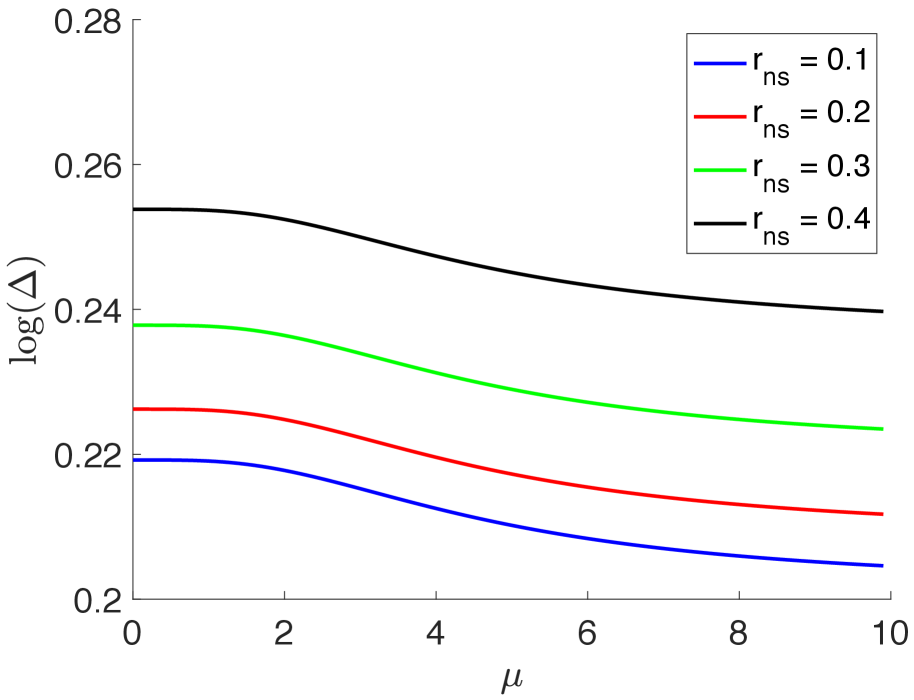
In Figure 4(a) we plot $\log(\Delta)$ versus $\mu$ for several values of $r_{\rm ns}$. Here, $\psi_{d}=2$, $\psi_{p}=1.7$, $\sigma=1$, $r_{\rm s}=0.5$ and so condition (5.1) holds. As we observe $\log(\Delta)$ is positive, decreasing in $\mu$ and also at any fixed $\mu$, it is increasing in $r_{\rm ns}$, all of which are consistent with the Theorem 5.1. In Figure 4(b), we plot similar curves where this time $r_{\rm ns}=0.2$ and we try several values of $\rho$. As we see the look-alike estimator has larger gain $\Delta$ at larger values of $\rho$.

Let us first focus on $r_{\rm ns}$, the energy of the model on the non-sensitive features. Invoking the equations (3.3) and (3.4) and hiding the terms that do not depend on $r_{\rm ns}$ in constants $C_{1}$, $C_{2}$ we arrive at

Therefore, $\lim_{r_{\rm ns}\to\infty}\Delta=(1-\psi_{d}^{-1})/(1-(\psi_{d}-\psi_{p})^{-1})>1$, indicating a gain for the look-alike estimator over ${\widehat{\bm{\theta}}}$. In Figure 5(a), we plot $\log(\Delta)$ versus $r_{\rm ns}$ for several values of $\psi_{p}$. As we observe, when $r_{\rm ns}$ is large enough we always have a gain, which is increasing in $\psi_{p}$.

We next consider the effect of SNR = $r_{\rm s}/\sigma$. In Figure 5(b) we plot $\log(\Delta)$ versus SNR, for several values of $\psi_{p}$. Similar to the underparametrized regime, we observe that in low SNR, the look-alike estimator has better generalization $(\log(\Delta)>0)$.

In previous section, we used our theory for linear models to show that at low SNR, look-alike modeling improves model generalization. We also provided an insight for this phenomenon by arguing that look-alike modeling acts as a form of regularization and avoids over-fitting at low SNR regime. In this section we show empirically that this phenomenon also extends to non-linear models.

Consider the following data generative model:

where $\varepsilon\sim{\sf N}(0,\sigma^{2})$. We construct the model ${\bm{\theta}}_{0}=({\bm{\theta}}_{0,{\rm s}},{\bm{\theta}}_{0,{\rm ns}})$ similar to the setup in Section 4. We set $n=200$, $d=180$, $k=3$, $\mu=5$, $\sigma=1$, $\rho=0.3$, $r_{\rm ns}=2$ and $N=1000$ (number of trials in Binomial distribution).

We vary SNR by changing $r_{\rm s}$ in the set $\{0.1,0.3,\dotsc,1.9\}$. The estimators ${\widehat{\bm{\theta}}}$ and ${\widehat{\bm{\theta}}}_{L}$ are obtained by fitting a GLM with logit link function and binomial distribution. We compute the risks of ${\widehat{\bm{\theta}}}$ and ${\widehat{\bm{\theta}}}_{L}$ by averaging over a test set of size $50K$. In Figure 6, we plot the gain $\log(\Delta)$ versus $r_{\rm s}$ where each data point is by averaging over $50$ different realizations of data. As we observe at low SNR, $\log(\Delta)>0$ indicating that the look-alike estimator ${\widehat{\bm{\theta}}}_{L}$ obtains a lower risk than the min-norm estimator.

Our analysis of the generalization error is based on an extension of Gordon’s Gaussian process inequality [Gor88], called Convex-Gaussian Minimax Theorem (CGMT) [TOH15]. Here, we outline the general steps of this framework and refer to the supplementary for complete details and derivations.

Consider the following two Gaussian processes:

where $\bm{G}\in\mathbb{R}^{n\times d}$, $\bm{g}\in\mathbb{R}^{n}$ and $\bm{h}\in\mathbb{R}^{d}$, all have i.i.d standard normal entries. Further, $\psi:\mathbb{R}^{d}\times\mathbb{R}^{n}\to\mathbb{R}$ is a continuous function, which is convex in the first argument and concave in the second argument.

Given the above two processes, consider the following min-max optimization problems, which are respectively referred to as the Primary Optimization (PO) and the Auxiliary Optimization (AO) problems:

The main result of CGMT is to connect the above two random optimization problems. As shown in [TOH15](Theorem 3), if $\bm{S}_{\bm{u}}$ and $\bm{S}_{\bm{v}}$ are compact and convex then, for any $\lambda\in\mathbb{R}$ and $t>0$,

An immediate corollary of this result (by choosing $\lambda=\mathbb{E}[\Phi_{\rm AO}(\bm{g},\bm{h})$]) is that if the optimal cost of the AO problem concentrates in probability, then the optimal cost of the corresponding PO problem also concentrates, in probability, around the same value. In addition, as shown in part (iii) of  [TOH15](Theorem 3), concentration of the optimal solution of the AO problem implies concentration of the optimal solution of the PO around the same value. Therefore, the two optimization are intimately connected and by analyzing the AO problem, which is substantially simpler, one can derive corresponding properties of the PO problem.

The CGMT framework has been used to infer statistical properties of estimators in certain high-dimensional asymptotic regime. The intermediate steps in the CGMT framework can be summarized as follows: First form an PO problem in the form of (7.1) and construct the corresponding AO problem. Second, derive the point-wise limit of the AO objective in terms of a convex-concave optimization problem, over only few scalar variables. This step is called ‘scalarization’. Next, it is possible to establish uniform convergence of the scalarized AO to the (deterministic) min-max optimization problem using convexity conditions. Finally, by analyzing the latter deterministic problem, one can derive the desired asymptotic characterizations.

Of course implementing the above steps involved problem-specific intricate calculations. Our proofs of Theorems 3.1, 3.2, 3.3 in the supplementary follow this general strategy.

We would like to thank Sugato Basu, Kedar Dhamdhere, Alessandro Epasto, Rezsa Farahani, Asif Islam, Omkar Muralidharan, Dustin Zelle and Peilin Zhong for helpful discussion about this work. We also thank the anonymous reviewers of NeurIPS for their thoughtful comments. This work is supported in part by the NSF CAREER Award DMS-1844481 and the NSF Award DMS-2311024.

References

• [AFK+05] Gagan Aggarwal, Tomas Feder, Krishnaram Kenthapadi, Rajeev Motwani, Rina Panigrahy, Dilys Thomas, and An Zhu, Approximation algorithms for k-anonymity, Journal of Privacy Technology 2005112001 (2005), 400.
• [AKBCF16] Faisal Abu-Khzam, Cristina Bazgan, Katrin Casel, and Henning Fernau, Building clusters with lower-bounded sizes, 27th International Symposium on Algorithms and Computation (ISAAC 2016), Schloss Dagstuhl-Leibniz-Zentrum fuer Informatik, 2016.
• [APF+10] Gagan Aggarwal, Rina Panigrahy, Tomás Feder, Dilys Thomas, Krishnaram Kenthapadi, Samir Khuller, and An Zhu, Achieving anonymity via clustering, ACM Transactions on Algorithms (TALG) 6 (2010), no. 3, 1–19.
• [BBF+21] Gavin Brown, Mark Bun, Vitaly Feldman, Adam Smith, and Kunal Talwar, When is memorization of irrelevant training data necessary for high-accuracy learning?, Proceedings of the 53rd Annual ACM SIGACT Symposium on Theory of Computing, 2021, pp. 123–132.
• [BFLS98] Peter Bartlett, Yoav Freund, Wee Sun Lee, and Robert E Schapire, Boosting the margin: A new explanation for the effectiveness of voting methods, The annals of statistics 26 (1998), no. 5, 1651–1686.
• [BKBL07] Ji-Won Byun, Ashish Kamra, Elisa Bertino, and Ninghui Li, Efficient k-anonymization using clustering techniques, Advances in Databases: Concepts, Systems and Applications: 12th International Conference on Database Systems for Advanced Applications, DASFAA 2007, Bangkok, Thailand, April 9-12, 2007. Proceedings 12, Springer, 2007, pp. 188–200.
• [BMM18] Mikhail Belkin, Siyuan Ma, and Soumik Mandal, To understand deep learning we need to understand kernel learning, International Conference on Machine Learning, PMLR, 2018, pp. 541–549.
• [DHHL17] Hu Ding, Lunjia Hu, Lingxiao Huang, and Jian Li, Capacitated center problems with two-sided bounds and outliers, Algorithms and Data Structures: 15th International Symposium, WADS 2017, St. John’s, NL, Canada, July 31–August 2, 2017, Proceedings 15, Springer, 2017, pp. 325–336.
• [DKT22] Zeyu Deng, Abla Kammoun, and Christos Thrampoulidis, A model of double descent for high-dimensional binary linear classification, Information and Inference: A Journal of the IMA 11 (2022), no. 2, 435–495.
• [EMMZ22] Alessandro Epasto, Mohammad Mahdian, Vahab Mirrokni, and Peilin Zhong, Massively parallel and dynamic algorithms for minimum size clustering, Proceedings of the 2022 Annual ACM-SIAM Symposium on Discrete Algorithms (SODA), SIAM, 2022, pp. 1613–1660.
• [Fel20] Vitaly Feldman, Does learning require memorization? a short tale about a long tail, Proceedings of the 52nd Annual ACM SIGACT Symposium on Theory of Computing, 2020, pp. 954–959.
• [FZ20] Vitaly Feldman and Chiyuan Zhang, What neural networks memorize and why: Discovering the long tail via influence estimation, Advances in Neural Information Processing Systems 33 (2020), 2881–2891.
• [Gor88] Yehoram Gordon, On milman’s inequality and random subspaces which escape through a mesh in rnr^{n}, Geometric aspects of functional analysis, Springer, 1988, pp. 84–106.
• [HJ22] Hamed Hassani and Adel Javanmard, The curse of overparametrization in adversarial training: Precise analysis of robust generalization for random features regression, arXiv preprint arXiv:2201.05149 (2022).
• [HMRT22] Trevor Hastie, Andrea Montanari, Saharon Rosset, and Ryan J Tibshirani, Surprises in high-dimensional ridgeless least squares interpolation, The Annals of Statistics 50 (2022), no. 2, 949–986.
• [JS22] Adel Javanmard and Mahdi Soltanolkotabi, Precise statistical analysis of classification accuracies for adversarial training, The Annals of Statistics 50 (2022), no. 4, 2127–2156.
• [JSH20] Adel Javanmard, Mahdi Soltanolkotabi, and Hamed Hassani, Precise tradeoffs in adversarial training for linear regression, Conference on Learning Theory, PMLR, 2020, pp. 2034–2078.
• [LR20] Tengyuan Liang and Alexander Rakhlin, Just interpolate: Kernel “ridgeless” regression can generalize, The Annals of Statistics 48 (2020), no. 3, 1329–1347.
• [MBG21] Mohammad Malekzadeh, Anastasia Borovykh, and Deniz Gündüz, Honest-but-curious nets: Sensitive attributes of private inputs can be secretly coded into the classifiers’ outputs, Proceedings of the 2021 ACM SIGSAC Conference on Computer and Communications Security, 2021, pp. 825–844.
• [MM22] Song Mei and Andrea Montanari, The generalization error of random features regression: Precise asymptotics and the double descent curve, Communications on Pure and Applied Mathematics 75 (2022), no. 4, 667–766.
• [MRH+11] Ashish Mangalampalli, Adwait Ratnaparkhi, Andrew O Hatch, Abraham Bagherjeiran, Rajesh Parekh, and Vikram Pudi, A feature-pair-based associative classification approach to look-alike modeling for conversion-oriented user-targeting in tail campaigns, Proceedings of the 20th international conference companion on World wide web, 2011, pp. 85–86.
• [MWW+16] Qiang Ma, Eeshan Wagh, Jiayi Wen, Zhen Xia, Robert Ormandi, and Datong Chen, Score look-alike audiences, 2016 IEEE 16th International Conference on Data Mining Workshops (ICDMW), IEEE, 2016, pp. 647–654.
• [MWXC16] Qiang Ma, Musen Wen, Zhen Xia, and Datong Chen, A sub-linear, massive-scale look-alike audience extension system a massive-scale look-alike audience extension, Workshop on Big Data, Streams and Heterogeneous Source Mining: Algorithms, Systems, Programming Models and Applications, PMLR, 2016, pp. 51–67.
• [PS07] Hyoungmin Park and Kyuseok Shim, Approximate algorithms for k-anonymity, Proceedings of the 2007 ACM SIGMOD international conference on Management of data, 2007, pp. 67–78.
• [Sch13] Robert E Schapire, Explaining adaboost, Empirical inference, Springer, 2013, pp. 37–52.
• [SGD15] Jianqiang Shen, Sahin Cem Geyik, and Ali Dasdan, Effective audience extension in online advertising, Proceedings of the 21th ACM SIGKDD International Conference on Knowledge Discovery and Data Mining, 2015, pp. 2099–2108.
• [SS19] Congzheng Song and Vitaly Shmatikov, Overlearning reveals sensitive attributes, arXiv preprint arXiv:1905.11742 (2019).
• [SSR21] Anik Sarker, Wing-Kin Sung, and M Sohel Rahman, A linear time algorithm for the r-gathering problem on the line, Theoretical Computer Science 866 (2021), 96–106.
• [Ste77] Gilbert W Stewart, On the perturbation of pseudo-inverses, projections and linear least squares problems, SIAM review 19 (1977), no. 4, 634–662.
• [TAH18] Christos Thrampoulidis, Ehsan Abbasi, and Babak Hassibi, Precise error analysis of regularized mm-estimators in high dimensions, IEEE Transactions on Information Theory 64 (2018), no. 8, 5592–5628.
• [TOH15] Christos Thrampoulidis, Samet Oymak, and Babak Hassibi, Regularized linear regression: A precise analysis of the estimation error, Conference on Learning Theory, 2015, pp. 1683–1709.
• [Tu20] Stephen Tu, On the smallest singular value of non-centered gaussian designs, 2020.
• [WOBM17] Abraham J Wyner, Matthew Olson, Justin Bleich, and David Mease, Explaining the success of adaboost and random forests as interpolating classifiers, The Journal of Machine Learning Research 18 (2017), no. 1, 1558–1590.
• [ZBH+20] Chiyuan Zhang, Samy Bengio, Moritz Hardt, Michael C. Mozer, and Yoram Singer, Identity crisis: Memorization and generalization under extreme overparameterization, International Conference on Learning Representations, 2020.
• [ZBH+21] Chiyuan Zhang, Samy Bengio, Moritz Hardt, Benjamin Recht, and Oriol Vinyals, Understanding deep learning (still) requires rethinking generalization, Communications of the ACM 64 (2021), no. 3, 107–115.
Appendix A Proof of theorems and technical lemmas
A.1 Proof of Lemma 2.1
By substituting for yy from (2.1) in the definition of risk we obtain
Risk(𝜽)\displaystyle{\rm Risk}({\bm{\theta}}) =𝔼[(y𝒙𝖳𝜽)2]\displaystyle=\operatorname{\mathbb{E}}[(y-{\bm{x}}^{\sf T}{\bm{\theta}})^{2}]
=𝔼[(𝒙𝖳(𝜽0𝜽))2]+𝔼[𝜺2]\displaystyle=\operatorname{\mathbb{E}}[({\bm{x}}^{\sf T}({\bm{\theta}}_{0}-{\bm{\theta}}))^{2}]+\operatorname{\mathbb{E}}[\bm{\varepsilon}^{2}]
=(a)[k]π𝔼[((𝝁+𝒛)𝖳(𝜽0𝜽))2]+𝔼[𝜺2]\displaystyle\stackrel{{\scriptstyle(a)}}{{=}}\sum_{\ell\in[k]}\pi_{\ell}\operatorname{\mathbb{E}}[(({\bm{{\mu}}}_{\ell}+\bm{z})^{\sf T}({\bm{\theta}}_{0}-{\bm{\theta}}))^{2}]+\operatorname{\mathbb{E}}[\bm{\varepsilon}^{2}]
=[k]π𝔼[(𝝁𝖳(𝜽0𝜽))2]+[k]π𝜽𝜽022+σ2\displaystyle=\sum_{\ell\in[k]}\pi_{\ell}\operatorname{\mathbb{E}}[({\bm{{\mu}}}_{\ell}^{\sf T}({\bm{\theta}}_{0}-{\bm{\theta}}))^{2}]+\sum_{\ell\in[k]}\pi_{\ell}\left\|{\bm{\theta}}-{\bm{\theta}}_{0}\right\|_{\ell_{2}}^{2}+\sigma^{2}
=(b)(𝜽𝜽0)𝖳𝑴diag(𝝅)𝑴𝖳(𝜽0𝜽)+𝜽0𝜽2+σ2,\displaystyle\stackrel{{\scriptstyle(b)}}{{=}}({\bm{\theta}}-{\bm{\theta}}_{0})^{\sf T}\bm{M}\text{diag}(\bm{\pi})\bm{M}^{\sf T}({\bm{\theta}}_{0}-{\bm{\theta}})+\left\|{\bm{\theta}}_{0}-{\bm{\theta}}\right\|_{\ell_{2}}+\sigma^{2}\,,
where (a)(a) follows from the Gaussian-Mixture model (2.2) and (b)(b) holds since [k]π=1\sum_{\ell\in[k]}\pi_{\ell}=1.
A.2 Proof of Theorem 3.1 and Theorem 3.2
Recall that the look-alike estimator is defined as the min-norm estimator over the feature matrix XLX_{L}, where the look-alike representations are used instead of individual sensitive features; see (3.2).
To analyze risk of 𝜽^L{\widehat{\bm{\theta}}}_{L}, we consider the ridge regression estimator given by
𝜽^λ=argmin𝜽12n𝒚𝑿L𝖳𝜽22+λ𝜽22.{\widehat{\bm{\theta}}}_{\lambda}=\arg\min_{{\bm{\theta}}}\frac{1}{2n}\left\|\bm{y}-\bm{X}_{L}^{\sf T}{\bm{\theta}}\right\|_{\ell_{2}}^{2}+\lambda\left\|{\bm{\theta}}\right\|_{\ell_{2}}^{2}\,.
The minimum-norm estimator is given by 𝜽^L=limλ0+𝜽^λ{\widehat{\bm{\theta}}}_{L}=\lim_{\lambda\to 0^{+}}{\widehat{\bm{\theta}}}_{\lambda}.
We follow the CGMT framework explained in Section 7. Recall that
𝑿L=[𝑴s𝚲𝑴ns𝚲+𝒁ns],\bm{X}_{L}=\begin{bmatrix}\bm{M}_{{\rm s}}\bm{\Lambda}\\ \bm{M}_{{\rm ns}}\bm{\Lambda}+\bm{Z}_{{\rm ns}}\end{bmatrix}\,,
and therefore by substituting for 𝒚\bm{y}, 𝑿\bm{X}, and 𝑿L\bm{X}_{L}, we get
12n𝒚𝑿L𝖳𝜽22\displaystyle\frac{1}{2n}\left\|\bm{y}-\bm{X}_{L}^{\sf T}{\bm{\theta}}\right\|_{\ell_{2}}^{2} =12n𝜺+𝑿𝖳𝜽0𝑿L𝖳𝜽22\displaystyle=\frac{1}{2n}\left\|\bm{\varepsilon}+\bm{X}^{\sf T}{\bm{\theta}}_{0}-\bm{X}_{L}^{\sf T}{\bm{\theta}}\right\|_{\ell_{2}}^{2}
=12n𝜺+𝚲𝖳𝑴s𝖳(𝜽0,s𝜽s)+𝒁s𝖳𝜽0,s+(𝚲𝖳𝑴ns𝖳+𝒁ns𝖳)(𝜽0,ns𝜽ns)22.\displaystyle=\frac{1}{2n}\left\|\bm{\varepsilon}+\bm{\Lambda}^{\sf T}\bm{M}_{{\rm s}}^{\sf T}({\bm{\theta}}_{0,{\rm s}}-{\bm{\theta}}_{{\rm s}})+\bm{Z}_{{\rm s}}^{\sf T}{\bm{\theta}}_{0,{\rm s}}+(\bm{\Lambda}^{\sf T}\bm{M}_{{\rm ns}}^{\sf T}+\bm{Z}_{ns}^{\sf T})({\bm{\theta}}_{0,{\rm ns}}-{\bm{\theta}}_{{\rm ns}})\right\|_{\ell_{2}}^{2}\,.
We define the primary optimization loss as follows:
PO(𝜽s,𝜽ns):=12n𝜺+𝚲𝖳𝑴s𝖳(𝜽0,s𝜽s)+𝒁s𝖳𝜽0,s+(𝚲𝖳𝑴ns𝖳+𝒁ns𝖳)(𝜽0,ns𝜽ns)22+λ𝜽s22+λ𝜽ns22\mathcal{L}_{PO}({\bm{\theta}}_{{\rm s}},{\bm{\theta}}_{{\rm ns}}):=\frac{1}{2n}\left\|\bm{\varepsilon}+\bm{\Lambda}^{\sf T}\bm{M}_{{\rm s}}^{\sf T}({\bm{\theta}}_{0,{\rm s}}-{\bm{\theta}}_{{\rm s}})+\bm{Z}_{{\rm s}}^{\sf T}{\bm{\theta}}_{0,{\rm s}}+(\bm{\Lambda}^{\sf T}\bm{M}_{{\rm ns}}^{\sf T}+\bm{Z}_{ns}^{\sf T})({\bm{\theta}}_{0,{\rm ns}}-{\bm{\theta}}_{{\rm ns}})\right\|_{\ell_{2}}^{2}+\lambda\left\|{\bm{\theta}}_{{\rm s}}\right\|_{\ell_{2}}^{2}+\lambda\left\|{\bm{\theta}}_{{\rm ns}}\right\|_{\ell_{2}}^{2}
We continue by deriving the auxiliary optimization (AO) problem. By duality, we have
PO(𝜽s,𝜽ns)\displaystyle\mathcal{L}_{PO}({\bm{\theta}}_{{\rm s}},{\bm{\theta}}_{{\rm ns}}) =max𝒗1n(𝒗𝖳𝜺+𝒗𝖳𝚲𝖳𝑴s𝖳(𝜽0,s𝜽s)+𝒗𝖳𝒁s𝖳𝜽0,s+𝒗𝖳(𝚲𝖳𝑴ns𝖳+𝒁ns𝖳)(𝜽0,ns𝜽ns)𝒗222)\displaystyle=\max_{\bm{v}}\frac{1}{n}\left(\bm{v}^{\sf T}\bm{\varepsilon}+\bm{v}^{\sf T}\bm{\Lambda}^{\sf T}\bm{M}_{{\rm s}}^{\sf T}({\bm{\theta}}_{0,{\rm s}}-{\bm{\theta}}_{{\rm s}})+\bm{v}^{\sf T}\bm{Z}_{{\rm s}}^{\sf T}{\bm{\theta}}_{0,{\rm s}}+\bm{v}^{\sf T}(\bm{\Lambda}^{\sf T}\bm{M}_{{\rm ns}}^{\sf T}+\bm{Z}_{ns}^{\sf T})({\bm{\theta}}_{0,{\rm ns}}-{\bm{\theta}}_{{\rm ns}})-\frac{\left\|\bm{v}\right\|_{\ell_{2}}^{2}}{2}\right)
+λ𝜽s22+λ𝜽ns22\displaystyle\quad+\lambda\left\|{\bm{\theta}}_{{\rm s}}\right\|_{\ell_{2}}^{2}+\lambda\left\|{\bm{\theta}}_{{\rm ns}}\right\|_{\ell_{2}}^{2}
Note that the above is jointly convex in (𝜽s,𝜽ns)({\bm{\theta}}_{{\rm s}},{\bm{\theta}}_{{\rm ns}}) and concave in 𝒗\bm{v}, and the Gaussian matrix 𝒁\bm{Z} is independent of everything else. Therefore, the AO problem reads:
AO(𝜽s,𝜽ns)\displaystyle\mathcal{L}_{AO}({\bm{\theta}}_{{\rm s}},{\bm{\theta}}_{{\rm ns}}) =max𝒗1n(𝒗𝖳𝜺+𝒗𝖳𝚲𝖳𝑴s𝖳(𝜽0,s𝜽s)\displaystyle=\max_{\bm{v}}\frac{1}{n}\Big{(}\bm{v}^{\sf T}\bm{\varepsilon}+\bm{v}^{\sf T}\bm{\Lambda}^{\sf T}\bm{M}_{{\rm s}}^{\sf T}({\bm{\theta}}_{0,{\rm s}}-{\bm{\theta}}_{{\rm s}})
+𝜽0,s2𝒈s𝖳𝒗+𝒗2𝒉s𝖳𝜽0,s\displaystyle\quad\quad\quad\quad+\left\|{\bm{\theta}}_{0,{\rm s}}\right\|_{\ell_{2}}\bm{g}_{{\rm s}}^{\sf T}\bm{v}+\left\|\bm{v}\right\|_{\ell_{2}}\bm{h}_{{\rm s}}^{\sf T}{\bm{\theta}}_{0,{\rm s}}
+𝜽0,ns𝜽ns2𝒈ns𝖳𝒗+𝒗2𝒉ns𝖳(𝜽0,ns𝜽ns)\displaystyle\quad\quad\quad\quad+\left\|{\bm{\theta}}_{0,{\rm ns}}-{\bm{\theta}}_{{\rm ns}}\right\|_{\ell_{2}}\bm{g}_{{\rm ns}}^{\sf T}\bm{v}+\left\|\bm{v}\right\|_{\ell_{2}}\bm{h}_{{\rm ns}}^{\sf T}({\bm{\theta}}_{0,{\rm ns}}-{\bm{\theta}}_{{\rm ns}})
+𝒗𝖳𝚲𝖳𝑴ns𝖳(𝜽0,ns𝜽ns)𝒗222)+λ𝜽s22+λ𝜽ns22,\displaystyle\quad\quad\quad\quad+\bm{v}^{\sf T}\bm{\Lambda}^{\sf T}\bm{M}_{{\rm ns}}^{\sf T}({\bm{\theta}}_{0,{\rm ns}}-{\bm{\theta}}_{{\rm ns}})-\frac{\left\|\bm{v}\right\|_{\ell_{2}}^{2}}{2}\Big{)}+\lambda\left\|{\bm{\theta}}_{{\rm s}}\right\|_{\ell_{2}}^{2}+\lambda\left\|{\bm{\theta}}_{{\rm ns}}\right\|_{\ell_{2}}^{2}\,,
where 𝒈s,𝒈nsn\bm{g}_{{\rm s}},\bm{g}_{{\rm ns}}\in\mathbb{R}^{n} and 𝒉sp\bm{h}_{{\rm s}}\in\mathbb{R}^{p}, 𝒉nsdp\bm{h}_{{\rm ns}}\in\mathbb{R}^{d-p} are independent Gaussian random vectors with i.i.d 𝖭(0,1){\sf N}(0,1) entries.
We next fix norm of 𝒗2=β\left\|\bm{v}\right\|_{\ell_{2}}=\beta, and maximize over its direction to obtain
AO(𝜽s,𝜽ns)\displaystyle\mathcal{L}_{AO}({\bm{\theta}}_{{\rm s}},{\bm{\theta}}_{{\rm ns}}) =maxβ01n(β𝜺+𝚲𝖳𝑴s𝖳(𝜽0,s𝜽s)+𝜽0,s2𝒈s+𝜽0,ns𝜽ns2𝒈ns+𝚲𝖳𝑴ns𝖳(𝜽0,ns𝜽ns)2\displaystyle=\max_{\beta\geq 0}\frac{1}{n}\Big{(}\beta\left\|\bm{\varepsilon}+\bm{\Lambda}^{\sf T}\bm{M}_{{\rm s}}^{\sf T}({\bm{\theta}}_{0,{\rm s}}-{\bm{\theta}}_{{\rm s}})+\left\|{\bm{\theta}}_{0,{\rm s}}\right\|_{\ell_{2}}\bm{g}_{{\rm s}}+\left\|{\bm{\theta}}_{0,{\rm ns}}-{\bm{\theta}}_{{\rm ns}}\right\|_{\ell_{2}}\bm{g}_{{\rm ns}}+\bm{\Lambda}^{\sf T}\bm{M}_{{\rm ns}}^{\sf T}({\bm{\theta}}_{0,{\rm ns}}-{\bm{\theta}}_{{\rm ns}})\right\|_{\ell_{2}}
+β𝒉s𝖳𝜽0,s+β𝒉ns𝖳(𝜽0,ns𝜽ns)β22)+λ𝜽s22+λ𝜽ns22\displaystyle\quad\quad\quad\quad+\beta\bm{h}_{{\rm s}}^{\sf T}{\bm{\theta}}_{0,{\rm s}}+\beta\bm{h}_{{\rm ns}}^{\sf T}({\bm{\theta}}_{0,{\rm ns}}-{\bm{\theta}}_{{\rm ns}})-\frac{\beta^{2}}{2}\Big{)}+\lambda\left\|{\bm{\theta}}_{{\rm s}}\right\|_{\ell_{2}}^{2}+\lambda\left\|{\bm{\theta}}_{{\rm ns}}\right\|_{\ell_{2}}^{2}
=maxβ01n(β𝜺+𝚲𝖳𝑴s𝖳(𝜽0,s𝜽s)+𝚲𝖳𝑴ns𝖳(𝜽0,ns𝜽ns)+𝜽0,s22+𝜽0,ns𝜽ns22𝒈2\displaystyle=\max_{\beta\geq 0}\frac{1}{n}\Big{(}\beta\left\|\bm{\varepsilon}+\bm{\Lambda}^{\sf T}\bm{M}_{{\rm s}}^{\sf T}({\bm{\theta}}_{0,{\rm s}}-{\bm{\theta}}_{{\rm s}})+\bm{\Lambda}^{\sf T}\bm{M}_{{\rm ns}}^{\sf T}({\bm{\theta}}_{0,{\rm ns}}-{\bm{\theta}}_{{\rm ns}})+\sqrt{\left\|{\bm{\theta}}_{0,{\rm s}}\right\|_{\ell_{2}}^{2}+\left\|{\bm{\theta}}_{0,{\rm ns}}-{\bm{\theta}}_{{\rm ns}}\right\|_{\ell_{2}}^{2}}\bm{g}\right\|_{\ell_{2}}
+β𝒉s𝖳𝜽0,s+β𝒉ns𝖳(𝜽0,ns𝜽ns)β22)+λ𝜽s22+λ𝜽ns22,\displaystyle\quad\quad\quad\quad+\beta\bm{h}_{{\rm s}}^{\sf T}{\bm{\theta}}_{0,{\rm s}}+\beta\bm{h}_{{\rm ns}}^{\sf T}({\bm{\theta}}_{0,{\rm ns}}-{\bm{\theta}}_{{\rm ns}})-\frac{\beta^{2}}{2}\Big{)}+\lambda\left\|{\bm{\theta}}_{{\rm s}}\right\|_{\ell_{2}}^{2}+\lambda\left\|{\bm{\theta}}_{{\rm ns}}\right\|_{\ell_{2}}^{2}\,,
where we used that 𝒈s,𝒈nsn\bm{g}_{{\rm s}},\bm{g}_{{\rm ns}}\in\mathbb{R}^{n} have independent Gaussian entries. Here, 𝒈n\bm{g}\in\mathbb{R}^{n} has i.i.d entries from 𝖭(0,1){\sf N}(0,1). Next, note that the above optimization over β\beta has a closed form. Using the identity maxβ0(βxβ2/2)=x+2/2\max_{\beta\geq 0}(\beta x-\beta^{2}/2)=x_{+}^{2}/2, with x+=max(x,0)x_{+}=\max(x,0), we get
AO(𝜽s,𝜽ns)\displaystyle\mathcal{L}_{AO}({\bm{\theta}}_{{\rm s}},{\bm{\theta}}_{{\rm ns}}) =12n(𝜺+𝚲𝖳𝑴s𝖳(𝜽0,s𝜽s)+𝚲𝖳𝑴ns𝖳(𝜽0,ns𝜽ns)+𝜽0,s22+𝜽0,ns𝜽ns22𝒈2\displaystyle=\frac{1}{2n}\Big{(}\left\|\bm{\varepsilon}+\bm{\Lambda}^{\sf T}\bm{M}_{{\rm s}}^{\sf T}({\bm{\theta}}_{0,{\rm s}}-{\bm{\theta}}_{{\rm s}})+\bm{\Lambda}^{\sf T}\bm{M}_{{\rm ns}}^{\sf T}({\bm{\theta}}_{0,{\rm ns}}-{\bm{\theta}}_{{\rm ns}})+\sqrt{\left\|{\bm{\theta}}_{0,{\rm s}}\right\|_{\ell_{2}}^{2}+\left\|{\bm{\theta}}_{0,{\rm ns}}-{\bm{\theta}}_{{\rm ns}}\right\|_{\ell_{2}}^{2}}\bm{g}\right\|_{\ell_{2}}
+𝒉s𝖳𝜽0,s+𝒉ns𝖳(𝜽0,ns𝜽ns))+2+λ𝜽s22+λ𝜽ns22.\displaystyle\quad\quad\quad\quad+\bm{h}_{{\rm s}}^{\sf T}{\bm{\theta}}_{0,{\rm s}}+\bm{h}_{{\rm ns}}^{\sf T}({\bm{\theta}}_{0,{\rm ns}}-{\bm{\theta}}_{{\rm ns}})\Big{)}_{+}^{2}+\lambda\left\|{\bm{\theta}}_{{\rm s}}\right\|_{\ell_{2}}^{2}+\lambda\left\|{\bm{\theta}}_{{\rm ns}}\right\|_{\ell_{2}}^{2}\,. (A.1)
Scalarization of the auxiliary optimization (AO) problem. We next proceed to scalarize the AO problem. Consider the singular value decomposition
𝑴s=𝑼s𝚺s𝑽s𝖳,\bm{M}_{{\rm s}}=\bm{U}_{{\rm s}}\bm{\Sigma}_{{\rm s}}\bm{V}_{{\rm s}}^{\sf T}\,,
with 𝑼sp×r\bm{U}_{{\rm s}}\in\mathbb{R}^{p\times r}, 𝚺sr×r\bm{\Sigma}_{{\rm s}}\in\mathbb{R}^{r\times r}, 𝑽sk×r\bm{V}_{{\rm s}}\in\mathbb{R}^{k\times r}, where r=rank(𝑴s)kr={\rm rank}(\bm{M}_{{\rm s}})\leq k. Decompose 𝒒s:=𝜽0,s𝜽s\bm{q}_{{\rm s}}:={\bm{\theta}}_{0,{\rm s}}-{\bm{\theta}}_{{\rm s}} in its projections onto the space spanned by the columns 𝒖1,s,,𝒖r,s\bm{u}_{1,{\rm s}},\dotsc,\bm{u}_{r,{\rm s}} of 𝑼s\bm{U}_{{\rm s}}, and the orthogonal component:
𝒒s=i=1rαi𝒖i,s+α0𝒒s,\bm{q}_{{\rm s}}=\sum_{i=1}^{r}\alpha_{i}\bm{u}_{i,{\rm s}}+\alpha_{0}\bm{q}_{{\rm s}}^{\perp}\,,
where 𝒒s2=1\left\|\bm{q}_{{\rm s}}^{\perp}\right\|_{\ell_{2}}=1, α00\alpha_{0}\geq 0, and 𝑼s𝖳𝒒s=𝟎\bm{U}_{{\rm s}}^{\sf T}\bm{q}_{{\rm s}}^{\perp}={\mathbf{0}}. Using the shorthand 𝜶=(α1,,αr){\bm{\alpha}}=(\alpha_{1},\dotsc,\alpha_{r}), we write
𝚲𝖳𝑴s𝖳(𝜽0,s𝜽s)=𝚲𝖳𝑽s𝚺s𝑼s𝖳𝒒s=𝚲𝖳𝑽s𝚺s𝜶.\bm{\Lambda}^{\sf T}\bm{M}_{{\rm s}}^{\sf T}({\bm{\theta}}_{0,{\rm s}}-{\bm{\theta}}_{{\rm s}})=\bm{\Lambda}^{\sf T}\bm{V}_{{\rm s}}\bm{\Sigma}_{{\rm s}}\bm{U}_{{\rm s}}^{\sf T}\bm{q}_{{\rm s}}=\bm{\Lambda}^{\sf T}\bm{V}_{{\rm s}}\bm{\Sigma}_{{\rm s}}{\bm{\alpha}}\,.
In addition,
𝜽s22\displaystyle\left\|{\bm{\theta}}_{{\rm s}}\right\|_{\ell_{2}}^{2} =𝜽0,s(𝜽0,s𝜽s)22\displaystyle=\left\|{\bm{\theta}}_{0,{\rm s}}-({\bm{\theta}}_{0,{\rm s}}-{\bm{\theta}}_{{\rm s}})\right\|_{\ell_{2}}^{2}
=𝜽0,s22+𝒒s222𝜽0,s,𝒒s\displaystyle=\left\|{\bm{\theta}}_{0,{\rm s}}\right\|_{\ell_{2}}^{2}+\left\|\bm{q}_{{\rm s}}\right\|_{\ell_{2}}^{2}-2\langle{\bm{\theta}}_{0,{\rm s}},\bm{q}_{{\rm s}}\rangle
=𝜽0,s22+𝒒s222𝜽0,s,𝑼s𝜶2α0𝜽0,s,𝒒s\displaystyle=\left\|{\bm{\theta}}_{0,{\rm s}}\right\|_{\ell_{2}}^{2}+\left\|\bm{q}_{{\rm s}}\right\|_{\ell_{2}}^{2}-2\langle{\bm{\theta}}_{0,{\rm s}},\bm{U}_{{\rm s}}{\bm{\alpha}}\rangle-2\alpha_{0}\langle{\bm{\theta}}_{0,{\rm s}},\bm{q}_{{\rm s}}^{\perp}\rangle
=𝜽0,s22+𝒒s222𝑼s𝖳𝜽0,s,𝜶2α0𝜽0,s,𝒒s\displaystyle=\left\|{\bm{\theta}}_{0,{\rm s}}\right\|_{\ell_{2}}^{2}+\left\|\bm{q}_{{\rm s}}\right\|_{\ell_{2}}^{2}-2\langle\bm{U}_{{\rm s}}^{\sf T}{\bm{\theta}}_{0,{\rm s}},{\bm{\alpha}}\rangle-2\alpha_{0}\langle{\bm{\theta}}_{0,{\rm s}},\bm{q}_{{\rm s}}^{\perp}\rangle
=𝜽0,s22+(α02+𝜶22)2𝑼s𝖳𝜽0,s,𝜶2α0𝜽0,s,𝒒s.\displaystyle=\left\|{\bm{\theta}}_{0,{\rm s}}\right\|_{\ell_{2}}^{2}+(\alpha_{0}^{2}+\left\|{\bm{\alpha}}\right\|_{\ell_{2}}^{2})-2\langle\bm{U}_{{\rm s}}^{\sf T}{\bm{\theta}}_{0,{\rm s}},{\bm{\alpha}}\rangle-2\alpha_{0}\langle{\bm{\theta}}_{0,{\rm s}},\bm{q}_{{\rm s}}^{\perp}\rangle\,. (A.2)
Similarly, we define 𝒒ns=𝜽0,ns𝜽ns\bm{q}_{{\rm ns}}={\bm{\theta}}_{0,{\rm ns}}-{\bm{\theta}}_{{\rm ns}} and consider the singular value decomposition
𝑴ns=𝑼ns𝚺ns𝑽ns𝖳,\bm{M}_{{\rm ns}}=\bm{U}_{{\rm ns}}\bm{\Sigma}_{{\rm ns}}\bm{V}_{{\rm ns}}^{\sf T}\,,
with 𝑼ns(dp)×t\bm{U}_{{\rm ns}}\in\mathbb{R}^{(d-p)\times t}, 𝚺nst×t\bm{\Sigma}_{{\rm ns}}\in\mathbb{R}^{t\times t}, 𝑽nsk×t\bm{V}_{{\rm ns}}\in\mathbb{R}^{k\times t}, where t=rank(𝑴ns)kt={\rm rank}(\bm{M}_{{\rm ns}})\leq k. Decomposing 𝒒ns\bm{q}_{{\rm ns}} in its projections on the orthogonal columns 𝒖1,ns,,𝒖r,ns\bm{u}_{1,{\rm ns}},\dotsc,\bm{u}_{r,{\rm ns}} of 𝑼ns\bm{U}_{{\rm ns}}, and the orthogonal component we write
𝒒ns=i=1tγi𝒖i,ns+γ0𝒒ns,\bm{q}_{{\rm ns}}=\sum_{i=1}^{t}\gamma_{i}\bm{u}_{i,{\rm ns}}+\gamma_{0}\bm{q}_{{\rm ns}}^{\perp}\,,
with 𝒒ns2=1\left\|\bm{q}_{{\rm ns}}^{\perp}\right\|_{\ell_{2}}=1, γ00\gamma_{0}\geq 0, and 𝑼ns𝖳𝒒ns=𝟎\bm{U}_{{\rm ns}}^{\sf T}\bm{q}_{{\rm ns}}^{\perp}={\mathbf{0}}. Define 𝜸=(γ1,,γt){\bm{\gamma}}=(\gamma_{1},\dotsc,\gamma_{t}). In this notation, we have
𝚲𝖳𝑴ns𝖳(𝜽0,ns𝜽ns)=𝚲𝖳𝑽ns𝚺ns𝑼ns𝖳𝒒ns=𝚲𝖳𝑽ns𝚺ns𝜸.\bm{\Lambda}^{\sf T}\bm{M}_{{\rm ns}}^{\sf T}({\bm{\theta}}_{0,{\rm ns}}-{\bm{\theta}}_{{\rm ns}})=\bm{\Lambda}^{\sf T}\bm{V}_{{\rm ns}}\bm{\Sigma}_{{\rm ns}}\bm{U}_{{\rm ns}}^{\sf T}\bm{q}_{{\rm ns}}=\bm{\Lambda}^{\sf T}\bm{V}_{{\rm ns}}\bm{\Sigma}_{{\rm ns}}{\bm{\gamma}}\,.
Also, 𝜽0,ns𝜽ns2=𝒒ns2=γ02+𝜸22\left\|{\bm{\theta}}_{0,{\rm ns}}-{\bm{\theta}}_{{\rm ns}}\right\|_{\ell_{2}}=\left\|\bm{q}_{{\rm ns}}\right\|_{\ell_{2}}=\sqrt{\gamma_{0}^{2}+\left\|{\bm{\gamma}}\right\|_{\ell_{2}}^{2}}. In addition,
𝒉ns𝖳(𝜽0,ns𝜽ns)\displaystyle\bm{h}_{{\rm ns}}^{\sf T}({\bm{\theta}}_{0,{\rm ns}}-{\bm{\theta}}_{{\rm ns}}) =𝒉ns𝖳𝒒ns=i=1tγi𝒉ns𝖳𝒖i,ns+γ0𝒉ns𝖳𝒒ns.\displaystyle=\bm{h}_{{\rm ns}}^{\sf T}\bm{q}_{{\rm ns}}=\sum_{i=1}^{t}\gamma_{i}\bm{h}_{{\rm ns}}^{\sf T}\bm{u}_{i,{\rm ns}}+\gamma_{0}\bm{h}_{{\rm ns}}^{\sf T}\bm{q}_{{\rm ns}}^{\perp}\,.
Using the above identities in (A.1), we have
AO(𝜽s,𝜽ns)\displaystyle\mathcal{L}_{AO}({\bm{\theta}}_{{\rm s}},{\bm{\theta}}_{{\rm ns}}) =12n(𝜺+𝚲𝖳𝑽s𝚺s𝜶+𝚲𝖳𝑽ns𝚺ns𝜸+𝜽0,s22+γ02+𝜸22𝒈2\displaystyle=\frac{1}{2n}\Big{(}\left\|\bm{\varepsilon}+\bm{\Lambda}^{\sf T}\bm{V}_{{\rm s}}\bm{\Sigma}_{{\rm s}}{\bm{\alpha}}+\bm{\Lambda}^{\sf T}\bm{V}_{{\rm ns}}\bm{\Sigma}_{{\rm ns}}{\bm{\gamma}}+\sqrt{\left\|{\bm{\theta}}_{0,{\rm s}}\right\|_{\ell_{2}}^{2}+\gamma_{0}^{2}+\left\|{\bm{\gamma}}\right\|_{\ell_{2}}^{2}}\;\bm{g}\right\|_{\ell_{2}}
+𝒉s𝖳𝜽0,s+i=1tγi𝒉ns𝖳𝒖i,ns+γ0𝒉ns𝖳𝒒ns)+2\displaystyle\quad\quad\quad+\bm{h}_{{\rm s}}^{\sf T}{\bm{\theta}}_{0,{\rm s}}+\sum_{i=1}^{t}\gamma_{i}\bm{h}_{{\rm ns}}^{\sf T}\bm{u}_{i,{\rm ns}}+\gamma_{0}\bm{h}_{{\rm ns}}^{\sf T}\bm{q}_{{\rm ns}}^{\perp}\Big{)}_{+}^{2}
+λ𝜽0,s22+λ(α02+𝜶22)2λ𝑼s𝖳𝜽0,s,𝜶2λα0𝜽0,s,𝒒s\displaystyle\quad\quad\quad+\lambda\left\|{\bm{\theta}}_{0,{\rm s}}\right\|_{\ell_{2}}^{2}+\lambda(\alpha_{0}^{2}+\left\|{\bm{\alpha}}\right\|_{\ell_{2}}^{2})-2\lambda\langle\bm{U}_{{\rm s}}^{\sf T}{\bm{\theta}}_{0,{\rm s}},{\bm{\alpha}}\rangle-2\lambda\alpha_{0}\langle{\bm{\theta}}_{0,{\rm s}},\bm{q}_{{\rm s}}^{\perp}\rangle
+λ𝜽0,ns22+λ(γ02+𝜸22)2λ𝑼ns𝖳𝜽0,ns,𝜸2λγ0𝜽0,ns,𝒒ns.\displaystyle\quad\quad\quad+\lambda\left\|{\bm{\theta}}_{0,{\rm ns}}\right\|_{\ell_{2}}^{2}+\lambda(\gamma_{0}^{2}+\left\|{\bm{\gamma}}\right\|_{\ell_{2}}^{2})-2\lambda\langle\bm{U}_{{\rm ns}}^{\sf T}{\bm{\theta}}_{0,{\rm ns}},{\bm{\gamma}}\rangle-2\lambda\gamma_{0}\langle{\bm{\theta}}_{0,{\rm ns}},\bm{q}_{{\rm ns}}^{\perp}\rangle\,. (A.3)
By the above characterization, minimization over 𝜽s{\bm{\theta}}_{{\rm s}} and 𝜽ns{\bm{\theta}}_{{\rm ns}} reduces to minimization over α0,γ0\alpha_{0},\gamma_{0}, 𝜶{\bm{\alpha}}, 𝜸{\bm{\gamma}}, 𝒒s\bm{q}_{{\rm s}}^{\perp} and 𝒒ns\bm{q}_{{\rm ns}}^{\perp}. Further, these variables are free from each other and can be optimized over separately. For 𝒒s\bm{q}_{{\rm s}}^{\perp}, there is only one term involving this variable and therefore, minimization over it reduces to
min𝒒s,𝒒s2=1𝜽0,s,𝒒s=min𝒒s,𝒒s2=1𝑼s(𝑼s)𝖳𝜽0,s,𝒒s=(𝑼s)𝖳𝜽0,s2.\min_{\bm{q}_{{\rm s}}^{\perp},\left\|\bm{q}_{{\rm s}}^{\perp}\right\|_{\ell_{2}}=1}-\langle{\bm{\theta}}_{0,{\rm s}},\bm{q}_{{\rm s}}^{\perp}\rangle=\min_{\bm{q}_{{\rm s}}^{\perp},\left\|\bm{q}_{{\rm s}}^{\perp}\right\|_{\ell_{2}}=1}-\langle\bm{U}_{{\rm s}}^{\perp}(\bm{U}_{{\rm s}}^{\perp})^{\sf T}{\bm{\theta}}_{0,{\rm s}},\bm{q}_{{\rm s}}^{\perp}\rangle=-\left\|(\bm{U}_{{\rm s}}^{\perp})^{\sf T}{\bm{\theta}}_{0,{\rm s}}\right\|_{\ell_{2}}\,.
For 𝒒ns\bm{q}_{{\rm ns}}^{\perp}, we note that there are two terms involving this variable, namely 𝒉nsn,𝒒ns\langle\frac{\bm{h}_{{\rm ns}}}{\sqrt{n}},\bm{q}_{{\rm ns}}^{\perp}\rangle and (𝑼ns)𝖳𝜽0,ns,𝒒ns\langle(\bm{U}_{{\rm ns}}^{\perp})^{\sf T}{\bm{\theta}}_{0,{\rm ns}},\bm{q}_{{\rm ns}}^{\perp}\rangle. Since 𝒒ns2=1\left\|\bm{q}_{{\rm ns}}^{\perp}\right\|_{\ell_{2}}=1, it is easy to see that the optimal 𝒒ns\bm{q}_{{\rm ns}}^{\perp} should be in the span of 𝒉ns\bm{h}_{{\rm ns}}^{\perp} and (𝑼ns)𝖳𝜽0,ns(\bm{U}_{{\rm ns}}^{\perp})^{\sf T}{\bm{\theta}}_{0,{\rm ns}}. In addition,
𝒉nsn,(𝑼ns)𝖳𝜽0,ns(p)0,\langle\frac{\bm{h}_{{\rm ns}}^{\perp}}{\sqrt{n}},(\bm{U}_{{\rm ns}}^{\perp})^{\sf T}{\bm{\theta}}_{0,{\rm ns}}\rangle\stackrel{{\scriptstyle(p)}}{{\to}}0\,,
by the law of large numbers. In words, these two vectors are asymptotically orthogonal. Hence, we can consider the following decomposition of the optimal 𝒒ns\bm{q}_{{\rm ns}}^{\perp}:
𝒒ns=ξ𝒉ns𝒉ns2+1ξ2𝑼ns(𝑼ns)𝖳𝜽0,ns(𝑼ns)𝖳𝜽0,ns2,\bm{q}_{{\rm ns}}^{\perp}=-\xi\frac{\bm{h}_{{\rm ns}}^{\perp}}{\left\|\bm{h}_{{\rm ns}}^{\perp}\right\|_{\ell_{2}}}+\sqrt{1-\xi^{2}}\frac{\bm{U}_{{\rm ns}}^{\perp}(\bm{U}_{{\rm ns}}^{\perp})^{\sf T}{\bm{\theta}}_{0,{\rm ns}}}{\left\|(\bm{U}_{{\rm ns}}^{\perp})^{\sf T}{\bm{\theta}}_{0,{\rm ns}}\right\|_{\ell_{2}}}\,,
where ξ0\xi\geq 0 and 𝒉ns\bm{h}_{{\rm ns}}^{\perp} denotes the projection of 𝒉ns\bm{h}_{{\rm ns}} onto the (left) null space of 𝑼ns\bm{U}_{{\rm ns}}. This brings us to
min𝜽s,𝜽nsAO(𝜽s,𝜽ns)\displaystyle\min_{{\bm{\theta}}_{{\rm s}},{\bm{\theta}}_{{\rm ns}}}\mathcal{L}_{AO}({\bm{\theta}}_{{\rm s}},{\bm{\theta}}_{{\rm ns}}) =minα0,γ00,𝜶,𝜸12(1n𝜺+𝚲𝖳𝑽s𝚺s𝜶+𝚲𝖳𝑽ns𝚺ns𝜸+𝜽0,s22+γ02+𝜸22𝒈2\displaystyle=\min_{\alpha_{0},\gamma_{0}\geq 0,{\bm{\alpha}},{\bm{\gamma}}}\frac{1}{2}\Big{(}\frac{1}{\sqrt{n}}\left\|\bm{\varepsilon}+\bm{\Lambda}^{\sf T}\bm{V}_{{\rm s}}\bm{\Sigma}_{{\rm s}}{\bm{\alpha}}+\bm{\Lambda}^{\sf T}\bm{V}_{{\rm ns}}\bm{\Sigma}_{{\rm ns}}{\bm{\gamma}}+\sqrt{\left\|{\bm{\theta}}_{0,{\rm s}}\right\|_{\ell_{2}}^{2}+\gamma_{0}^{2}+\left\|{\bm{\gamma}}\right\|_{\ell_{2}}^{2}}\;\bm{g}\right\|_{\ell_{2}}
+𝒉s𝖳𝜽0,sn+i=1tγi𝒉ns𝖳𝒖i,nsnγ0ξ𝒉ns2n)+2\displaystyle\quad\quad\quad+\frac{\bm{h}_{{\rm s}}^{\sf T}{\bm{\theta}}_{0,{\rm s}}}{\sqrt{n}}+\sum_{i=1}^{t}\gamma_{i}\frac{\bm{h}_{{\rm ns}}^{\sf T}\bm{u}_{i,{\rm ns}}}{\sqrt{n}}-\gamma_{0}\xi\frac{\left\|\bm{h}_{{\rm ns}}^{\perp}\right\|_{\ell_{2}}}{\sqrt{n}}\Big{)}_{+}^{2}
+λ𝜽0,s22+λ(α02+𝜶22)2λ𝑼s𝖳𝜽0,s,𝜶2λα0(𝑼s)𝖳𝜽0,s2\displaystyle\quad\quad\quad+\lambda\left\|{\bm{\theta}}_{0,{\rm s}}\right\|_{\ell_{2}}^{2}+\lambda(\alpha_{0}^{2}+\left\|{\bm{\alpha}}\right\|_{\ell_{2}}^{2})-2\lambda\langle\bm{U}_{{\rm s}}^{\sf T}{\bm{\theta}}_{0,{\rm s}},{\bm{\alpha}}\rangle-2\lambda\alpha_{0}\left\|(\bm{U}_{{\rm s}}^{\perp})^{\sf T}{\bm{\theta}}_{0,{\rm s}}\right\|_{\ell_{2}}
+λ𝜽0,ns22+λ(γ02+𝜸22)2λ𝑼ns𝖳𝜽0,ns,𝜸2λγ01ξ2(𝑼ns)𝖳𝜽0,ns2.\displaystyle\quad\quad\quad+\lambda\left\|{\bm{\theta}}_{0,{\rm ns}}\right\|_{\ell_{2}}^{2}+\lambda(\gamma_{0}^{2}+\left\|{\bm{\gamma}}\right\|_{\ell_{2}}^{2})-2\lambda\langle\bm{U}_{{\rm ns}}^{\sf T}{\bm{\theta}}_{0,{\rm ns}},{\bm{\gamma}}\rangle-2\lambda\gamma_{0}\sqrt{1-\xi^{2}}\left\|(\bm{U}_{{\rm ns}}^{\perp})^{\sf T}{\bm{\theta}}_{0,{\rm ns}}\right\|_{\ell_{2}}\,. (A.4)
Note that at this stage, the AO problem is reduced to an optimization over r+t+3r+t+3 scalar variables (α0,γ00\alpha_{0},\gamma_{0}\geq 0, 0ξ10\leq\xi\leq 1 and 𝜶r{\bm{\alpha}}\in\mathbb{R}^{r}, 𝜸t{\bm{\gamma}}\in\mathbb{R}^{t}).
Convergence of the auxiliary optimization problem. We next continue to derive the point-wise in-probability limit of the AO problem.
First observe that since 𝜺\bm{\varepsilon} and 𝒈\bm{g} are independent with i.i.d 𝖭(0,1){\sf N}(0,1) entries, we have
𝜺+𝜽0,s22+γ02+𝜸22𝒈=(d)σ2+2(𝜽0,s22+γ02+𝜸22)𝒈~,\bm{\varepsilon}+\sqrt{\left\|{\bm{\theta}}_{0,{\rm s}}\right\|_{\ell_{2}}^{2}+\gamma_{0}^{2}+\left\|{\bm{\gamma}}\right\|_{\ell_{2}}^{2}}\;\bm{g}\stackrel{{\scriptstyle(d)}}{{=}}\sqrt{\sigma^{2}+^{2}(\left\|{\bm{\theta}}_{0,{\rm s}}\right\|_{\ell_{2}}^{2}+\gamma_{0}^{2}+\left\|{\bm{\gamma}}\right\|_{\ell_{2}}^{2})}\;\tilde{\bm{g}}\,,
where 𝒈~n\tilde{\bm{g}}\in\mathbb{R}^{n} has i.i.d 𝖭(0,1){\sf N}(0,1) entries.
Second, by construction 𝚲𝚲𝖳=diag(n1,,nk)k×k\bm{\Lambda}\bm{\Lambda}^{\sf T}=\text{diag}(n_{1},\dotsc,n_{k})\in\mathbb{R}^{k\times k}, where nn_{\ell} denotes the number of examples from cluster \ell. Hence,
1n𝚲𝖳𝑽s𝚺s𝜶+𝚲𝖳𝑽ns𝚺ns𝜸22\displaystyle\frac{1}{n}\left\|\bm{\Lambda}^{\sf T}\bm{V}_{{\rm s}}\bm{\Sigma}_{{\rm s}}{\bm{\alpha}}+\bm{\Lambda}^{\sf T}\bm{V}_{{\rm ns}}\bm{\Sigma}_{{\rm ns}}{\bm{\gamma}}\right\|_{\ell_{2}}^{2} =(𝑽s𝚺s𝜶+𝑽ns𝚺ns𝜸)𝖳diag(n1n,,nkk)(𝑽s𝚺s𝜶+𝑽ns𝚺ns𝜸)\displaystyle=(\bm{V}_{{\rm s}}\bm{\Sigma}_{{\rm s}}{\bm{\alpha}}+\bm{V}_{{\rm ns}}\bm{\Sigma}_{{\rm ns}}{\bm{\gamma}})^{\sf T}\text{diag}(\tfrac{n_{1}}{n},\dotsc,\tfrac{n_{k}}{k})(\bm{V}_{{\rm s}}\bm{\Sigma}_{{\rm s}}{\bm{\alpha}}+\bm{V}_{{\rm ns}}\bm{\Sigma}_{{\rm ns}}{\bm{\gamma}})
(p)(𝑽s𝚺s𝜶+𝑽ns𝚺ns𝜸)𝖳diag(𝝅)(𝑽s𝚺s𝜶+𝑽ns𝚺ns𝜸)\displaystyle\stackrel{{\scriptstyle(p)}}{{\to}}(\bm{V}_{{\rm s}}\bm{\Sigma}_{{\rm s}}{\bm{\alpha}}+\bm{V}_{{\rm ns}}\bm{\Sigma}_{{\rm ns}}{\bm{\gamma}})^{\sf T}\text{diag}(\bm{\pi})(\bm{V}_{{\rm s}}\bm{\Sigma}_{{\rm s}}{\bm{\alpha}}+\bm{V}_{{\rm ns}}\bm{\Sigma}_{{\rm ns}}{\bm{\gamma}})
Next, by using concentration of Lipschitz functions of Gaussian vectors, we obtain
1n𝜺+𝚲𝖳𝑽s𝚺s𝜶+𝚲𝖳𝑽ns𝚺ns𝜸+𝜽0,s22+γ02+𝜸22𝒈2\displaystyle\frac{1}{\sqrt{n}}\left\|\bm{\varepsilon}+\bm{\Lambda}^{\sf T}\bm{V}_{{\rm s}}\bm{\Sigma}_{{\rm s}}{\bm{\alpha}}+\bm{\Lambda}^{\sf T}\bm{V}_{{\rm ns}}\bm{\Sigma}_{{\rm ns}}{\bm{\gamma}}+\sqrt{\left\|{\bm{\theta}}_{0,{\rm s}}\right\|_{\ell_{2}}^{2}+\gamma_{0}^{2}+\left\|{\bm{\gamma}}\right\|_{\ell_{2}}^{2}}\;\bm{g}\right\|_{\ell_{2}}
p(𝑽s𝚺s𝜶+𝑽ns𝚺ns𝜸)𝖳diag(𝝅)(𝑽s𝚺s𝜶+𝑽ns𝚺ns𝜸)+σ2+(𝜽0,s22+γ02+𝜸22)\displaystyle\stackrel{{\scriptstyle p}}{{\to}}\sqrt{(\bm{V}_{{\rm s}}\bm{\Sigma}_{{\rm s}}{\bm{\alpha}}+\bm{V}_{{\rm ns}}\bm{\Sigma}_{{\rm ns}}{\bm{\gamma}})^{\sf T}\text{diag}(\bm{\pi})(\bm{V}_{{\rm s}}\bm{\Sigma}_{{\rm s}}{\bm{\alpha}}+\bm{V}_{{\rm ns}}\bm{\Sigma}_{{\rm ns}}{\bm{\gamma}})+\sigma^{2}+(\left\|{\bm{\theta}}_{0,{\rm s}}\right\|_{\ell_{2}}^{2}+\gamma_{0}^{2}+\left\|{\bm{\gamma}}\right\|_{\ell_{2}}^{2})}
Also, since 𝜽0,s2\left\|{\bm{\theta}}_{0,{\rm s}}\right\|_{\ell_{2}} is bounded and 𝒖i,s2=1\left\|\bm{u}_{i,{\rm s}}\right\|_{\ell_{2}}=1, we get
𝒉s𝖳𝜽0,sn,𝒉ns𝖳𝒖i,nsn(p)0.\frac{\bm{h}_{{\rm s}}^{\sf T}{\bm{\theta}}_{0,{\rm s}}}{\sqrt{n}},\frac{\bm{h}_{{\rm ns}}^{\sf T}\bm{u}_{i,{\rm ns}}}{\sqrt{n}}\stackrel{{\scriptstyle(p)}}{{\to}}0\,.
In addition, 𝒉ns2\left\|\bm{h}_{{\rm ns}}^{\perp}\right\|_{\ell_{2}} concentrates around dpt\sqrt{d-p-t} and (dpt)/nψdψp(d-p-t)/n\to\psi_{d}-\psi_{p}, because tkt\leq k remains bounded as nn diverges, and so
𝒉ns2n(p)ψdψp.\frac{\left\|\bm{h}_{{\rm ns}}^{\perp}\right\|_{\ell_{2}}}{\sqrt{n}}\stackrel{{\scriptstyle(p)}}{{\to}}\sqrt{\psi_{d}-\psi_{p}}\,.
Using the above limits, the objective in (A.4) converges in-probability to
𝒟(α0,γ0,ξ,𝜶,𝜸):=\displaystyle\mathcal{D}(\alpha_{0},\gamma_{0},\xi,{\bm{\alpha}},{\bm{\gamma}}):=
12((𝑽s𝚺s𝜶+𝑽ns𝚺ns𝜸)𝖳diag(𝝅)(𝑽s𝚺s𝜶+𝑽ns𝚺ns𝜸)+σ2+(𝜽0,s22+γ02+𝜸22)γ0ξψdψp)+2\displaystyle\frac{1}{2}\left(\sqrt{(\bm{V}_{{\rm s}}\bm{\Sigma}_{{\rm s}}{\bm{\alpha}}+\bm{V}_{{\rm ns}}\bm{\Sigma}_{{\rm ns}}{\bm{\gamma}})^{\sf T}\text{diag}(\bm{\pi})(\bm{V}_{{\rm s}}\bm{\Sigma}_{{\rm s}}{\bm{\alpha}}+\bm{V}_{{\rm ns}}\bm{\Sigma}_{{\rm ns}}{\bm{\gamma}})+\sigma^{2}+(\left\|{\bm{\theta}}_{0,{\rm s}}\right\|_{\ell_{2}}^{2}+\gamma_{0}^{2}+\left\|{\bm{\gamma}}\right\|_{\ell_{2}}^{2})}-\gamma_{0}\xi\sqrt{\psi_{d}-\psi_{p}}\right)_{+}^{2}
+λ𝜽022+λ(α02+γ02+𝜶22+𝜸22)\displaystyle+\lambda\left\|{\bm{\theta}}_{0}\right\|_{\ell_{2}}^{2}+\lambda(\alpha_{0}^{2}+\gamma_{0}^{2}+\left\|{\bm{\alpha}}\right\|_{\ell_{2}}^{2}+\left\|{\bm{\gamma}}\right\|_{\ell_{2}}^{2})
2λ(𝑼s𝖳𝜽0,s,𝜶+α0(𝑼s)𝖳𝜽0,s2+𝑼ns𝖳𝜽0,ns,𝜸+γ01ξ2(𝑼ns)𝖳𝜽0,ns2)\displaystyle-2\lambda\left(\langle\bm{U}_{{\rm s}}^{\sf T}{\bm{\theta}}_{0,{\rm s}},{\bm{\alpha}}\rangle+\alpha_{0}\left\|(\bm{U}_{{\rm s}}^{\perp})^{\sf T}{\bm{\theta}}_{0,{\rm s}}\right\|_{\ell_{2}}+\langle\bm{U}_{{\rm ns}}^{\sf T}{\bm{\theta}}_{0,{\rm ns}},{\bm{\gamma}}\rangle+\gamma_{0}\sqrt{1-\xi^{2}}\left\|(\bm{U}_{{\rm ns}}^{\perp})^{\sf T}{\bm{\theta}}_{0,{\rm ns}}\right\|_{\ell_{2}}\right) (A.5)
We are now ready to prove the theorems.
A.2.1 Proof of Theorem 3.1
Using Lemma 2.1, we have
Risk(𝜽^L)\displaystyle{\rm Risk}({\widehat{\bm{\theta}}}_{L}) =σ2+𝜽0𝜽22+(𝜽0𝜽)𝖳𝑴diag(𝝅)𝑴𝖳(𝜽0𝜽)\displaystyle=\sigma^{2}+\left\|{\bm{\theta}}_{0}-{\bm{\theta}}\right\|_{\ell_{2}}^{2}+({\bm{\theta}}_{0}-{\bm{\theta}})^{\sf T}\bm{M}\text{diag}(\bm{\pi})\bm{M}^{\sf T}({\bm{\theta}}_{0}-{\bm{\theta}})
=σ2+𝒒s22+𝒒ns22+𝒒s𝖳𝑴sdiag(𝝅)𝑴s𝖳𝒒s+𝒒ns𝖳𝑴nsdiag(𝝅)𝑴ns𝖳𝒒ns\displaystyle=\sigma^{2}+\left\|\bm{q}_{{\rm s}}\right\|_{\ell_{2}}^{2}+\left\|\bm{q}_{{\rm ns}}\right\|_{\ell_{2}}^{2}+\bm{q}_{{\rm s}}^{\sf T}\bm{M}_{{\rm s}}\text{diag}(\bm{\pi})\bm{M}_{{\rm s}}^{\sf T}\bm{q}_{{\rm s}}+\bm{q}_{{\rm ns}}^{\sf T}\bm{M}_{{\rm ns}}\text{diag}(\bm{\pi})\bm{M}_{{\rm ns}}^{\sf T}\bm{q}_{{\rm ns}}
=σ2+(α02+γ02+𝜶22+𝜸22)\displaystyle=\sigma^{2}+(\alpha_{0}^{2}+\gamma_{0}^{2}+\left\|{\bm{\alpha}}\right\|_{\ell_{2}}^{2}+\left\|{\bm{\gamma}}\right\|_{\ell_{2}}^{2})
+𝜶𝖳𝚺s𝑽s𝖳diag(𝝅)𝑽s𝚺s𝜶+𝜸𝖳𝚺ns𝑽ns𝖳diag(𝝅)𝑽ns𝚺ns𝜸.\displaystyle\quad+{\bm{\alpha}}^{\sf T}\bm{\Sigma}_{{\rm s}}\bm{V}_{{\rm s}}^{\sf T}\text{diag}(\bm{\pi})\bm{V}_{{\rm s}}\bm{\Sigma}_{{\rm s}}{\bm{\alpha}}+{\bm{\gamma}}^{\sf T}\bm{\Sigma}_{{\rm ns}}\bm{V}_{{\rm ns}}^{\sf T}\text{diag}(\bm{\pi})\bm{V}_{{\rm ns}}\bm{\Sigma}_{{\rm ns}}{\bm{\gamma}}\,. (A.6)
Since ψdψp1\psi_{d}-\psi_{p}\leq 1, we are in the over- determined (a.k.a underparametrized) regime. As λ0+\lambda\to 0^{+}, the terms involving λ\lambda become negligible compared to the first term in (A.5) except those that include α0\alpha_{0}, as α0\alpha_{0} is not present in the first term . Since (x)+2(x)_{+}^{2} is increasing, and
(𝑽s𝚺s𝜶+𝑽ns𝚺ns𝜸)𝖳diag(𝝅)(𝑽s𝚺s𝜶+𝑽ns𝚺ns𝜸)+𝜸220,(\bm{V}_{{\rm s}}\bm{\Sigma}_{{\rm s}}{\bm{\alpha}}+\bm{V}_{{\rm ns}}\bm{\Sigma}_{{\rm ns}}{\bm{\gamma}})^{\sf T}\text{diag}(\bm{\pi})(\bm{V}_{{\rm s}}\bm{\Sigma}_{{\rm s}}{\bm{\alpha}}+\bm{V}_{{\rm ns}}\bm{\Sigma}_{{\rm ns}}{\bm{\gamma}})+\left\|{\bm{\gamma}}\right\|_{\ell_{2}}^{2}\geq 0,
the minimum over 𝜶{\bm{\alpha}} and 𝜸{\bm{\gamma}} is achieved for 𝜶=𝟎r{\bm{\alpha}}={\mathbf{0}}\in\mathbb{R}^{r} and 𝜸=𝟎t{\bm{\gamma}}={\mathbf{0}}\in\mathbb{R}^{t}. The optimization (A.5) then reduces to
minα0,γ00,0ξ112(σ2+(𝜽0,s22+γ02)γ0ξψdψp)+2+λα022λα0(𝑼s)𝖳𝜽0,s2.\displaystyle\min_{\alpha_{0},\gamma_{0}\geq 0,0\leq\xi\leq 1}\frac{1}{2}\left(\sqrt{\sigma^{2}+(\left\|{\bm{\theta}}_{0,{\rm s}}\right\|_{\ell_{2}}^{2}+\gamma_{0}^{2})}-\gamma_{0}\xi\sqrt{\psi_{d}-\psi_{p}}\right)_{+}^{2}+\lambda\alpha_{0}^{2}-2\lambda\alpha_{0}\left\|(\bm{U}_{{\rm s}}^{\perp})^{\sf T}{\bm{\theta}}_{0,{\rm s}}\right\|_{\ell_{2}}\,. (A.7)
The optimal ξ\xi is given by ξ=1\xi=1. Also, setting derivative with respect to α0\alpha_{0} to zero we obtain the optimal α0=(𝑼s)𝖳𝜽0,s2\alpha_{0}=\left\|(\bm{U}_{{\rm s}}^{\perp})^{\sf T}{\bm{\theta}}_{0,{\rm s}}\right\|_{\ell_{2}}. Next, by setting derivative with respect to γ0\gamma_{0} we arrive at
γ02=(σ2+𝜽0,s22)ψdψp1(ψdψp).\gamma_{0}^{2}=(\sigma^{2}+\left\|{\bm{\theta}}_{0,{\rm s}}\right\|_{\ell_{2}}^{2})\frac{\psi_{d}-\psi_{p}}{1-(\psi_{d}-\psi_{p})}\,.
Using the optimal variables in (A.6) we obtain the risk of minimum-norm estimator as
Risk(𝜽^L)\displaystyle{\rm Risk}({\widehat{\bm{\theta}}}_{L}) =σ2+(𝑼s)𝖳𝜽0,s22+(σ2+𝜽0,s22)ψdψp1(ψdψp)\displaystyle=\sigma^{2}+\left\|(\bm{U}_{{\rm s}}^{\perp})^{\sf T}{\bm{\theta}}_{0,{\rm s}}\right\|_{\ell_{2}}^{2}+(\sigma^{2}+\left\|{\bm{\theta}}_{0,{\rm s}}\right\|_{\ell_{2}}^{2})\frac{\psi_{d}-\psi_{p}}{1-(\psi_{d}-\psi_{p})}
=(σ2+𝜽0,s22)11(ψdψp)𝑼s𝖳𝜽0,s22.\displaystyle=(\sigma^{2}+\left\|{\bm{\theta}}_{0,{\rm s}}\right\|_{\ell_{2}}^{2})\frac{1}{1-(\psi_{d}-\psi_{p})}-\left\|\bm{U}_{{\rm s}}^{\sf T}{\bm{\theta}}_{0,{\rm s}}\right\|_{\ell_{2}}^{2}\,.
Recall that by assumption, rs=𝜽0,s2r_{\rm s}=\left\|{\bm{\theta}}_{0,{\rm s}}\right\|_{\ell_{2}} and 𝑼s𝖳𝜽0,s2=ρrs\left\|\bm{U}_{{\rm s}}^{\sf T}{\bm{\theta}}_{0,{\rm s}}\right\|_{\ell_{2}}=\sqrt{\rho}r_{\rm s}, which completes the proof.
A.2.2 Proof of Theorem 3.2
We continue from (A.5). In the case of ψdψp1\psi_{d}-\psi_{p}\leq 1, it is easy to see that the derivative of the first term of (A.5), in the active region is decreasing in γ0\gamma_{0}. With the consideration λ0+\lambda\to 0^{+}, minimizing over γ0\gamma_{0} will push us into the non-active region. Therefore the optimization problem (A.5) reduces to
minimize𝜽022+α02+γ02+𝜶22+𝜸22\displaystyle\text{minimize}\quad\left\|{\bm{\theta}}_{0}\right\|_{\ell_{2}}^{2}+\alpha_{0}^{2}+\gamma_{0}^{2}+\left\|{\bm{\alpha}}\right\|_{\ell_{2}}^{2}+\left\|{\bm{\gamma}}\right\|_{\ell_{2}}^{2}
2(𝑼s𝖳𝜽0,s,𝜶+α0(𝑼s)𝖳𝜽0,s2+𝑼ns𝖳𝜽0,ns,𝜸+γ01ξ2(𝑼ns)𝖳𝜽0,ns2)\displaystyle\quad\quad\quad\quad\quad-2\left(\langle\bm{U}_{{\rm s}}^{\sf T}{\bm{\theta}}_{0,{\rm s}},{\bm{\alpha}}\rangle+\alpha_{0}\left\|(\bm{U}_{{\rm s}}^{\perp})^{\sf T}{\bm{\theta}}_{0,{\rm s}}\right\|_{\ell_{2}}+\langle\bm{U}_{{\rm ns}}^{\sf T}{\bm{\theta}}_{0,{\rm ns}},{\bm{\gamma}}\rangle+\gamma_{0}\sqrt{1-\xi^{2}}\left\|(\bm{U}_{{\rm ns}}^{\perp})^{\sf T}{\bm{\theta}}_{0,{\rm ns}}\right\|_{\ell_{2}}\right)
subject to
(𝑽s𝚺s𝜶+𝑽ns𝚺ns𝜸)𝖳diag(𝝅)(𝑽s𝚺s𝜶+𝑽ns𝚺ns𝜸)+σ2+(𝜽0,s22+γ02+𝜸22)γ02ξ2(ψdψp)\displaystyle(\bm{V}_{{\rm s}}\bm{\Sigma}_{{\rm s}}{\bm{\alpha}}+\bm{V}_{{\rm ns}}\bm{\Sigma}_{{\rm ns}}{\bm{\gamma}})^{\sf T}\text{diag}(\bm{\pi})(\bm{V}_{{\rm s}}\bm{\Sigma}_{{\rm s}}{\bm{\alpha}}+\bm{V}_{{\rm ns}}\bm{\Sigma}_{{\rm ns}}{\bm{\gamma}})+\sigma^{2}+(\left\|{\bm{\theta}}_{0,{\rm s}}\right\|_{\ell_{2}}^{2}+\gamma_{0}^{2}+\left\|{\bm{\gamma}}\right\|_{\ell_{2}}^{2})\leq\gamma_{0}^{2}\xi^{2}(\psi_{d}-\psi_{p}) (A.8)
By Assumption 2, 𝚺s=μ𝑰k\bm{\Sigma}_{{\rm s}}=\mu{\bm{I}}_{k}, 𝑽s=𝑰k×k\bm{V}_{{\rm s}}={\bm{I}}_{k\times k}, and 𝚺ns=𝟎\bm{\Sigma}_{{\rm ns}}={\mathbf{0}}, 𝑼ns=𝟎\bm{U}_{{\rm ns}}={\mathbf{0}} (no cluster structure on non-sensitive features and an orthogonal, equal energy cluster centers on the sensitive features). Therefore, by fixing γ:=𝜸2\gamma:=\left\|{\bm{\gamma}}\right\|_{\ell_{2}}, the optimization problem (A.8) becomes:
minimize α02+γ02+𝜶22+γ22(𝑼s𝖳𝜽0,s,𝜶+α0(𝑼s)𝖳𝜽0,s2+γ01ξ2𝜽0,ns2)\displaystyle\alpha_{0}^{2}+\gamma_{0}^{2}+\left\|{\bm{\alpha}}\right\|_{\ell_{2}}^{2}+\gamma^{2}-2\left(\langle\bm{U}_{{\rm s}}^{\sf T}{\bm{\theta}}_{0,{\rm s}},{\bm{\alpha}}\rangle+\alpha_{0}\left\|(\bm{U}_{{\rm s}}^{\perp})^{\sf T}{\bm{\theta}}_{0,{\rm s}}\right\|_{\ell_{2}}+\gamma_{0}\sqrt{1-\xi^{2}}\left\|{\bm{\theta}}_{0,{\rm ns}}\right\|_{\ell_{2}}\right)
μ2𝜶𝖳diag(𝝅)𝜶+σ2+𝜽0,s22+γ02+γ2γ02ξ2(ψdψp).\displaystyle\mu^{2}{\bm{\alpha}}^{\sf T}\text{diag}(\bm{\pi}){\bm{\alpha}}+\sigma^{2}+\left\|{\bm{\theta}}_{0,{\rm s}}\right\|_{\ell_{2}}^{2}+\gamma_{0}^{2}+\gamma^{2}\leq\gamma_{0}^{2}\xi^{2}(\psi_{d}-\psi_{p})\,. (A.9)
Since α0\alpha_{0} does not appear in the constraint, it is easy to see that its optimal value is given by α0=(𝑼s)𝖳𝜽0,s2\alpha_{0}=\left\|(\bm{U}_{{\rm s}}^{\perp})^{\sf T}{\bm{\theta}}_{0,{\rm s}}\right\|_{\ell_{2}}. Also, note that by decreasing γ\gamma the objective value decreases and also by the constraint on the other variables become more relaxed. Consequently, the optimal value of γ\gamma is γ=0\gamma=0. Removing α0\alpha_{0} from the objective function, we are left with
minimize γ02+𝜶222(𝑼s𝖳𝜽0,s,𝜶+γ01ξ2𝜽0,ns2)\displaystyle\gamma_{0}^{2}+\left\|{\bm{\alpha}}\right\|_{\ell_{2}}^{2}-2\left(\langle\bm{U}_{{\rm s}}^{\sf T}{\bm{\theta}}_{0,{\rm s}},{\bm{\alpha}}\rangle+\gamma_{0}\sqrt{1-\xi^{2}}\left\|{\bm{\theta}}_{0,{\rm ns}}\right\|_{\ell_{2}}\right)
subject to μ2𝜶𝖳diag(𝝅)𝜶+σ2+𝜽0,s22+γ02γ02ξ2(ψdψp).\displaystyle\mu^{2}{\bm{\alpha}}^{\sf T}\text{diag}(\bm{\pi}){\bm{\alpha}}+\sigma^{2}+\left\|{\bm{\theta}}_{0,{\rm s}}\right\|_{\ell_{2}}^{2}+\gamma_{0}^{2}\leq\gamma_{0}^{2}\xi^{2}(\psi_{d}-\psi_{p})\,. (A.10)
Optimal choice of ξ\xi results in the constraint to become equality. Solving for ξ\xi, the optimization reduces to
minimizeγ02+𝜶222(𝑼s𝖳𝜽0,s,𝜶+γ02μ2𝜶𝖳diag(𝝅)𝜶+σ2+𝜽0,s22+γ02ψdψp𝜽0,ns2)\displaystyle\text{minimize}\quad\gamma_{0}^{2}+\left\|{\bm{\alpha}}\right\|_{\ell_{2}}^{2}-2\left(\langle\bm{U}_{{\rm s}}^{\sf T}{\bm{\theta}}_{0,{\rm s}},{\bm{\alpha}}\rangle+\sqrt{\gamma_{0}^{2}-\frac{\mu^{2}{\bm{\alpha}}^{\sf T}\text{diag}(\bm{\pi}){\bm{\alpha}}+\sigma^{2}+\left\|{\bm{\theta}}_{0,{\rm s}}\right\|_{\ell_{2}}^{2}+\gamma_{0}^{2}}{\psi_{d}-\psi_{p}}}\left\|{\bm{\theta}}_{0,{\rm ns}}\right\|_{\ell_{2}}\right)
Setting derivative with respect to γ0\gamma_{0} to zero, we obtain
γ02μ2𝜶𝖳diag(𝝅)𝜶+σ2+𝜽0,s22+γ02ψdψp=(11ψdψp)𝜽0,ns2.\displaystyle\sqrt{\gamma_{0}^{2}-\frac{\mu^{2}{\bm{\alpha}}^{\sf T}\text{diag}(\bm{\pi}){\bm{\alpha}}+\sigma^{2}+\left\|{\bm{\theta}}_{0,{\rm s}}\right\|_{\ell_{2}}^{2}+\gamma_{0}^{2}}{\psi_{d}-\psi_{p}}}=\left(1-\frac{1}{\psi_{d}-\psi_{p}}\right)\left\|{\bm{\theta}}_{0,{\rm ns}}\right\|_{\ell_{2}}\,. (A.11)
Setting derivative with respect to 𝜶{\bm{\alpha}} to zero and using the previous stationary equation, we get
𝜶=(𝑰+μ2diag(𝝅)ψdψp1)1𝑼s𝖳𝜽0,s.\displaystyle{\bm{\alpha}}=\left({\bm{I}}+\frac{\mu^{2}\text{diag}(\bm{\pi})}{\psi_{d}-\psi_{p}-1}\right)^{-1}\bm{U}_{{\rm s}}^{\sf T}{\bm{\theta}}_{0,{\rm s}}\,. (A.12)
We next square both sides of (A.12) and rearrange the terms to get
γ02\displaystyle\gamma_{0}^{2} =1ψdψp1(σ2+𝜽0,s22+μ2𝜶𝖳diag(𝝅)𝜶)+(11ψdψp)𝜽0,ns22\displaystyle=\frac{1}{\psi_{d}-\psi_{p}-1}\left({\sigma^{2}}+\left\|{\bm{\theta}}_{0,{\rm s}}\right\|_{\ell_{2}}^{2}+\mu^{2}{\bm{\alpha}}^{\sf T}\text{diag}(\bm{\pi}){\bm{\alpha}}\right)+\left(1-\frac{1}{\psi_{d}-\psi_{p}}\right)\left\|{\bm{\theta}}_{0,{\rm ns}}\right\|_{\ell_{2}}^{2}
=1ψdψp1(σ2+rs2+μ2𝜶𝖳diag(𝝅)𝜶)+(11ψdψp)rns2,\displaystyle=\frac{1}{\psi_{d}-\psi_{p}-1}\left({\sigma^{2}}+r_{\rm s}^{2}+\mu^{2}{\bm{\alpha}}^{\sf T}\text{diag}(\bm{\pi}){\bm{\alpha}}\right)+\left(1-\frac{1}{\psi_{d}-\psi_{p}}\right)r_{\rm ns}^{2}\,,
which are the same expressions for 𝜶{\bm{\alpha}} and γ0\gamma_{0} given in the theorem statement.
The final step is to write the risk of estimator in terms of 𝜶{\bm{\alpha}}, γ0\gamma_{0}. Invoke equation (A.6), and recall that in the current case, 𝚺ns=𝟎\bm{\Sigma}_{{\rm ns}}={\mathbf{0}}, 𝚺s=μ𝑰\bm{\Sigma}_{{\rm s}}=\mu{\bm{I}}. Also, as we showed in our derivation, γ=𝜸2=0\gamma=\left\|{\bm{\gamma}}\right\|_{\ell_{2}}=0, α0=(𝑼s)𝖳𝜽0,s2\alpha_{0}=\left\|(\bm{U}_{{\rm s}}^{\perp})^{\sf T}{\bm{\theta}}_{0,{\rm s}}\right\|_{\ell_{2}}, by which we arrive at
Risk(𝜽^L)\displaystyle{\rm Risk}({\widehat{\bm{\theta}}}_{L}) =μ2𝜶𝖳diag(𝝅)𝜶+σ2+((𝑼s)𝖳𝜽0,s22+γ02+𝜶22)\displaystyle=\mu^{2}{\bm{\alpha}}^{\sf T}\text{diag}(\bm{\pi}){\bm{\alpha}}+\sigma^{2}+(\left\|(\bm{U}_{{\rm s}}^{\perp})^{\sf T}{\bm{\theta}}_{0,{\rm s}}\right\|_{\ell_{2}}^{2}+\gamma_{0}^{2}+\left\|{\bm{\alpha}}\right\|_{\ell_{2}}^{2})
=σ2+(1ρ)rs2+γ02+𝜶𝖳(𝑰+μ2diag(𝝅))𝜶.\displaystyle=\sigma^{2}+(1-\rho)r_{\rm s}^{2}+\gamma_{0}^{2}+{\bm{\alpha}}^{\sf T}\left({\bm{I}}+\mu^{2}\text{diag}(\bm{\pi})\right){\bm{\alpha}}\,. (A.13)
This concludes the proof.
A.3 Proof of Theorem 3.3
We follow the proof strategy used for Theorem 3.1-3.2. Here, we would like to characterize the risk of min-norm estimator 𝜽^{\widehat{\bm{\theta}}}. The features matrix has a clustering structure, but the learner is not using that (no look-alike clustering) and is just compute the min-norm estimator for fitting the responses to individual features. Therefore, one can think of this setting as a special case of our previous analysis when there is no sensitive features (so ψp=0\psi_{p}=0).
• (a)(a)
By setting ψp=0\psi_{p}=0 and rs=0r_{\rm s}=0 in the result of Theorem 3.1, we get that when ψd1\psi_{d}\leq 1,
Risk(𝜽^)=σ21ψd.\displaystyle{\rm Risk}({\widehat{\bm{\theta}}})=\frac{\sigma^{2}}{1-\psi_{d}}\,.
• (b)(b)
In this case, we specialize the proof of Theorem 3.2 to the case that ψp=0\psi_{p}=0. Continuing from (A.8), and removing the terms corresponding to sensitive features, we arrive at
minimize γ02+𝜸222(𝑼ns𝖳𝜽0,ns,𝜸+γ01ξ2(𝑼ns)𝖳𝜽0,ns2)\displaystyle\gamma_{0}^{2}+\left\|{\bm{\gamma}}\right\|_{\ell_{2}}^{2}-2\left(\langle\bm{U}_{{\rm ns}}^{\sf T}{\bm{\theta}}_{0,{\rm ns}},{\bm{\gamma}}\rangle+\gamma_{0}\sqrt{1-\xi^{2}}\left\|(\bm{U}_{{\rm ns}}^{\perp})^{\sf T}{\bm{\theta}}_{0,{\rm ns}}\right\|_{\ell_{2}}\right)
(𝑽ns𝚺ns𝜸)𝖳diag(𝝅)(𝑽ns𝚺ns𝜸)+σ2+γ02+𝜸22γ02ξ2ψd\displaystyle(\bm{V}_{{\rm ns}}\bm{\Sigma}_{{\rm ns}}{\bm{\gamma}})^{\sf T}\text{diag}(\bm{\pi})(\bm{V}_{{\rm ns}}\bm{\Sigma}_{{\rm ns}}{\bm{\gamma}})+\sigma^{2}+\gamma_{0}^{2}+\left\|{\bm{\gamma}}\right\|_{\ell_{2}}^{2}\leq\gamma_{0}^{2}\xi^{2}\psi_{d} (A.14)
We drop the index ‘ns’ as it is not relevant in this case. Also by Assumption 2, 𝚺ns=μ𝑰d\bm{\Sigma}_{{\rm ns}}=\mu{\bm{I}}_{d}, 𝑽ns=𝑰d\bm{V}_{{\rm ns}}={\bm{I}}_{d}. Therefore, the above optimization can be written as
minimize γ02+𝜸222(𝑼𝖳𝜽0,𝜸+γ01ξ2(𝑼)𝖳𝜽02)\displaystyle\gamma_{0}^{2}+\left\|{\bm{\gamma}}\right\|_{\ell_{2}}^{2}-2\left(\langle\bm{U}^{\sf T}{\bm{\theta}}_{0},{\bm{\gamma}}\rangle+\gamma_{0}\sqrt{1-\xi^{2}}\left\|(\bm{U}^{\perp})^{\sf T}{\bm{\theta}}_{0}\right\|_{\ell_{2}}\right)
subject to 𝜸𝖳(𝑰+μ2diag(𝝅))𝜸+σ2+γ02γ02ξ2ψd.\displaystyle{\bm{\gamma}}^{\sf T}({\bm{I}}+\mu^{2}\text{diag}(\bm{\pi})){\bm{\gamma}}+\sigma^{2}+\gamma_{0}^{2}\leq\gamma_{0}^{2}\xi^{2}\psi_{d}\,. (A.15)
Optimal ξ\xi makes the constraint equality. Solving for ξ\xi, the above optimization can be written as so we have
minimizeγ02+𝜸222(𝑼𝖳𝜽0,𝜸+γ02𝜸𝖳(𝑰+μ2diag(𝝅))𝜸+σ2+γ02ψd(𝑼)𝖳𝜽02).\displaystyle\text{minimize}\quad\gamma_{0}^{2}+\left\|{\bm{\gamma}}\right\|_{\ell_{2}}^{2}-2\left(\langle\bm{U}^{\sf T}{\bm{\theta}}_{0},{\bm{\gamma}}\rangle+\sqrt{\gamma_{0}^{2}-\frac{{\bm{\gamma}}^{\sf T}({\bm{I}}+\mu^{2}\text{diag}(\bm{\pi})){\bm{\gamma}}+\sigma^{2}+\gamma_{0}^{2}}{\psi_{d}}}\left\|(\bm{U}^{\perp})^{\sf T}{\bm{\theta}}_{0}\right\|_{\ell_{2}}\right)\,.
Setting the derivative with respect to γ0\gamma_{0} to zero, we get
γ02𝜸𝖳(𝑰+μ2diag(𝝅))𝜸+σ2+γ02ψd=(11ψd)(𝑼)𝖳𝜽02.\displaystyle\sqrt{\gamma_{0}^{2}-\frac{{\bm{\gamma}}^{\sf T}({\bm{I}}+\mu^{2}\text{diag}(\bm{\pi})){\bm{\gamma}}+\sigma^{2}+\gamma_{0}^{2}}{\psi_{d}}}=\left(1-\frac{1}{\psi_{d}}\right)\left\|(\bm{U}^{\perp})^{\sf T}{\bm{\theta}}_{0}\right\|_{\ell_{2}}\,. (A.16)
Setting derivative with respect to 𝜸{\bm{\gamma}} to zero and using the above equation, we obtain
𝜸=(𝑰+𝑰+μ2diag(𝝅)ψd1)1𝑼𝖳𝜽0.\displaystyle{\bm{\gamma}}=\left({\bm{I}}+\frac{{\bm{I}}+\mu^{2}\text{diag}(\bm{\pi})}{\psi_{d}-1}\right)^{-1}\bm{U}^{\sf T}{\bm{\theta}}_{0}\,. (A.17)
We next square both sides of equation (A.16), and rearrange the terms to get:
γ02=1ψd1(σ2+𝜸𝖳(𝑰+μ2diag(𝝅))𝜸)+(11ψd)(𝑼)𝖳𝜽022.\displaystyle\gamma_{0}^{2}=\frac{1}{\psi_{d}-1}\left(\sigma^{2}+{\bm{\gamma}}^{\sf T}({\bm{I}}+\mu^{2}\text{diag}(\bm{\pi})){\bm{\gamma}}\right)+\left(1-\frac{1}{\psi_{d}}\right)\left\|(\bm{U}^{\perp})^{\sf T}{\bm{\theta}}_{0}\right\|_{\ell_{2}}^{2}\,.
Under the simplifying Assumption 2, there is no cluster structure on the non-sensitive features and so 𝑼ns=0\bm{U}_{{\rm ns}}=0. Therefore,
𝑼𝖳𝜽02\displaystyle\left\|\bm{U}^{\sf T}{\bm{\theta}}_{0}\right\|_{\ell_{2}} =𝑼s𝖳𝜽0,s2=ρrs,\displaystyle=\left\|\bm{U}_{{\rm s}}^{\sf T}{\bm{\theta}}_{0,{\rm s}}\right\|_{\ell_{2}}=\sqrt{\rho}r_{\rm s}\,,
(𝑼)𝖳𝜽022\displaystyle\left\|(\bm{U}^{\perp})^{\sf T}{\bm{\theta}}_{0}\right\|_{\ell_{2}}^{2} =𝜽022𝑼𝖳𝜽022=(1ρ)rs2+rns2.\displaystyle=\left\|{\bm{\theta}}_{0}\right\|_{\ell_{2}}^{2}-\left\|\bm{U}^{\sf T}{\bm{\theta}}_{0}\right\|_{\ell_{2}}^{2}=(1-\rho)r_{\rm s}^{2}+r_{\rm ns}^{2}\,.
We next proceed to compute the risk of estimator in terms of 𝜸{\bm{\gamma}}, γ0\gamma_{0}. We use equation (A.6), which for the min-norm estimator with no look-alike clustering, reduces to
Risk(𝜽^)=σ2+γ02+𝜸𝖳(𝑰+μ2diag(𝝅))𝜸.\displaystyle{\rm Risk}({\widehat{\bm{\theta}}})=\sigma^{2}+\gamma_{0}^{2}+{\bm{\gamma}}^{\sf T}({\bm{I}}+\mu^{2}\text{diag}(\bm{\pi})){\bm{\gamma}}\,. (A.18)
This concludes the proof. Note that in the theorem statement we made the change of variables γ0γ~0\gamma_{0}\to\tilde{\gamma}_{0} and 𝜸𝜶~{\bm{\gamma}}\to\tilde{{\bm{\alpha}}}, for an easier comparison with the risk of look-alike estimator.)
A.4 Proof of Proposition 3.4
Consider singular value decompositions 𝑿L=𝑼𝚺𝑽T\bm{X}_{L}=\bm{U}\bm{\Sigma}\bm{V}^{T} and 𝑿~L=𝑼~𝚺~𝑽~T\tilde{\bm{X}}_{L}=\widetilde{\bm{U}}\widetilde{\bm{\Sigma}}\widetilde{\bm{V}}^{T}. We then can write the estimators 𝜽~L\widetilde{{\bm{\theta}}}_{L} and 𝜽^L\widehat{{\bm{\theta}}}_{L} as follows:
𝜽^L=𝑼𝚺1𝑽𝖳𝒚,𝜽~L=𝑼~𝚺~1𝑽~𝖳𝒚.\widehat{{\bm{\theta}}}_{L}=\bm{U}\bm{\Sigma}^{-1}\bm{V}^{\sf T}\bm{y},\quad\widetilde{{\bm{\theta}}}_{L}=\widetilde{\bm{U}}\widetilde{\bm{\Sigma}}^{-1}\widetilde{\bm{V}}^{\sf T}\bm{y}\,.
We first bound 𝜽^L𝜽~L\|\widehat{{\bm{\theta}}}_{L}-\widetilde{{\bm{\theta}}}_{L}\|. We write
𝜽^L𝜽~L\displaystyle\|\widehat{{\bm{\theta}}}_{L}-\widetilde{{\bm{\theta}}}_{L}\| 𝑼𝚺1𝑽𝖳𝑼~𝚺~1𝑽~𝖳𝒚.\displaystyle\leq\|\bm{U}\bm{\Sigma}^{-1}\bm{V}^{\sf T}-\widetilde{\bm{U}}\widetilde{\bm{\Sigma}}^{-1}\widetilde{\bm{V}}^{\sf T}\|\|\bm{y}\|\,. (A.19)
We have
𝒚\displaystyle\|\bm{y}\| =𝑿𝖳𝜽0+𝜺=𝚲𝖳𝑴𝖳𝜽0+𝒁𝖳𝜽0+𝜺.\displaystyle=\|\bm{X}^{\sf T}{\bm{\theta}}_{0}+\bm{\varepsilon}\|=\|\bm{\Lambda}^{\sf T}\bm{M}^{\sf T}{\bm{\theta}}_{0}+\bm{Z}^{\sf T}{\bm{\theta}}_{0}+\bm{\varepsilon}\|\,.
Note that 𝒁𝖳𝜽0+𝜺=(d)𝜽02+σ2𝒈\bm{Z}^{\sf T}{\bm{\theta}}_{0}+\bm{\varepsilon}\stackrel{{\scriptstyle(d)}}{{=}}\sqrt{\|{\bm{\theta}}_{0}\|^{2}+\sigma^{2}}\bm{g} where 𝒈𝖭(0,In)\bm{g}\sim{\sf N}(0,I_{n}). In addition,
1n𝚲𝖳𝑴𝖳𝜽02\displaystyle\frac{1}{n}\|\bm{\Lambda}^{\sf T}\bm{M}^{\sf T}{\bm{\theta}}_{0}\|^{2} =1n𝜽0𝖳𝑴𝚲𝚲𝖳𝑴𝖳𝜽0\displaystyle=\frac{1}{n}{\bm{\theta}}_{0}^{\sf T}\bm{M}\bm{\Lambda}\bm{\Lambda}^{\sf T}\bm{M}^{\sf T}{\bm{\theta}}_{0}
=𝜽0𝖳𝑴diag(n1n,,nkn)𝑴𝖳𝜽0p𝜽0𝖳𝑴diag(π1,,πk)𝑴𝖳𝜽0.\displaystyle={\bm{\theta}}_{0}^{\sf T}\bm{M}\text{diag}(\tfrac{n_{1}}{n},\dotsc,\tfrac{n_{k}}{n})\bm{M}^{\sf T}{\bm{\theta}}_{0}\stackrel{{\scriptstyle p}}{{\to}}{\bm{\theta}}_{0}^{\sf T}\bm{M}\text{diag}(\pi_{1},\dotsc,\pi_{k})\bm{M}^{\sf T}{\bm{\theta}}_{0}\,.
Therefore by using concentration of Lipschitz functions of Gaussian vectors, we get
1n𝒚p𝜽0𝖳𝑴diag(𝝅)𝑴𝖳𝜽0+𝜽02+σ2.\frac{1}{\sqrt{n}}\|\bm{y}\|\stackrel{{\scriptstyle p}}{{\to}}\sqrt{{\bm{\theta}}_{0}^{\sf T}\bm{M}\text{diag}(\bm{\pi})\bm{M}^{\sf T}{\bm{\theta}}_{0}+\|{\bm{\theta}}_{0}\|^{2}+\sigma^{2}}\,.
This shows that
1n𝒚C(μ+1)(rs2+rns2)+σ2.\displaystyle\frac{1}{\sqrt{n}}\|\bm{y}\|\to C\leq\sqrt{(\mu+1)(r_{\rm s}^{2}+r_{\rm ns}^{2})+\sigma^{2}}. (A.20)
We next use the result of [Ste77, Theorem 3.3], by which we obtain
𝑼𝚺1𝑽𝖳𝑼~𝚺~1𝑽~𝖳1+52max(1σmin(𝚺)2,1σmin(𝚺~)2)𝑼𝚺𝑽𝖳𝑼~𝚺~𝑽~𝖳.\displaystyle\|\bm{U}\bm{\Sigma}^{-1}\bm{V}^{\sf T}-\widetilde{\bm{U}}\widetilde{\bm{\Sigma}}^{-1}\widetilde{\bm{V}}^{\sf T}\|\leq\frac{1+\sqrt{5}}{2}\max\left(\frac{1}{\sigma_{\min}(\bm{\Sigma})^{2}},\frac{1}{\sigma_{\min}(\widetilde{\bm{\Sigma}})^{2}}\right)\|\bm{U}\bm{\Sigma}\bm{V}^{\sf T}-\widetilde{\bm{U}}\widetilde{\bm{\Sigma}}\widetilde{\bm{V}}^{\sf T}\|\,. (A.21)
Note that
𝑼𝚺𝑽𝖳𝑼~𝚺~𝑽~𝖳=𝑿L𝑿~L=𝑴s𝚲𝑴~s𝚲~δn,\displaystyle\|\bm{U}\bm{\Sigma}\bm{V}^{\sf T}-\widetilde{\bm{U}}\widetilde{\bm{\Sigma}}\widetilde{\bm{V}}^{\sf T}\|=\|\bm{X}_{L}-\tilde{\bm{X}}_{L}\|=\|\bm{M}_{{\rm s}}\bm{\Lambda}-\widetilde{\bm{M}}_{s}\widetilde{\bm{\Lambda}}\|\leq\delta\sqrt{n}\,, (A.22)
by the assumption of the theorem statement. We next lower bound σmin(𝚺)=σmin(𝑿L)\sigma_{\min}(\bm{\Sigma})=\sigma_{\min}(\bm{X}_{L}). Recall that 𝑿L𝖳=(𝑴𝚲)𝖳+[𝟎n×p,𝒁n×(dp)]\bm{X}_{L}^{\sf T}=(\bm{M}\bm{\Lambda})^{\sf T}+[\bm{0}_{n\times p},\bm{Z}_{n\times(d-p)}], with 𝒁\bm{Z} having i.i.d 𝖭(0,1){\sf N}(0,1) entries.
Next suppose that Condition (i)(i) holds true, namely δ<1(ψdψp)ψdψp\delta<\sqrt{1-(\psi_{d}-\psi_{p})}-\sqrt{\psi_{d}-\psi_{p}}, with ψdψp<0.5\psi_{d}-\psi_{p}<0.5. Using the result of [Tu20, Theorem 2.1], we have with probability at least 1n11-n^{-1},
σmin(𝑿L)n(ψdψp112lognn).\sigma_{\min}(\bm{X}_{L})\geq\sqrt{n}\left(\sqrt{\psi_{d}-\psi_{p}-1}-1-\sqrt{\frac{2\log n}{n}}\right)\,.
Furthermore,
σmin(𝑿~L)\displaystyle\sigma_{\min}(\tilde{\bm{X}}_{L}) σmin(𝑿L)𝑿L𝑿~L\displaystyle\geq\sigma_{\min}(\bm{X}_{L})-\|\bm{X}_{L}-\tilde{\bm{X}}_{L}\|
n(1(ψdψp)ψdψp2lognnδ)\displaystyle\geq\sqrt{n}\left(\sqrt{1-(\psi_{d}-\psi_{p})}-\sqrt{\psi_{d}-\psi_{p}}-\sqrt{\frac{2\log n}{n}}-\delta\right)
cn(1(ψdψp)ψdψp),\displaystyle\geq c^{\prime}\sqrt{n}\left(\sqrt{1-(\psi_{d}-\psi_{p})}-\sqrt{\psi_{d}-\psi_{p}}\right)\,,
using the assumption on the estimation error rate δ\delta. Therefore, using the above bound along with (A.22) in (A.21) we get
𝑼𝚺1𝑽𝖳𝑼~𝚺~1𝑽~𝖳1+52c21n(1(ψdψp)ψdψp)2δ.\|\bm{U}\bm{\Sigma}^{-1}\bm{V}^{\sf T}-\widetilde{\bm{U}}\widetilde{\bm{\Sigma}}^{-1}\widetilde{\bm{V}}^{\sf T}\|\leq\frac{1+\sqrt{5}}{2c^{\prime 2}}\frac{1}{\sqrt{n}\left(\sqrt{1-(\psi_{d}-\psi_{p})}-\sqrt{\psi_{d}-\psi_{p}}\right)^{2}}\delta\,.
Combining the above bound with (A.20), we get
𝜽^L𝜽~L1+52c2C(1(ψdψp)ψdψp)2δ.\displaystyle\|\widehat{{\bm{\theta}}}_{L}-\widetilde{{\bm{\theta}}}_{L}\|\leq\frac{1+\sqrt{5}}{2c^{\prime 2}}\frac{C}{\left(\sqrt{1-(\psi_{d}-\psi_{p})}-\sqrt{\psi_{d}-\psi_{p}}\right)^{2}}\delta\,. (A.23)
We next note that by triangle inequality, the above bound implies that
𝜽~L𝜽0𝜽^L𝜽0𝜽^L𝜽~L=O(δ).\|\widetilde{{\bm{\theta}}}_{L}-{\bm{\theta}}_{0}\|-\|\widehat{{\bm{\theta}}}_{L}-{\bm{\theta}}_{0}\|\leq\|\widehat{{\bm{\theta}}}_{L}-\widetilde{{\bm{\theta}}}_{L}\|=O(\delta)\,.
Therefore, by invoking Lemma 2.1, we obtain the desired result on Risk(𝜽~L){\rm Risk}(\widetilde{{\bm{\theta}}}_{L}).
Next suppose that Condition (ii)(ii) holds, namely δ<ψdψp11\delta<\sqrt{\psi_{d}-\psi_{p}-1}-1 with ψdψp>2\psi_{d}-\psi_{p}>2. Using the result of [Tu20, Theorem 2.1] for 𝑿𝖳\bm{X}^{\sf T}, we have with probability at least 1n11-n^{-1},
By following a similar argument we prove the claim under Condition (ii)(ii).
A.5 Proof of Theorem 5.1
We use Theorem 3.3 (b) to characterize Risk(𝜽^){\rm Risk}({\widehat{\bm{\theta}}}) in the regime of ψd1\psi_{d}\geq 1. Specializing to the case of balanced cluster priors, the risk depends on 𝜶~\tilde{{\bm{\alpha}}} only through its norm α~:=𝜶~2\tilde{\alpha}:=\left\|\tilde{{\bm{\alpha}}}\right\|_{\ell_{2}}, and is given by
Risk(𝜽^)\displaystyle{\rm Risk}({\widehat{\bm{\theta}}}) 𝒫σ2+γ~02+(μ2k+1)α~2\displaystyle\stackrel{{\scriptstyle\mathcal{P}}}{{\to}}\sigma^{2}+\tilde{\gamma}_{0}^{2}+\left(\frac{\mu^{2}}{k}+1\right)\tilde{\alpha}^{2}
=ψdψd1(σ2+(μ2k+1)α~2)+(11ψd)((1ρ)rs2+rns2),\displaystyle=\frac{\psi_{d}}{\psi_{d}-1}\left(\sigma^{2}+\left(\frac{\mu^{2}}{k}+1\right)\tilde{\alpha}^{2}\right)+\left(1-\frac{1}{\psi_{d}}\right)((1-\rho)r_{\rm s}^{2}+r_{\rm ns}^{2}),
with
α~=(1+μ2k+1ψd1)1ρrs.\tilde{\alpha}=\left(1+\frac{\frac{\mu^{2}}{k}+1}{\psi_{d}-1}\right)^{-1}\sqrt{\rho}r_{\rm s}\,.
In addition, by Theorem 3.1 we have
Risk(𝜽^L)𝒫σ2+rs21ψd+ψpρrs2.{\rm Risk}({\widehat{\bm{\theta}}}_{L})\stackrel{{\scriptstyle\mathcal{P}}}{{\to}}\frac{\sigma^{2}+r_{\rm s}^{2}}{1-\psi_{d}+\psi_{p}}-\rho r_{\rm s}^{2}\,.
Note that Risk(𝜽^L){\rm Risk}({\widehat{\bm{\theta}}}_{L}) in this regime does not depend on μ2/k\mu^{2}/k. Also, it is easy to verify that Risk(𝜽^){\rm Risk}({\widehat{\bm{\theta}}}) is decreasing in μ2/k\mu^{2}/k. Therefore the gain Δ\Delta is decreasing in μ2/k\mu^{2}/k.
Also observe that Risk(𝜽^){\rm Risk}({\widehat{\bm{\theta}}}) is increasing in rnsr_{\rm ns}, while Risk(𝜽^L){\rm Risk}({\widehat{\bm{\theta}}}_{L}) does not depend on rnsr_{\rm ns}. Therefore, the gain Δ\Delta is increasing in rnsr_{\rm ns}.
To understand the dependence of Δ\Delta on ρ\rho, we write
Δ1\displaystyle\Delta-1 =Risk(𝜽^)Risk(𝜽^L)1\displaystyle=\frac{{\rm Risk}({\widehat{\bm{\theta}}})}{{\rm Risk}({\widehat{\bm{\theta}}}_{L})}-1
=ψdψd1(σ2+(μ2k+1)(1+μ2/k+1ψd1)2ρrs2)+(11ψd)((1ρ)rs2+rns2)σ2+rs21ψd+ψpρrs21\displaystyle=\frac{\frac{\psi_{d}}{\psi_{d}-1}\left(\sigma^{2}+\left(\frac{\mu^{2}}{k}+1\right)\left(1+\frac{{\mu^{2}}/{k}+1}{\psi_{d}-1}\right)^{-2}{\rho}r_{\rm s}^{2}\right)+\left(1-\frac{1}{\psi_{d}}\right)((1-\rho)r_{\rm s}^{2}+r_{\rm ns}^{2})}{\frac{\sigma^{2}+r_{\rm s}^{2}}{1-\psi_{d}+\psi_{p}}-\rho r_{\rm s}^{2}}-1
=ψdψd1(σ2+(μ2k+1)(1+μ2/k+1ψd1)2ρrs2)+(11ψd)(rs2+rns2)σ2+rs21ψd+ψp+ρrs2ψdσ2+rs21ψd+ψpρrs2\displaystyle=\frac{\frac{\psi_{d}}{\psi_{d}-1}\left(\sigma^{2}+\left(\frac{\mu^{2}}{k}+1\right)\left(1+\frac{{\mu^{2}}/{k}+1}{\psi_{d}-1}\right)^{-2}{\rho}r_{\rm s}^{2}\right)+\left(1-\frac{1}{\psi_{d}}\right)(r_{\rm s}^{2}+r_{\rm ns}^{2})-\frac{\sigma^{2}+r_{\rm s}^{2}}{1-\psi_{d}+\psi_{p}}+\frac{\rho r_{\rm s}^{2}}{\psi_{d}}}{\frac{\sigma^{2}+r_{\rm s}^{2}}{1-\psi_{d}+\psi_{p}}-\rho r_{\rm s}^{2}}
As we see the numerator is increasing in ρ\rho and denominator is decreasing in ρ\rho, which implies that the gain Δ\Delta is increasing in ρ\rho.
We next show that Δ1\Delta\geq 1 if condition (5.1) holds. Since Δ\Delta is decreasing in μ2/k\mu^{2}/k and increasing in ρ\rho, it suffices to show the claim assuming μ2/k\mu^{2}/k\to\infty and ρ=0\rho=0. In this case we have (μ2k+1)α~20\left(\frac{\mu^{2}}{k}+1\right)\tilde{\alpha}^{2}\to 0 and so
Δ\displaystyle\Delta σ2ψdψd1+(11ψd)(rs2+rns2)σ2+rs21ψd+ψp\displaystyle\to\frac{\frac{\sigma^{2}\psi_{d}}{\psi_{d}-1}+\left(1-\frac{1}{\psi_{d}}\right)(r_{\rm s}^{2}+r_{\rm ns}^{2})}{\frac{\sigma^{2}+r_{\rm s}^{2}}{1-\psi_{d}+\psi_{p}}}
σ2ψdψd1+(11ψd)rs2σ2+rs21ψd+ψp\displaystyle\geq\frac{\frac{\sigma^{2}\psi_{d}}{\psi_{d}-1}+\left(1-\frac{1}{\psi_{d}}\right)r_{\rm s}^{2}}{\frac{\sigma^{2}+r_{\rm s}^{2}}{1-\psi_{d}+\psi_{p}}}
=ψdψd1+(11ψd)SNR21+SNR21ψd+ψp1,\displaystyle=\frac{\frac{\psi_{d}}{\psi_{d}-1}+\left(1-\frac{1}{\psi_{d}}\right){\rm SNR}^{2}}{\frac{1+{\rm SNR}^{2}}{1-\psi_{d}+\psi_{p}}}\geq 1,
where the last step follows from condition (5.1).