Anomaly detection (…)
1Institute of Problem Solving, XYZ University, My Street, MyTown, MyCountry
2Department of Computing, Main University, MySecondTown, MyCountry
{f_author, s_author}@ips.xyz.edu, [email protected]
Abstract
In recent years the interest in segmentation has been growing, being used in a wide range of applications such as fraud detection, anomaly detection in public health and intrusion detection. We present an ablation study of FgSegNet_v2, analysing its three stages: (i) Encoder, (ii) Feature Pooling Module and (iii) Decoder. The result of this study is a proposal of a variation of the aforementioned method that surpasses state of the art results. Three datasets are used for testing: CDNet2014, SBI2015 and CityScapes. In CDNet2014 we got an overall improvement compared to the state of the art, mainly in the LowFrameRate subset. The presented approach is promising since in very different conditions, such as different lighting conditions, it improves the overall state of the art results (SBI2015 and Cityscapes datasets).
1 INTRODUCTION
Over the years object detection has seen different application domains with the aim of detecting an object type and location in a specific context of an image. Nevertheless, for some applications detecting an object location and type is not enough. For these cases, the labelling of each pixel according to its surroundings in an image presents itself as an alternative approach. This task is known as segmentation [Hafiz2020] and finds applications in video monitoring, intelligent transportation, sports video analysis, industrial vision, amongst many other fields [Setitra2014]. Some of the techniques used in traditional segmentation include Thresholding, K-means clustering, Histogram-based image segmentation and Edge detection. Throughout the last years, modern segmentation techniques have been powered by deep learning technology.
Segmentation methodd isolate the objects of interest of a scene by segmenting it into background and foreground. Throughout the aforementioned applications, bsegmentation is usually applied to localizing the objects of interest in a video using a fixed camera, presenting robust results.
Nevertheless, when the camera is not properly fixed or the background is changing, detecting objects of interest using background subtraction could be more demanding since some videos will present a poor signal-to-noise ratio due to the aforementioned issues, generating diverse false positives. Moreover, it demands a high computational cost when applied to videos [Liu2020]. Another issue with the method consists in developing a self-adaptive background environment, accurately describing the background information. This can be challenging since the background could be changing a lot, e.g., in lighting and blurriness [Minaee2020].
After exploring numerous state of the art methods in this field, FgSegNet_v2 was chosen as a suitable candidate to explore since it outperforms every state of the art method in the [ChangeDetection1] challenge. Through the analysis its components, and exploring variations for each, we have achieved a more robust method that an cope wih both fixed and moving cameras amongst datasets with different scenarios.
This work is organized as follows: In the following section we describe the current state of the art techniques in instance segmentation with special focus on the background subtraction. Then we present the FgSegNet_v2 architecture and how it can be modified. After, we introduce the used metrics and datasets, followed by the experiments made in the FgSegNet_v2. In section 4, we present the results where we show that the current implementation achieves state of the art results. A conclusion and some avenues for future work are presented in section LABEL:sec:conclusion.
2 RELATED WORK
Background subtraction has been studied in the Statistics field since the 19th century [Chandola2009]. Nowadays, this subject is being strongly developed in the Computer Science field, from using arbitrary to automated techniques [Lindgreen2004], in Machine Learning, Statistics, Data Mining and Information Theory.
Some of the earlier background subtraction techniques are non-recursive, such as Frame differencing, Median Filter and Linear predictive filter, in which a sliding window approach is used for the background estimation [Sen-Ching2004], maintaining a buffer with past video frames and estimating a background model based on the statistical properties of these frames, resulting in a high consumption of memory [Parks2008]. As for the recursive techniques, Approximated Median Filter, Kalman filter and Gaussian related do not keep a buffer for background subtraction, updating a single background based on the input frame [Sen-Ching2004]. Due to the recursive usage, by maintaining a single background model which is being updated with each new video frame, less memory is going to be used when compared to the non-recursive methods [Parks2008].
Regarding segmentation, and using DL, the top state of the art techniques include Cascade CNN [Wang2017-2], FgSegNet_v2 [Lim2019] and BSPVGAN [Zheng2020]. These three DL methods have achieved the top three highest scores in the [ChangeDetection1] challenge.
Cascade CNN [Wang2017-2] is a semi-automatic method for segmenting foreground moving objects, it is an end-to-end model based on Convolutional Neural networks (CNN) with a cascaded architecture. This approach starts by manually selecting a sub-set of frames containing objects properly delimited, which are then used to train a model. The chosen CNN models were chosen since they have the ability to learn features that best fit a certain dataset and because they are based on paralleled convolutional operators, making the prediction phase extremely fast. Taking this in consideration, a Cascaded CNN was implemented in order to model the dependencies among adjacent pixels and thus enforce spatial coherence.
In FgSegNet_v2 [Lim2019], the aim is to segment moving objects from the background in a robust way under various challenging scenarios. It can extract multi-scale features within images, resulting in a sturdy feature pooling against camera motion, alleviating the need of multi-scale inputs to the network. A modified VGG 16 is used as an encoder for the network, obtaining higher-resolution feature maps, which will be used as input for the Feature Pooling Module (FPM) and consequently as input for the decoder, working with two Global Average Pooling (GAP) modules.
BSPVGAN [Zheng2020] starts by using the median filtering algorithm in order to extract the background images. Then, in order to classify the pixels into foreground and background, a background subtraction model is built by using Bayesian GANs. Last, parallel vision [Wang2017] theory is used in order to improve the background subtraction results in complex scenes. Even though the overall results in this method don’t outperform the FgSegNet_v2, it shows some improvements regarding lighting changes, therefore in the Specificity and the False Negative Rate it outperforms the other state of the art algorithms.
3 EXPLORING VARIATIONS FOR FGSEGNET_V2
In this section, an ablation study of the FgSegNet_v2 components are presented, in order to potentially improve the previous method by making an individual reconstruction of those components, obtaining a more robust method.
The section is divided in different modules, going from the explanation of the architecture, along with the description of the elements in it, i.e, Encoder, Feature Pooling module and Decoder, to the training details.
Following a background subtraction strategy, the proposed work intends to segregate the background pixels from the foreground ones. In order to achieve this, a VGG-16 architecture is used as an encoder, in which the corresponding output is used as input to a FPM ( Feature Pooling Module ) and consequently to a decoder. More details can be seen in Fig. 1.

3.1 Encoder
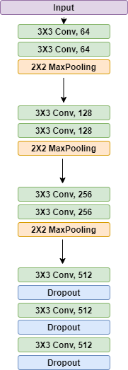
A modified version of VGG-16 [Simonyan2015] is used as the encoder, in which the dense layers and the last convolutional block were removed, leaving the current adaptation with 4 blocks. The first 3 blocks contain 2 convolutional layers, each block followed by a MaxPooling layer. The last block holds 3 convolutional layers, each layer followed by Dropout [Cicuttin2016]. The architecture is depicted in Fig. 2.
After comparing this configuration with others, i.e., Inception v_3, Xception and Inception ResNet v_2, we concluded that VGG-16 has given the best results so far, as seen in Section 4.2.3 . This allows the extraction of the input image features with high resolution, using these features as input to the FPM.
3.2 Feature Pooling Module
The Feature Pooling Module receives the features from the encoder in order to correlate them at different scales, making it easier for the decoder to reconstruct the input image.
Lim [Lim2019] proposed a Feature Pooling Module, in which the features from a 3 X 3 convolutional layer are concatenated with the Encoder features, resulting as input to a next convolutional layer with dilation rate of 4. The features from this layer are then concatenated with the Encoder features, hence used as input to a convolutional layer with dilation rate of 8. The process repeats itself to a convolutional layer with dilation rate of 8. The output of every layer is concatenated with a pooling layer, resulting in a 5 X 64 multi-features layers. These will finally be passed through InstanceNormalization and SpatialDropout.
After numerous experiments and tests, an improvement to this configuration was made. A convolutional layer with dilation rate of 2 is introduced, followed by the removal of the pooling layer. The output of the last layer, i.e., convolutional with dilation rate of 16, proceeds to BatchNormalization [Ioffe2015] (ensuring better results than InstanceNormalization) and SpatialDropout [Cicuttin2016] (Fig. 3).
Due to the removal of the multi-features layers, Dropout is used instead of SpatialDropout. The latter promoted independence between the resultant feature maps by dropping them in their entirety, correlating the adjacent pixels.

3.3 Training details
The proposed method receives a raw image and its corresponding mask, i.e., ground-truth, as input, both with 512 width and height. A pre-trained VGG-16 is being used. The first three layer blocks of the VGG-16 are being frozen in order to apply transfer learning to our model, since the feature extraction has been learned in a different context, the current objective is to learn the new layers and relate their features with the new problem.
The binary cross entropy loss is used, assigning more weight to the foreground in order to alleviate the imbalancement in the data, i.e., number of foreground pixels much higher than the background ones, and also taking in consideration when there are not any foreground pixels. The optimizer used is Adam [Kingma2015], proposing better results amongst other tested optimizers, i.e., RMSProp, Gradient Descent, AdaGrad [Duchi2012] and AdaDelta [Zeiler2012], and the batch size is 4.
A maximum number of 80 epochs is defined, stopping the training if the validation loss does not improve after 10 epochs, this can be achieved by using the early stopping callback.
The learning rate starts at 1e-4, and is reduced after 5 epochs by a factor of 0.1 if the learning stagnates, by applying a reduce on plateau callback.
4 Experiments and results
When the training is concluded, a test set containing the raw images and their corresponding masks is loaded, along with the trained model. For each loaded image a probability mask is produced by applying a specific threshold in order to remove the low probability scores. These probabilities are traduced in a Jet heatmap, i.e., when the color is red there is a high probability and when the color is purple there is a low probability of containing an anomaly, which will be blend with the corresponding raw image, making it easier to analyse the results. To complement these visual results, some metrics are also being applied.
4.1 Metrics
In order to fully understand the viability of the model, three different metrics are the focus throughout the evaluation.
The first one is the AUC ( Area Under Curve ) [Flach2011], it is equal to the probability that the classifier will rank a randomly chosen positive example higher than a randomly chosen negative example. This metrics allows the perception of the model detecting an object correctly, i.e., if the AUC is equal to 100% then the model detected every object in it. Nevertheless, this metric only focus on classification successes, failing to consider classification errors and not providing information regarding the segmentation.
The Accuracy and the F-Measure could be potential candidates, since they are highly used and usually produce reliable results, however, since the dataset is highly imbalanced when regarding the foreground and the background pixels, these two metrics are not an option, since they are highly sensitive to imbalanced data, therefore MCC (Mathews Correlation Coefficient ) is used as an alternative [Chicco2020]. This metric ranges from where represents a perfect segmentation according to the ground truth, and the opposite.
To complement the previous metric, the mIoU ( mean intersection over union ) is also used. IoU is the area of overlap between the predicted segmentation and the ground truth divided by the area of union between the predicted segmentation and the ground truth, and when applied to a binary classification, a mean is calculated by taking the IoU of each class and averaging them. This metric ranges from where represents a perfect overlap with the groundtruth and no overlap at all.
Nevertheless, metrics such as Recall, Specificity, PWC ( Percentage of wrong classifications ), Precision and F-Measure are also going to be used in some cases, in order to compare this proposed method with other state of the art.
4.1.1 Datasets
Three different datasets are used throughout the project. The first one is CityScapes, which pretends to capture images regarding outdoor street scenes [Ramos]. Every image was acquired with a camera in a moving vehicle across different months, this way different scenarios were covered, such as seasons and different cities. It has coarse pixel-level annotations, where of them were manually selected for dense pixel-level annotations. This way, there will be high diversity in foreground objects, background and scene layout. This dataset contains an additional challenge due to the moving camera.
The second is CDNet2014 dataset [Wang2014], it consists of 31 camera-captured videos with a fixed camera, containing eleven categories: Baseline, Dynamic Background, Camera Jitter, Intermittent Object Motion, Shadows, Thermal, Challenging Weather, Low Frame-Rate, Night, PTZ and Air Turbulence. The spatial resolution from the captured images ranges from 320x240 to 720x576. This dataset covers various challenging anomaly detections, both indoor and outdoor, making it useful to use in this proposed solution.
The last dataset is SBI2015 ( Scene Background Initialization ) [Christodoulidis2015]. It contains frames taken with a fixed camera from 14 video sequences with its corresponding ground-truths. It was assembled with the objective of evaluating and comparing the results of background initialization algorithms.
4.2 Experiments
Using [Lim2019] as a starting point, some ablation tests were made in order to understand the importance of the different components in the architecture and what could be improved. The metrics used throughout these evaluations are stated in 4.1, in order to compare each one from the previous analysis.
4.2.1 Feature Pooling Module
The first step was to break down the Feature Pooling Module, understanding the importance of it and if improvements could be done.
The first approach consists in changing the layers with different dilation rates, these dilated convolutions are used in order to systematically aggregate multi-scale
contextual information without losing resolution [Yu2016]. The tests are (1) Removing the convolutional layer with dilation rate equal to , (2) Add a convolutional layer with dilation rate equal to and (3) Add a convolutional layer with dilation rate equal to and remove a convolutional layer with dilation rate equal to .
As seen in Tab. 2, when removing the layer with dilation rate of , information is going to be lost, while when adding a layer with dilation rate equal to , there is going to be more obtained information from the images. Since the layer with dilation rate equal to improves the overall results, it will remain for the duration of the project.
| Baseline | LowFrameRate | BadWeather | CameraJitter | |||||||||
|---|---|---|---|---|---|---|---|---|---|---|---|---|
| F-M. | MCC | mIoU | F-M. | MCC | mIoU | F-M. | MCC | mIoU | F-M. | MCC | mIoU | |
| (1) | 0.9491 | 0.9313 | 0.9317 | 0,625 | 0.6870 | 0.6930 | 0.8916 | 0.8817 | 0.8927 | 0.9030 | 0.8912 | 0.9000 |
| (2) | 0.9731 | 0.9697 | 0.9721 | 0.7102 | 0.7054 | 0.7098 | 0.9172 | 0.9102 | 0.9148 | 0.9218 | 0.9199 | 0.9205 |
| (3) | 0.9528 | 0.9487 | 0.9510 | 0.6970 | 0.6890 | 0.6900 | 0.9034 | 0.8987 | 0.9019 | 0.9190 | 0.9076 | 0.9119 |
The second approach is to change some of the concatenations between the layers. These tests consist in (1) Remove output from layer with dilation rate of 2 to the final concatenations, (2) Only concatenate layer with dilation rate=16 to the pooling and layer with r=1, Figure 68, (3) Delete every connection from pooling layer, (4) Only keep the final output of layer with dilation rate of 16 as input to the SpatialDropout and (5) Delete every concatenation.
As seen in Tab. 2, when comparing the concatenations, (3) and (4) produce the best results. Hence, the other concatenation tests will be discarded, keeping these two in the next tests.
| Baseline | LowFrameRate | BadWeather | CameraJitter | |||||||||
|---|---|---|---|---|---|---|---|---|---|---|---|---|
| F-M. | MCC | mIoU | F-M. | MCC | mIoU | F-M. | MCC | mIoU | F-M. | MCC | mIoU | |
| (1) | 0.9281 | 0.9198 | 0.9260 | 0.6623 | 0.6596 | 0.6602 | 0.8916 | 0.8897 | 0.8904 | 0.9082 | 0.9047 | 0.9058 |
| (2) | 0.9528 | 0.9502 | 0.9516 | 0.6898 | 0.6885 | 0.6890 | 0.8994 | 0.8978 | 0.8983 | 0.9036 | 0.9011 | 0.9023 |
| (3) | 0.9804 | 0.9789 | 0.9799 | 0.7328 | 0.7311 | 0.7320 | 0.9207 | 0.9200 | 0.9202 | 0.9386 | 0.9368 | 0.9374 |
| (4) | 0.9824 | 0.9817 | 0.9820 | 0.7517 | 0.7502 | 0.7513 | 0.9305 | 0.9296 | 0.9300 | 0.9492 | 0.9486 | 0.9490 |
| (5) | 0.9528 | 0.9518 | 0.9520 | 0.6917 | 0.6909 | 0.6912 | 0.8923 | 0.8917 | 0.8920 | 0.9029 | 0.9010 | 0.9019 |
Three additional tests were made to the FPM. (1) Remove the input F from every layer, except the pooling layer and the layer with dilation rate of 1, (2) Remove the FPM, (3) Delete the pooling layer.
4.2.2 Decoder
The decoder in [Lim2019] uses three Convolutional layers 3X3, followed by InstanceNormalization, and multiplies the output of the first two layers with the output of the Encoder and GlobalAveragePooling (GAP).
The first step consists in analysing the importance of the GAP, maintaining the output of the Encoder or removing it ( according to its corresponding GAP ). The tests are (1) Remove the first GAP and its corresponding Encoder’s output, (2) Remove the second GAP and its corresponding Encoder’s output, (3) Remove both GAP and the Encoder’s output, (4) Remove first GAP but keep the corresponding Encoder’s output, (5) Remove second GAP but keep the corresponding Encoder’s output and (6) Remove both GAP but keep both Encoder’s output.
As seen in Tab. LABEL:tab:GAP1, (4) and (6) produce the worst results, decreasing the AUC, MCC and mIoU. As for the other configurations, they produce an overall increase in every metric, nevertheless when removing both GAP modules and the Encoder’s outputs, the MCC and mIoU record the highest values, therefore the other configurations will be discarded, keeping (3).
| Baseline | LowFrameRate | |||
|---|---|---|---|---|
| F-M. | MCC | F-M. | MCC | |
| (1) | 0.9527 | 0.9502 | 0.8010 | 0.7927 |
| (2) | 0.9683 | 0.9650 | 0.8438 | 0.8412 |
| (3) | 0.9856 | 0.9851 | 0.9680 | 0.9655 |
| (4) | 0.8716 | 0.8678 | 0.7617 | 0.7600 |
| (5) | 0.9628 | 0.9611 | 0.8017 | 0.8000 |
| (6) | 0.8847 | 0.8826 | 0.7729 | 0.7711 |
After analysing the GAP, the possible importance of the multiplications between the output of the first two layers in the Decoder and the output of the Encoder after applying the GAP must be considered, therefore additional tests regarding this topic were made. (1) Remove first multiplication, (2) Remove second multiplication and (3) Remove both multiplications.
As seen in LABEL:tab:GAP2 the results decrease when compared to removing both GAP, hence these configurations will be discarded.
| Baseline | LowFrameRate | |||
|---|---|---|---|---|
| F-M. | MCC | F-M. | MCC | |
| (1) | 0.8926 | 0.8911 | 0.8618 | 0.8601 |
| (2) | 0.9327 | 0.9316 | 0.9137 | 0.9122 |
| (3) | 0.9126 | 0.9111 | 0.9017 | 0.8985 |
4.2.3 Encoder
Keeping the previous configurations of the FPM and the Decoder, three tests were made in the Encoder, changing the VGG-16 backbone to (1) Inception v3 [Szegedy2016], (2) Xception [Chollet2017] and (3) Inception ResNet v2 [Szegedy2017].
When comparing these three with the VGG-16, the latter produces better results in every metric while also keeping the number of features much lower, as seen in Tab. 5.
| (1) | (2) | (3) | ||
|---|---|---|---|---|
| Baseline | F-M. | 0.8816 | 0.9014 | 0.9218 |
| MCC | 0.8798 | 0.9002 | 0.9202 | |
| mIoU | 0.8803 | 0.9010 | 0.9212 | |
| LowFr.R. | F-M. | 0.8126 | 0.8428 | 0.8828 |
| MCC | 0.8109 | 0.8406 | 0.8811 | |
| mIoU | 0.8111 | 0.8416 | 0.8820 |
4.3 Final results and Comparison
With the previous configurations established, some results applied to the full datasets are compared with the state of the art.
Regarding the CDNet2014 dataset, the proposed method outperforms the top state of the art technique in this dataset, i.e., FgSegNet_v2, when using 200 frames for training, improving by a long margin the LowFrameRate class, going from 0.8897 to 0.9939 in the F-Measure, more details in Tab. 6. Some visual results can also be seen in Fig. 4, presenting results close to the ground truth, even when dealing with LowFrameRate images.
| FPR | FNR | Recall | Precision | PWV | F-Measure | MCC | mIoU | ||
|---|---|---|---|---|---|---|---|---|---|
| Baseline | (1) | 6e-4 | 2e-3 | 0.9979 | 0.9974 | 0.0129 | 0.9975 | 0.9973 | 0.9975 |
| (2) | 4e-4 | 3.8e-3 | 0.9962 | 0.9985 | 0.0117 | 0.9936 | 0.9932 | 0.9933 | |
| Low Fr. | (1) | 4.8e-3 | 4.1e-3 | 0.9956 | 0.9910 | 0.0569 | 0.9939 | 0.9931 | 0.9934 |
| (2) | 8e-4 | 9.5e-2 | 0.9044 | 0.8782 | 0.0299 | 0.8897 | 0.8889 | 0.8893 | |
| Night V. | (1) | 7.4e-4 | 1.5e-2 | 0.9848 | 0.9785 | 0.1245 | 0.9816 | 0.9811 | 0.9814 |
| (2) | 2.2e-4 | 3.6e-2 | 0.9637 | 0.9861 | 0.0802 | 0.9747 | 0.9741 | 0.9745 | |
| PTZ | (1) | 6e-4 | 2.3e-2 | 0.9888 | 0.9902 | 0.0471 | 0.9922 | 0.9918 | 0.9920 |
| (2) | 4e-4 | 2.1e-2 | 0.9785 | 0.9834 | 0.0128 | 0.9809 | 0.9801 | 0.9803 | |
| Turbulence | (1) | 3e-4 | 2.5e-2 | 0.9861 | 0.9826 | 0.0417 | 0.9878 | 0.9867 | 0.9870 |
| (2) | 1.1e-4 | 2.2e-2 | 0.9779 | 0.9747 | 0.0232 | 0.9762 | 0.9722 | 0.9738 | |
| Bad Wea. | (1) | 1.3e-4 | 1e-2 | 0.9913 | 0.9914 | 0.0379 | 0.9881 | 0.9878 | 0.9880 |
| (2) | 9e-5 | 2.1e-2 | 0.9785 | 0.9911 | 0.0295 | 0.9848 | 0.9843 | 0.9845 | |
| Dyn.Back. | (1) | 3e-5 | 7.4e-3 | 0.9958 | 0.9959 | 0.0067 | 0.9960 | 0.9957 | 0.9959 |
| (2) | 1.5e-4 | 1e-2 | 0.9925 | 0.9840 | 0.0054 | 0.9881 | 0.9878 | 0.9880 | |
| Cam.Jitter | (1) | 1.6e-4 | 2.5e-3 | 0.9974 | 0.9940 | 0.0275 | 0.9957 | 0.9952 | 0.9955 |
| (2) | 1.2e-4 | 9.3e-3 | 0.9907 | 0.9965 | 0.0438 | 0.9936 | 0.9930 | 0.9933 | |
| Int.Obj.Mot. | (1) | 2.3e-4 | 7.4e-3 | 0.9925 | 0.9972 | 0.0672 | 0.9948 | 0.9945 | 0.9946 |
| (2) | 1.5e-4 | 1e-2 | 0.9896 | 0.9976 | 0.0707 | 0.9935 | 0.9932 | 0.9934 | |
| Shadow | (1) | 4e-4 | 1.6e-2 | 0.9909 | 0.9942 | 0.0542 | 0.9938 | 0.9935 | 0.9936 |
| (2) | 2.4e-4 | 8.9e-3 | 0.9911 | 0.9947 | 0.0575 | 0.9929 | 0.9919 | 0.9924 | |
| Thermal | (1) | 2e-4 | 2.7e-3 | 0.9972 | 0.9954 | 0.0302 | 0.9963 | 0.9959 | 0.9962 |
| (2) | 1e-4 | 5.6e-3 | 0.9944 | 0.9974 | 0.0290 | 0.9959 | 0.9951 | 0.9954 |

In the SBI2015 dataset, the overall F-Measure decreased from 0.9853 to 0.9447 when compared with the FgSegNet_v2, but increased from 0.8932 to 0.9447 when compared with the CascadeCNN, [Wang2017-2]. Nevertheless, the results still confirm a good overall evaluation on this dataset, compensating the higher results assembled in the CDNet2014 dataset. More details can be seen in Tab. LABEL:tab:sbi.
| AUC | F-M. | MCC | |
|---|---|---|---|
| Board | 99.84 | 0.9734 | 0.9724 |
| Candela | 99.92 | 0.9640 | 0.9631 |
| CAVIAR1 | 97.25 | 0.9475 | 0.9466 |
| CAVIAR2 | 97.51 | 0.9011 | 0.9001 |
| Cavignal | 99.94 | 0.9881 | 0.9872 |
| Foliage | 99.10 | 0.9124 | 0.9115 |
| HallAndMonitor | 98.49 | 0.9169 | 0.9160 |
| Highway1 | 99.35 | 0.9593 | 0.9583 |
| Highway2 | 99.56 | 0.9528 | 0.9518 |
| Humanbody2 | 99.82 | 0.9579 | 0.9580 |
| IBMtest2 | 99.42 | 0.9521 | 0.9512 |
| PeopleAndFoliage | 99.77 | 0.9570 | 0.9560 |
| Snellen | 98.84 | 0.8977 | 0.8967 |
Last, in the CityScapes dataset, a test was made in three different classes (Road, Citizens and Traffic Signs). As seen in Tab. LABEL:tab:cityscapes and in Fig. 5, the proposed method is able to detect almost every object, confirmed by the AUC, making a good segmentation on them.
| AUC | MCC | mIoU | |
|---|---|---|---|
| Road | 99.61 | 0.9555 | 0.9564 |
| Citizens | 99.31 | 0.7552 | 0.8019 |
| Traffic Signs | 97.72 | 0.6618 | 0.7425 |

5 CONCLUSION
An improved FgSegNet_v2 is proposed in the presented paper. By changing the Feature Pooling Module, i.e., deleting the pooling layer and only maintaining the output from the layer with dilation rate of 16, and the Decoder, i.e., removing the GAP modules, a more simplified and efficient approach is made, preserving the low number of needed training images feature while improving the overall results. Making some changes in the training configuration, e.g., batch size and optimizer, also improved the proposed method. It outperforms every state of the art method in the ChangeDetection2014 challenge, specially in the LowFrameRate images, showing a tremendous improvement and also maintaining great results in the SBI and CityScapes datasets, resulting in a more generalized method than the others since no experiments have been shown when using these datasets simultaneously. As future work, the proposed method is going to focus on the CityScapes dataset since more tests need to be done with different classes, maintaining or improving the good results in other datasets.