Anomalously Reduced Homogeneous Broadening of Two-Dimensional Electronic Spectroscopy at High Temperature by Detailed Balance

As known to all, multitransition and higher temperature can induce more significant decoherence and thus result in broader line width Mukamel (1999); Breuer and Petruccione (2002). However, it has been theoretically predicted and experimentally observed that the multitransition of a nitrogen-vacancy (NV) center in diamond can have longer coherence time than the single transitions, due to manipulation of the quantum bath evolution via flips of the center spin Zhao et al. (2011); Huang et al. (2011). Therefore, it might be interesting to investigate the effect of the temperature on the homogeneous broadening in spectroscopies. In this paper, we theoretically demonstrate that the homogeneous broadening of the two-dimensional electronic spectroscopy (2DES) in the presence of the electromagnetically-induced transparency (EIT) can be anomalously reduced at higher temperatures because of the detailed balance.

In recent years, two-dimensional electronic spectroscopy (2DES) has emerged as a powerful tool for investigating the ultrafast dynamics of complex quantum systems Mukamel (1999); Weng and Chen (2013); Cho (2008); Mukamel (2000); Chernyak and Mukamel (1995); Jonas (2003); Biswas et al. (2022); Hamm and Zanni (2011); Moody and Cundiff (2017); Fuller and Ogilvie (2015), including quantum wells Turner and Nelson (2010), quantum dots and 2D materials Liu et al. (2019); Moody et al. (2015), perovskites Liu et al. (2021), organic photovoltaic cells Song et al. (2014); Bakulin et al. (2016); Jones et al. (2020); De Sio et al. (2016), photosynthetic complexes (Brixner et al., 2005; Engel et al., 2007; Collini et al., 2010; Romero et al., 2007; Fuller et al., 2014; Tiwari et al., 2013; Cao et al., 2020; Song et al., 2021; Son et al., 2019), NV centers in diamond (Huxter et al., 2013), and chiral molecules Cai et al. (2022). The fundamental theoretical framework of 2DES involves the application of three coherent laser pulse trains to samples, generating third-order polarization signals. Through the analysis of the nonlinear signals, 2DES can unveil nuanced aspects of electronic coherence, energy transfer pathways, and correlations within a wide array of physical systems. Notably, explorations of ultrafast processes in molecular aggregates, photosynthetic complexes, and semiconductor nanostructures has unearthed fundamental principles governing the dynamics of excited states. Given that the time-correlation function intricately influences quantum dynamics in conjunction with the system Hamiltonian, the center-line slope of 2DES has been proposed as a means to extract information regarding system-bath interaction under various conditions (Kwak et al., 2007; Rosenfeld et al., 2011; Sun et al., 2023). When spectral line bands from different processes overlap, making it challenging to distinguish distinct peaks Roberts et al. (2006), the ability of 2DES to resolve both the structure and dynamics is significantly hindered. The problem tends to get worse as the environment around a molecule becomes more diverse. As a result, the application of 2DES is significantly limited by the spectral line width.

On the other hand, the EIT has been widely used to realize optical non-reciprocity Zhang et al. (2018); Huang et al. (2022), suppress dissipation in artificial light-harvesting systems Dong et al. (2012), and polarize the nuclear spin at the vicinity of NV centers in diamond Dutt et al. (2007); Wang et al. (2018a). Intuitively, it may be natural to utilize the EIT to effectively improve the signal-noise ratio of 2DES (Liu et al., 2020). The previous investigation proposes utilizing the quantum optical EIT effect to improve multi-dimensional spectroscopic measurements beyond the standard resolution limits Liu et al. (2020). However, at high temperature, only the downhill population relaxation has been taken into account, while the uphill population relaxation has been neglected therein. In other words, the whole relaxation does not fulfill the detailed-balance condition Mukamel (1999); Breuer and Petruccione (2002). But it is worth noting that under non-zero temperature conditions, the uphill population relaxation in combination with the downhill population relaxation drive the open quantum system towards the steady state described by the Boltzmann distribution Mukamel (1999); Breuer and Petruccione (2002). It is this fundamental principal that inspires us to take into account this overlooked crucial information and consider the influence of temperature on the spectral resolution, making it more aligned with real-world scenarios.

The rest of the paper is structured as follows. In Sec. II, we introduce the theoretical model and perform calculations based on the response functions. In Sec. III, numerical simulation results are presented and analyzed. Sec. IV describes the physical implementation. Finally, a summary and discussion are provided in Sec. V. In Appendixes A and B, we derive the master equations for a two-level system and a four-level system, respectively. In Appendix C, we discuss the whole rephasing signal.

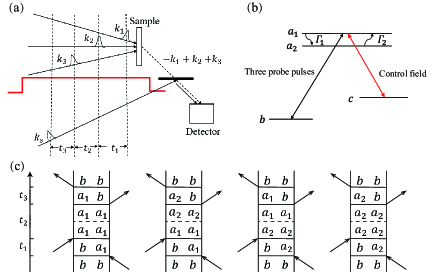
In essence, the two-dimensional spectroscopy is the third-order nonlinear polarization signal generated by the interaction of three coherent ultra-short laser pulses with the substance Mukamel (1999), where the heterodyne detection method is applied to detect the signal. As shown in Fig. 1(b), four pulses are applied, including three short probe pulses and one long control field. The first probe pulse is temporally centered at $t=0$, and the next two probe pulses are delayed by $t_{1}$ and $t_{2}$ in time successively. Finally, a heterodyne pulse is applied after the time interval $t_{3}$. The first three ultra-short laser pulses generate a signal, which is heterodyne detected by a fourth pulse in a specific phase-matching direction. In 2DES, excitation frequency axis $\omega_{1}$ and detection frequency axis $\omega_{3}$ are the Fourier transform of the time delays $t_{1}$ and $t_{3}$, respectively. In addition to a sequence of four pulses commonly-used in traditional two-dimensional spectroscopy, a narrow-band control field is applied to drive a specific transition between the energy levels $a_{1}$ and $c$ in Fig. 1(b). Here, broadband probe pulses can drive the transitions between $b$ and $a_{j}$ $(j=1,2)$.

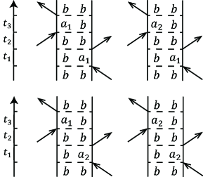
Without loss of generality, we first consider the 2DES generated by the $R_{2}$ path, that is, the stimulated emission process in the direction of $k_{s}=-k_{1}+k_{2}+k_{3}$. Here, four Feynman diagrams can be drawn for the $R_{2}$ path, as shown in Fig. 1(c). We remark that in the three-level case, i.e., $a_{2}$ is absent, there is only one kind of Feynman diagram for the $R_{2}$ path, which is not shown here. And the broadband probe pulses can not induce the transitions $a_{1}\rightleftharpoons a_{2}$ and $c\rightleftharpoons a_{j}$, but $b\rightleftharpoons a_{j}$ $(j=1,2)$.

The total Hamiltonian including the interaction between the system and the control field reads

where $\omega_{j}$ is the energy of the state $|j\rangle$ $(j=b,a_{1},a_{2},c)$, we assume $\hbar=1$ for simplicity, $\Omega=\mu_{a_{1}c}\varepsilon_{c}$ is the Rabi frequency with $\mu_{a_{1}c}$ being the transition dipole moment, $\varepsilon_{c}$ and $\nu_{c}$ being the amplitude and the frequency of the control field, respectively. Here, $\omega_{a_{2}}$ is adjustable in our investigation.

Generally, the quantum dynamics are governed by the quantum master equation $\dot{\rho}=-\frac{i}{\hbar}[H,\rho]-\varGamma_{1}\mathcal{L}(A_{a_{2}a_{1}})\rho-\varGamma_{2}\mathcal{L}(A_{a_{1}a_{2}})\rho$ (Olaya-Castro et al., 2008; Mukamel, 1999; Dong et al., 2012), where $\mathcal{L}(A_{\alpha\beta})\rho=\frac{1}{2}\{A^{\dagger}_{\alpha\beta}A_{\alpha\beta},\rho\}-A_{\alpha\beta}\rho A^{\dagger}_{\alpha\beta}$ with $\{A^{\dagger}_{\alpha\beta}A_{\alpha\beta},\rho\}$ being the anti-commutator, $A_{\alpha\beta}=|\alpha\rangle\langle\beta|$ is the quantum jump operator from the initial state $|\beta\rangle$ to the final state $|\alpha\rangle$. The exact quantum dynamics can be obtained by the hierarchical equation of motion, which can be exponentially accelerated by a recently-developed quantum algorithm Wang et al. (2018b); Zhang et al. (2021). However, under certain circumstances, the quantum master equation approach without the quantum-jump term can provide an analytical result and thus effectively help us grasp the underlying mechanism. In the interaction picture, assuming $\nu_{c}=\omega_{a_{1}}-\omega_{c}$, the time evolution of the density matrix is determined by

where $\gamma_{a_{1}c}=(\varGamma_{1}+\varGamma_{c})/2+\gamma^{(0)}_{a_{1}c}$, the population relaxation rates between the states $a_{1}$ and $a_{2}$ are respectively $\varGamma_{1}$ and $\varGamma_{2}$, between which the relation is governed by the detailed balance (Breuer and Petruccione, 2002). $\gamma^{(0)}_{a_{1}c}$ is the pure-dephasing rate between states $a_{1}$ and $c$. Here, we have assumed that the population relaxation $\varGamma_{c}$ of the metastable state $c$ can be neglected. As a result, we can obtain the Green function as

where $\widetilde{\Omega}=\sqrt{4\Omega^{2}-\gamma_{a_{1}c}^{2}}$, $A_{1}=\varGamma_{1}+\varGamma_{2}$, $A_{2}^{\pm}=[\varGamma_{2}(\varGamma_{1}+\varGamma_{2}-\gamma_{a_{1}c})+\Omega^{2}](i\widetilde{\Omega}\pm\gamma_{a_{1}c})\mp 2\varGamma_{1}\Omega^{2}$, $A_{3}=-(\varGamma_{1}+\varGamma_{2})(\varGamma_{1}+\varGamma_{2}-\gamma_{a_{1}c})-\Omega^{2}$, $A_{4}=2A_{3}+\Omega^{2}$, $B_{1}=-2(\varGamma_{1}+\varGamma_{2})(\varGamma_{1}+\varGamma_{2}-\gamma_{a_{1}c})-\Omega^{2}$, $B_{2}=(B_{1}-\Omega^{2})/2$, $B_{3}=(\varGamma_{1}+\varGamma_{2}-\gamma_{a_{1}c})(\gamma_{a_{1}c}+i\widetilde{\Omega})+2\Omega^{2}$ and $B_{4}=(\varGamma_{1}+\varGamma_{2}-\gamma_{a_{1}c})(-\gamma_{a_{1}c}+i\widetilde{\Omega})-2\Omega^{2}$.

If we consider the $R_{2}$ term in the rephrasing case, the response function is written as Mukamel (1999)

where $\mu_{ba_{i}}$ is the transition dipole moment between the states $b$ and $a_{i}$ ($i=1,2$).

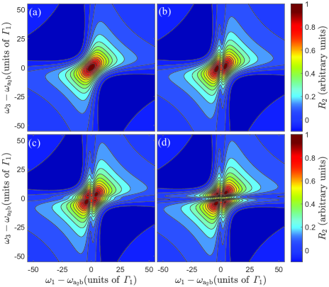
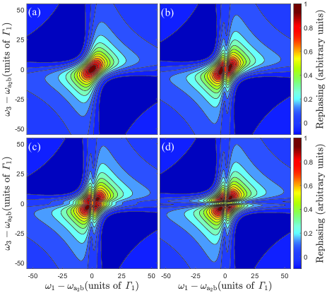
We investigate the effect of temperature on the 2DES under the near-resonant condition in the long-population-time limit, as shown in Fig. 2. When there is no control field, there is only one peak in Fig. 2(a) due to the absence of EIT. If the control field is applied, e.g. Fig. 2(b), the diagonal peak is split into two peaks, in which the homogeneous broadening is partially reduced. However, if the temperature is increased, e.g. $k_{B}T=0.1\varGamma_{1}$ in Fig. 2(c), two additional small peaks begin to emerge at the side of the above two peaks. Interestingly, if temperature is sufficiently high, i.e., $k_{B}T=5\varGamma_{1}$ in Fig. 2(d), the original large peak in Fig. 2(a) is almost evenly split into four peaks. Notice that the homogeneous broadening is even narrower than that in Fig. 2(b), which has been significantly reduced due to the EIT. In general, the downhill and uphill rates fulfill the detailed balance (Breuer and Petruccione, 2002). At the absolute zero temperature, there is only population transfer from the higher level to the lower one. As the temperature increases, the population-back transfer emerges due to the heating by the bath. We remark that the combination of the heating and the EIT results in the eliminating of homogeneous broadening in the long-population-time limit.

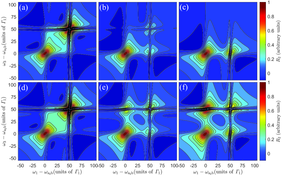
In order to illustrate the underlying physical mechanism explicitly, we consider the case of a large detuning between the two levels $a_{1}$ and $a_{2}$. We discuss the $k_{B}T=\varGamma_{1}$ case as shown in the upper panel of Fig. 3, i.e., at low temperatures. When $t_{2}=0$, there are two sets of diagonal peaks at $\omega_{a_{j}b}$ ($j=1,2$), respectively. The diagonal peak at $\omega_{a_{1}b}$ is split into four small peaks due to the EIT introduced by the control field, which induces the transition between $a_{1}$ and $c$, while the diagonal peak at $\omega_{a_{2}b}$ remains as a whole large peak. When the population time elapses, e.g. $t_{2}=0.5\varGamma_{1}^{-1}$, a set of off-diagonal peaks at ($\omega_{a_{1}b},\omega_{a_{2}b}$) emerge due to the population transfer from level $a_{1}$ to $a_{2}$. And generated by the processes corresponding to the four Feynman diagrams in Fig. 1(c), the peaks in 2DES which overlap with each other in the nearly-resonant case will be separated. When the population time is sufficiently long, e.g. $t_{2}=5\varGamma_{1}^{-1}$, we can observe from the spectroscopy that the peaks at $\omega_{3}=\omega_{a_{1}b}$ have disappeared and the peak in the bottom right corner has been enhanced. And that’s because in the long-population-time limit, i.e., $t_{2}\gg\varGamma_{1}^{-1}$, the entire population of the level $a_{1}$ has been unidirectionally transferred to the level $a_{2}$. The lower panel of Fig. 3 is simulated at $k_{B}T=10^{3}\varGamma_{1}$, that is, at a sufficiently-high temperature. In the case of $t_{2}=0$, we can not discriminate the difference between Fig. 3(d) for $k_{B}T=10^{3}\varGamma_{1}$ and Fig. 3(a) for $k_{B}T=\varGamma_{1}$. When $t_{2}=0.5\varGamma_{1}^{-1}$, two off-diagonal peaks appear in Fig. 3(e). In addition to the one in Fig. 3(b), there is one at ($\omega_{a_{2}b},\omega_{a_{1}b}$) because of the population-back transfer from the lower level to the higher level due to heating by the bath. At $t_{2}=5\varGamma_{1}^{-1}$, the peaks in these four regions of Fig. 3(f) do not disappear, which is quite different from the observation in the case of $k_{B}T=\varGamma_{1}$. Because of non-vanishing $\varGamma_{2}$, the bidirectional population transfer between levels $a_{1}$ and $a_{2}$ always exists dynamically.

In a real system, there is not only the downhill relaxation from $a_{1}$ to $a_{2}$, but also the uphill relaxation from $a_{2}$ to $a_{1}$. The ratio of the two relaxation rates is determined by the temperature and the energy gap between $a_{1}$ and $a_{2}$. In order to observe the different scenarios as shown in Figs. 2-3, we can effectively adjust the energy gap between $a_{1}$ and $a_{2}$. As the energy gap increases, the 2DES obtained when $a_{1}$ and $a_{2}$ are nearly-resonant will split, and thus more detailed information about the dynamics under investigation will be revealed.

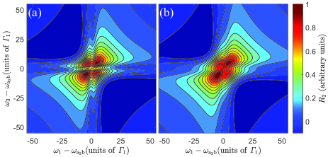
The average of inhomogeneous broadening will superpose 2DES with different level spacings $\omega_{a_{1}a_{2}}$ between $|a_{1}\rangle$ and $|a_{2}\rangle$. When the static disorder is small, the average of inhomogeneous broadening will not essentially modify our main findings, as shown in Fig. 4(a). As the static disorder increases, the homogeneous broadening will be enlarged due to the average of inhomogeneous broadening, as shown in Fig. 4(b). Therefore, we may safely arrive at the conclusion that the anomalously-reduced homogeneous broadening can be still observed as long as $\sigma<2.6\varGamma_{1}$, which is within the experimental observation $\sigma=1.4\varGamma_{1}$ Novoderezhkin et al. (2011a).

So far as the average of the interaction between the electric field and the transition dipole moments of molecules is considered, it will superpose 2DES with different widths of the gaps between the peaks in Fig. 2(d). If the electric field is big enough or the interaction between the electric field and the transition dipole moments of molecules are nearly identical, our main findings will not be essentially modified. In order to make the interaction between the electric field and the transition dipole moments of molecules nearly identical, we can initially prepare the sample to be crystal Zhao et al. (2023).

To demonstrate our theoretical proposal, we use the energy-level structure of two pheophytins, i.e., PheD1 and PheD2, in the PSII-RC. Their energies are respectively $E_{1}=15030~{}\mathrm{cm^{-1}}$ and $E_{2}=15020~{}\mathrm{cm^{-1}}$. The electronic coupling between them is $J=-3~{}\mathrm{cm^{-1}}$ Novoderezhkin et al. (2011b). We calculate the new energy levels of the dimer due to the coupling as $\varepsilon_{1}=(E_{1}+E_{2}+\Delta E)/2=15031~{}\mathrm{cm^{-1}}$ and $\varepsilon_{2}=(E_{1}+E_{2}-\Delta E)/2=15019~{}\mathrm{cm^{-1}}$ where $\Delta E=\sqrt{(E_{1}-E_{2})^{2}+4J^{2}}$ is the gap between two levels $a_{1}$ and $a_{2}$. In order to realize the four-level configuration in Fig. 1, we utilize a vibronic mode with frequency $745~{}\textrm{cm}^{-1}$ with relaxation rate $\varGamma_{b}=0.1~{}\mathrm{ps}^{-1}$ Reimers et al. (2013), i.e., $|b\rangle=|g\rangle|1\rangle_{v}$, $|c\rangle=|g\rangle|0\rangle_{v}$, $|a_{1}\rangle=|\varepsilon_{1}\rangle|0\rangle_{v}$, and $|a_{2}\rangle=|\varepsilon_{2}\rangle|0\rangle_{v}$, where $|0\rangle_{v}$ and $|1\rangle_{v}$ are respectively the ground and first excited state of the vibronic mode. The pure-dephasing rates are respectively $\gamma_{a_{1}c}^{(0)}=\gamma_{a_{1}b}^{(0)}=\gamma_{a_{2}b}^{(0)}=10\varGamma_{1}$ and $\gamma_{bc}^{(0)}=10\varGamma_{b}$. The Rabi frequency of the control field is $\Omega=9\varGamma_{1}$. The downhill population transfer rate is $\varGamma_{1}=10~{}\mathrm{ps}^{-1}$. Here, the uphill population transfer rate $\varGamma_{2}$ and $\varGamma_{1}$ satisfy the detailed-balance relation, i.e., $\varGamma_{2}/\varGamma_{1}=\textrm{exp}(-\Delta E/k_{B}T)$, where $T$ is the ambient temperature.

The proposed anomalous effect can be observed for a wide range of parameters, which will be elucidated as follows. First of all, the temperature must be sufficiently high to satisfy $\varGamma_{1}/\varGamma_{2}\approx 1$, which is easily achieved for a molecule with small level spacing, i.e., $\hbar\omega_{a_{1}a_{2}}\ll k_{B}T$. This is because the contributions from the off-diagonal peaks become more significant at higher temperatures. Secondly, the population time $t_{2}$ must exceed the inverse of the relaxation rate $1/\varGamma_{1}$, i.e., $t_{2}\varGamma_{1}>1$, ensuring that the off-diagonal peaks remain relatively stable over time. The last but not the least, the Rabi frequency of the control field needs to be sufficiently large, as the separation of the sub-peaks introduced by the EIT is proportional to the Rabi frequency. In this study, a significant phenomenon can be observed at $\Omega=9\varGamma_{1}$.

In this paper, we theoretically explore the anomalous reduction of homogeneous broadening in 2DES at high temperatures, which is attributed to the detailed balance assisted by the EIT. Compared with lower temperatures, the homogeneous broadening is much narrower at higher temperatures due to the long-lasting off-diagonal peaks, which vanish at the former case. Since in realistic experiments, $R_{2}$ can not be separated from the rephasing signal which also contains $R_{3}$, our discovery still holds when $R_{3}$ is included. When the static disorder is considered, the homogeneous broadening is remarkably suppressed as long as $\sigma<2.6\varGamma_{1}$, which is within the experimental observation.

We thank stimulating discussions with W.-T. He and N.-N. Zhang. This work is supported by Innovation Program for Quantum Science and Technology under Grant No. 2023ZD0300200, Beijing Natural Science Foundation under Grant No. 1202017 and the National Natural Science Foundation of China under Grant Nos. 62105030, 11674033, 11505007, and Beijing Normal University under Grant No. 2022129.

References

- Mukamel (1999) S. Mukamel, Principles of Nonlinear Optics and Spectroscopy (Oxford University Press, New York, 1999).
- Breuer and Petruccione (2002) H. P. Breuer and F. Petruccione, The Theory of Open Quantum Systems (Oxford University Presss, 2002).
- Zhao et al. (2011) N. Zhao, Z.-Y. Wang, and R.-B. Liu, “Anomalous decoherence effect in a quantum bath,” Phys. Rev. Lett. 106, 217205 (2011).
- Huang et al. (2011) P. Huang, X. Kong, N. Zhao, F. Shi, P. Wang, X. Rong, R. B. Liu, and J. Du, “Observation of anomalous decoherence effect in a quantum bath at room temperature,” Nat. Commun. 2, 570 (2011).
- Weng and Chen (2013) Y. X. Weng and H. L. Chen, Ultrafast Spectroscopy Principles and Techniques (Chemical Industry Press, Beijing, 2013).
- Cho (2008) M. Cho, “Coherent two-dimensional optical spectroscopy,” Chem. Rev. 108, 1331 (2008).
- Mukamel (2000) S. Mukamel, “Multidimensional femtosecond correlation spectroscopies of electronic and vibrational excitations,” Annu. Rev. Phys. Chem. 51, 691 (2000).
- Chernyak and Mukamel (1995) V. Chernyak and S. Mukamel, “Two-exciton collective photon echoes in disordered molecular nanostructures,” Phys. Rev. Lett. 74, 4895 (1995).
- Jonas (2003) D. M. Jonas, “Two-dimensional femtosecond spectroscopy,” Annu. Rev. Phys. Chem. 54, 425 (2003).
- Biswas et al. (2022) S. Biswas, J.-W. Kim, X.-Z. Zhang, and G. D. Scholes, “Coherent two-dimensional and broadband electronic spectroscopies,” Chem. Rev. 122, 4257 (2022).
- Hamm and Zanni (2011) P. Hamm and M. Zanni, Concepts and Methods of 2D Infrared Spectroscopy (Cambridge University Press, 2011).
- Moody and Cundiff (2017) G. Moody and S. T. Cundiff, “Advances in multi-dimensional coherent spectroscopy of semiconductor nanostructures,” Adv. Phys.: X 2, 641 (2017).
- Fuller and Ogilvie (2015) F. D. Fuller and J. P. Ogilvie, “Experimental implementations of two-dimensional fourier transform electronic spectroscopy,” Annu. Rev. Phys. Chem. 66, 667 (2015).
- Turner and Nelson (2010) D. B. Turner and K. A. Nelson, “Coherent measurements of high-order electronic correlations in quantum wells,” Nature 466, 1089 (2010).
- Liu et al. (2019) A. Liu, D. B. Almeida, W. K. Bae, L. A. Padilha, and S. T. Cundiff, “Non-Markovian exciton-phonon interactions in core-shell colloidal quantum dots at femtosecond timescales,” Phys. Rev. Lett. 123, 057403 (2019).
- Moody et al. (2015) G. Moody, C. K. Dass, K. Hao, C.-H. Chen, L.-J. Li, A. Singh, K. Tran, G. Clark, X.-D. Xu, G. Berghäuser, E. Malic, A. Knorr, and X.-Q. Li, “Intrinsic homogeneous linewidth and broadening mechanisms of excitons in monolayer transition metal dichalcogenides,” Nat. Commun. 6, 8315 (2015).
- Liu et al. (2021) A. Liu, D. B. Almeida, L. G. Bonato, G. Nagamine, L. F. Zagonel, A. F. Nogueira, L. A. Padilha, and S. T. Cundiff, “Multidimensional coherent spectroscopy reveals triplet state coherences in cesium lead-halide perovskite nanocrystals,” Sci. Adv. 7, eabb3594 (2021).
- Song et al. (2014) Y. Song, S. N. Clafton, R. D. Pensack, T. W. Kee, and G. D. Scholes, “Vibrational coherence probes the mechanism of ultrafast electron transfer in polymer-fullerene blends,” Nat. Commun. 5, 4933 (2014).
- Bakulin et al. (2016) A. A. Bakulin, S. E. Morgan, T. B. Kehoe, M. W. B. Wilson, A. W. Chin, D. Zigmantas, D. Egorova, and A. Rao, “Real-time observation of multiexcitonic states in ultrafast singlet fission using coherent 2D electronic spectroscopy,” Nat. Chem. 8, 16 (2016).
- Jones et al. (2020) A. C. Jones, N. M. Kearns, J.-J. Ho, J. T. Flach, and M. T. Zanni, “Impact of non-equilibrium molecular packings on singlet fission in microcrystals observed using 2D white-light microscopy,” Nat. Chem. 12, 40 (2020).
- De Sio et al. (2016) A. De Sio, F. Troiani, M. Maiuri, J. Réhault, E. Sommer, J. Lim, S. F. Huelga, M. B Plenio, C. A. Rozzi, G. Cerullo, E. Molinari, and C. Lienau, “Tracking the coherent generation of polaron pairs in conjugated polymers,” Nat. Commun. 7, 13742 (2016).
- Brixner et al. (2005) T. Brixner, J. Stenger, H. Vaswani, M. Cho, R. Blankenship, and G. Fleming, “Two-dimensional spectroscopy of electronic couplings in photosynthesis,” Nature 434, 625 (2005).
- Engel et al. (2007) G. S. Engel, T. R. Calhoun, E. L. Read, T.-K. Ahn, T. Mančal, Y.-C. Cheng, R. E. Blankenship, and G. R. Fleming, “Evidence for wavelike energy transfer through quantum coherence in photosynthetic systems,” Nature 446, 782 (2007).
- Collini et al. (2010) E. Collini, C. Y. Wong, K. E. Wilk, P. M. G. Curmi, P. Brumer, and G. D. Scholes, “Coherently wired light-harvesting in photosynthetic marine algae at ambient temperature,” Nature 463, 644 (2010).
- Romero et al. (2007) E. Romero, R. Augulis, V. I. Novoderezhkin, M. Ferretti, J. Thieme, D. Zigmantas, and R. van Grondelle, “Quantum coherence in photosynthesis for efficient solar-energy conversion,” Nat. Phys. 10, 676 (2007).
- Fuller et al. (2014) F. D. Fuller, J. Pan, A. Gelzinis, V. Butkus, S. S. Senlik, D. E. Wilcox, C. F. Yocum, L. Valkunas, D. Abramavicius, and J. P. Ogilvie, “Vibronic coherence in oxygenic photosynthesis,” Nat. Chem. 6, 706 (2014).
- Tiwari et al. (2013) V. Tiwari, W. K. Peters, and D. M. Jonas, “Electronic resonance with anticorrelated pigment vibrations drives photosynthetic energy transfer outside the adiabatic framework,” Proc. Natl. Acad. Sci. USA 110, 1203 (2013).
- Cao et al. (2020) J. Cao, R. J. Cogdell, D. F. Coker, H.-G. Duan, J. Hauer, U. Kleinekathöfer, T. L. C. Jansen, T. Mančal, R. J. Dwayne Miller, J. P. Ogilvie, V. I. Prokhorenko, T. Renger, H.-S. Tan, R. Tempelaar, M. Thorwart, E. Thyrhaug, S. Westenhoff, and D. Zigmantas, “Quantum biology revisited,” Sci. Adv. 6, eaaz4888 (2020).
- Song et al. (2021) Y. Song, R. Sechrist, H. H. Nguyen, W. Johnson, and J. P. Ogilvie, “Excitonic structure and charge separation in the heliobacterial reaction center probed by multispectral multidimensional spectroscopy,” Nat. Commun. 12, 2801 (2021).
- Son et al. (2019) M.-J. Son, A. Pinnola, R. Bassi, and G. S. Schlau-Cohen, “The electronic structure of lutein 2 is optimized for light harvesting in plants,” Chem 5, 575 (2019).
- Huxter et al. (2013) V. M. Huxter, T. Oliver, D. Budker, and G. R. Fleming, “Vibrational and electronic dynamics of nitrogen-vacancy centres in diamond revealed by two-dimensional ultrafast spectroscopy,” Nat. Phys. 9, 744 (2013).
- Cai et al. (2022) M.-R. Cai, C. Ye, H. Dong, and Y. Li, “Enantiodetection of chiral molecules via two-dimensional spectroscopy,” Phys. Rev. Lett. 129, 103201 (2022).
- Kwak et al. (2007) K. Kwak, S. Park, I. J. Finkelstein, and M. D. Fayer, “Frequency-frequency correlation functions and apodization in two-dimensional infrared vibrational echo spectroscopy: A new approach,” J. Chem. Phys. 127, 124503 (2007).
- Rosenfeld et al. (2011) D. E. Rosenfeld, Z. Gengeliczki, B. J. Smith, T. D. P. Stack, and M. D. Fayer, “Structural dynamics of a catalytic monolayer probed by ultrafast 2D IR vibrational echoes,” Science 334, 634 (2011).
- Sun et al. (2023) Z.-H. Sun, Y.-X. Yao, Q. Ai, and Y.-C. Cheng, “Theory of center-line slope in 2D electronic spectroscopy with static disorder,” Adv. Quantum Tech. 6, 2300163 (2023).
- Roberts et al. (2006) S. T. Roberts, J. J. Loparo, and A. Tokmakoff, “Characterization of spectral diffusion from two-dimensional line shapes,” J. Chem. Phys. 125, 084502 (2006).
- Zhang et al. (2018) S.-C. Zhang, Y.-Q. Hu, G.-W. Lin, Y.-Q. Niu, K.-Y. Xia, J.-B. Gong, and S.-Q. Gong, “Thermal-motion-induced non-reciprocal quantum optical system,” Nat. Photon. 12, 744 (2018).
- Huang et al. (2022) H.-B. Huang, J.-J. Lin, Y.-X. Yao, K.-Y. Xia, Z.-Qi Yin, and Q. Ai, “Optical nonreciprocity in rotating diamond with nitrogen-vacancy color centers,” Ann. Phys. (Berlin) 534, 2200157 (2022).
- Dong et al. (2012) H. Dong, D.-Z. Xu, J.-F. Huang, and C.-P. Sun, “Coherent excitation transfer via the dark-state channel in a bionic system,” Light Sci. & Appl. 1, e2 (2012).
- Dutt et al. (2007) M. V. Gurudev Dutt, L. Childress, L. Jiang, E. Togan, J. Maze, F. Jelezko, A. S. Zibrov, P. R. Hemmer, and M. D. Lukin, “Quantum register based on individual electronic and nuclear spin qubits in diamond,” Science 316, 1312 (2007).
- Wang et al. (2018a) Y.-Y. Wang, J. Qiu, Y.-Qi Chu, M. Zhang, J.-M. Cai, Q. Ai, and F.-G. Deng, “Dark state polarizing a nuclear spin in the vicinity of a nitrogen-vacancy center,” Phys. Rev. A 97, 042313 (2018a).
- Liu et al. (2020) G. Liu, A. S. Sizhuk, and K. E. Dorfman, “Selective elimination of homogeneous broadening by multidimensional spectroscopy in the electromagnetically induced transparency regime,” J. Phys. Chem. Lett. 11, 5504 (2020).
- Olaya-Castro et al. (2008) A. Olaya-Castro, C. F. Lee, F. F. Olsen, and N. F. Johnson, “Efficiency of energy transfer in a light-harvesting system under quantum coherence,” Phys. Rev. B 78, 085115 (2008).
- Wang et al. (2018b) B.-X. Wang, M.-J. Tao, Q. Ai, T. Xin, N. Lambert, D. Ruan, Y.-C. Cheng, F. Nori, F.-G. Deng, and G.-L. Long, “Efficient quantum simulation of photosynthetic light harvesting,” npj Quantum Inf. 4, 52 (2018b).
- Zhang et al. (2021) N.-N. Zhang, M.-J. Tao, W.-T. He, X.-Y. Chen, X.-Y. Kong, F.-G. Deng, N. Lambert, and Q. Ai, “Efficient quantum simulation of open quantum dynamics at various Hamiltonians and spectral densities,” Front. Phys. 16, 51501 (2021).
- Novoderezhkin et al. (2011a) V. I. Novoderezhkin, E. Romero, J. P. Dekker, and R. van Grondelle, “Multiple charge-separation pathways in photosystem II: Modeling of transient absorption kinetics,” ChemPhysChem 12, 681 (2011a).
- Zhao et al. (2023) X. T. Zhao, H. T. Zhang, J. Zhang, J. Liu, M. Lei, and L. Jiang, “Organic semiconductor single crystal arrays: Preparation and applications,” Adv. Sci. 10, 2300483 (2023).
- Novoderezhkin et al. (2011b) V. I. Novoderezhkin, E. Romero, J. P. Dekker, and R. van Grondelle, “Multiple charge-separation pathways in photosystem II: Modeling of transient absorption kinetics,” ChemPhysChem 12, 681 (2011b).
- Reimers et al. (2013) J. R. Reimers, Z.-L. Cai, R. Kobayashi, M. Rätsep, A. Freiberg, and E. Krausz, “Assignment of the Q-bands of the chlorophylls: Coherence loss via Qx-Qy mixing,” Sci. Rep. 3, 2761 (2013).
- Carmichael (1993) H. J. Carmichael, An Open Systems Approach to Quantum Optics (Spring-Verlag, Gemany, 1993).